Parsec and sub-parsec-scale structure and evolution in nearby compact radio sources and relationships to emission at other wavelengths

(1)

Parsec and Sub-Parsec-Scale Structure

and E volution in N earby Com pact Radio

Sources and R elationships to Em ission

at O ther W avelengths

Steven J. T ingay

A thesis submitted for the degree of

D o cto r o f P hilosophy

o f T he A ustralian N ational U niversity

Mount Stromlo and Siding Spring Observatories The Institute of Advanced Studies

The Australian National University Canberra, Australia

(2)

1

D isclaim er

I hereby declare that the work in this thesis is that of the candidate alone, except where indicated below. The co-authors of resulting papers contributed to the text of those papers.

C h a p te rs 3, 4, 5, 6, 7, a n d 8: The Southern Hemisphere VLBI Experiment team contributed to the observations of radio sources described in these chapters. C h a p te r 3: The VLBI data from 1991 March 13 were correlated and calibrated by D.W. Hoard (JPL) and J.E. Reynolds (ATNF).

C h a p te r 4: The VLBI data for PKS 0208-512, PKS 0438-436, PKS 0521-365, PKS 0537—441, and PKS 0637—752 were correlated partly bv T.D. van Ommen (JPL).

C h a p te r 5: Correlation of VLBI data from 1991 March 6, 1991 November 24, 1992 March 26, and 1992 November 22 was undertaken by T.D. van Ommen, M, St. John, and D.W. Hoard (JPL). Fringe-fitting of VLBI data from 1991 March 6, 1991 November 24 and 1992 March 26 was undertaken by D.W. Hoard, M. St. John, and D.L. Meier (JPL). Calibration of VLBI data from 1991 March 6 and 1991 November 24 was undertaken by J.E. Reynolds (ATNF).

C h a p te r 6: The calibration files for the VLBI observations were prepared by J.E. Reynolds. Part of the correlation of the VLBI data was undertaken by A.K. Tzioumis (ATNF).

C h a p te r 7: The 22 GHz Tidbinbilla observations were conducted by E.A. King (ATNF) and P. Harbison (British Aerospace Australia). The ATCA imaging ob servations were supervised by A. Koekemoer (MSSSO).

(3)

A cknow ledgem ents

At the completion of this work I take great pleasure in thanking and acknowledging the people who have supported me over the eight years of my university education, and in particular the last four years.

I could not have started down this path without the support and understanding of my family and my wife. Their encouragement has enabled me to pursue my goals with vigour. I hope that they can take as much pleasure from this finished work as I do.

I thank my PhD thesis supervisor, Dr David L. Jauncey of the Australia Tele scope National Facility. His guidance and insight has helped shape this work into what it is, and his careful proof reading of draft papers and the final the sis manuscript was very much appreciated. I am also grateful for the input of my advisor, Dr Geoffrey V. Bicknell of the Mount Stromlo and Siding Spring Obser vatories

I would like to thank the members of the Astronomical Measurements Group at the Jet Propulsion Laboratory in Pasadena, led by Dr Robert A. Preston. A substantial fraction of my time over the last 4 years has been spent at JPL, working in the AMG, without a doubt providing the most productive and enjoyable periods of my thesis.

Many other people have been involved in the work presented here, without whom the final results could not have been achieved. I refer here to the numerous people who have staffed the SHEVE telescopes over the last four years, changing tapes, making equipment work, and dealing with the logistics of getting an ad hoc

VLBI array up and running a few times per year with a great deal of success. These people are too many to thank individually but Dr John E. Reynolds and Dr Anastasios K. Tzioumis deserve special mention; they are the driving force behind much of what happens in the SHEVE operation.

Finally, this work was supported financially by an Australian Postgraduate Award. Financial support for travel was provided by the Mount Stromlo and Sid ing Spring Observatories, the Jet Propulsion Laboratory, the Australia Telescope National Facility student program, and the Department of Industry, Science, and Tourism. I am grateful for the generous financial support of the organisers of the workshop “Jets from Stars and AGN” held in Bad Honnef, Germany, in particular Dr Wolfgang Kundt. Generous financial support provided by Dr Phillip Hardee allowed me to attend the workshop on “Energy Transport in Radio Galaxies and Quasars” in Tuscaloosa, USA. An IAU grant allowed me to attend IAU 175, “Ex- tragalactic Radio Sources” , in Bologna, Italy. These conferences and workshops have provided invaluable opportunities for me to present some of the results of my work and learn from the wider international community.

(4)

A b str a c t

Presented here is the systematic Very Long Baseline Interferometry (VLBI) imaging study of extragalactic radio sources with z < 0.06, Svlbi greater than 1 Jy, 6 < 0°, and |6| >10°. This Southern Hemisphere investigation allows, for the first time, observations of a “Whole-Sky” sample of the nearest bright and compact radio sources to be assembled. The “Whole-Sky” sample defined here consists of 12 sources with z < 0.06, Svlbi > 1 Jy, and |6| > 10°. Six of these sources lie in the

Southern Hemisphere and are investigated in detail for the first time here.

In contributing 6/12 sources to a “Whole-Sky” sample of nearby, bright, and compact radio sources the two major aims of this thesis have been fulfilled:

1] To use VLBI observations to determine the parsec and sub-parsec-scale structure of these radio sources and to search for evolution at high spatial resolution.

2] To investigate the relationships between the structure/evolution of the compact radio sources and emission at other wavelengths.

Each of the six sources are discussed in detail, according to the two aims given above on a chapter-per-source basis, revealing a rich diversity in their VLBI proper ties and also in the properties of the host galaxies. In conclusion, the “Whole-Sky” sample is assembled and its VLBI characteristics are discussed.

Also included in this thesis is an extensive comparison between the VLBI prop erties of radio sources identified by the Energetic Gamma-Ray Experiment Tele scope (EGRET) as sources of greater than 100 MeV gamma-ray emission and the VLBI properties of similar radio sources which have not been identified by EGRET. This investigation was motivated by the EGRET identification of PKS 0521—365 (one of the low red shift sources) and recent theoretical and observational efforts to understand the gamma-ray emission from AGN.

(5)

C on ten ts

Disclaimer i

Acknowledgements iii

Abstract v

Table of contents vii

List of figures ix

List of tables xi

1 In tr o d u c tio n 1

1.1 M otivation... 1

1.2 Source selection... 2

1.3 Outline of th esis... 3

2 S o u th e r n H em isp h ere V L B I 5 2.1 Fundamentals of aperture sy n th e sis... 5

2.2 Observing with SHEVE ... 7

2.2.1 Observations of the sam p le... 9

2.2.2 C o rre la tio n ... 9

2.2.3 F rin g e-fittin g ... 10

2.2.4 External calibration... 11

2.2.5 Imaging and internal calibration... 11

3 P ic to r A , a p ow erful, low red sh ift rad io g a la x y 15 3.1 Introduction... 15

3.2 Observations and data re d u c tio n s ... 15

3.3 D iscussion... 18

4 C o m p a c t radio so u rces an d 7 -ra y e m is sio n 21 4.1 Introduction... 21

4.2 Indicators of relativistic b e a m in g ... 23

4.3 Observations and data re d u c tio n s... 24

4.4 The individual s o u r c e s ... 25

4.4.1 PKS 0208-512 ... 25

4.4.2 PKS 0438-436 ... 26

4.4.3 PKS 0521-365 ... 28

4.4.4 PKS 0537-441 ... 31

4.4.5 PKS 0637-752 ... 33

4.4.6 PKS 1 5 1 4 - 2 4 1 ... 34

4.4.7 PKS 1921-293 ... 35

(6)

viii

4.5.1 Apparent speeds ... 38

4.5.2 Misalignment a n g l e s ... 38

4.5.3 Brightness te m p e ra tu re s... 40

4.6 C o n clu sio n s... 41

5 S u b -p a r s e c -s c a le s tr u c tu r e and e v o lu tio n in C en ta u ru s A 45 5.1 In tro d u ctio n ... 45

5.2 Near-simultaneous 4.8 and 8.4 GHz SHEVE observations... 47

5.3 SHEVE 8.4 GHz monitoring observations... 51

5.3.1 Model-fitting technique... 52

5.3.2 Structure and evolution from m odel-fitting... 63

5.3.3 Effects of u — v coverage variation... 65

5.4 Combined SHEVE+VLBA observations... 68

5.4.1 The sub-parsec-scale c o u n te rje t... 68

6 G R O J 1 6 5 5 -4 0 - A su p e r lu m in a l radio source in our G a la x y 73 6.1 In tro d u ctio n ... 73

6.2 Observations and data re d u c tio n s... 74

6.3 In te rp re ta tio n ... 82

7 T h e u n u su a l rad io g a la x y , P K S 1 7 1 8 —649 85 7.1 In tro d u ctio n ... 85

7.2 VLB1 observations ... 86

7.3 Low-resolution radio continuum observations... 89

7.4 The nature of PKS 1718—649 ... 91

7.4.1 A core-jet radio source? ... 91

7.4.2 A GHz Peaked-Spectrum type o b j e c t ? ... 93

8 T h e j e t / c l o u d in te r a c tio n in P K S 2 1 5 2 - 6 9 9 97 8.1 In tro d u ctio n ... 97

8.2 Observations and R esu lts... 98

8.4 C o n clu sio n s... 102

9 C o n c lu d in g rem ark s 103 9.1 The Southern Hemisphere com ponent... 103

9.2 The Northern Hemisphere com ponent... 104

9.3 VLBI properties of the “Whole-Sky” s a m p le ... 106

9.4 Other results ... 107

9.5 Future w o r k ... 108

9.6 Refereed Publications... 109

9.7 Conference Proceedings...110

(7)

List of Figures

2.1 Radio source - antenna g e o m e tr y ... 5

3.1 VLBI image of PKS 0518-458 from 1991 March 1 2 ... 17

3.2 VLBI image of PKS 0518-458 from 1993 Feb. 1 8 ... 17

3.3 VLBI image of PKS 0518-458 from 1993 July 3 ... 18

3.4 VLBI image from simulated data for PKS 0518—458 19 4.1 VLBI image of PKS 0208—512 from 1992 Nov. 28... 26

4.2 VLBI image of PKS 0438—436 from 1992 Nov. 2 6 ... 27

4.3 VLBI image of PKS 0521—365 from 1992 Nov. 23... 29

4.4 VLBI image of PKS 0521—365 from 1993 Feb. 15... 29

4.5 VLBI image of PKS 0521-365 from 1993 May 1 4 ... 30

4.6 VLBI image of PKS 0521—365 from 1993 Oct. 2 1 ... 30

4.7 VLBI image of PKS 0521-365 from 1992 Nov. 2 3 ... 31

4.8 VLBI image of PKS 0537—441 from 1992 Nov. 2 4 ... 32

4.9 VLBI image of PKS 0537—441 from 1994 Feb. 2 5 ... 32

4.10 VLBI image of PKS 0637—752 from 1993 May 1 5 ... 33

4.13 Misalignment angles for 18 EGRET-identified radio sources... 39

4.14 Misalignment angles for 18 radio sources not identified by EGRET . 40 5.1 VLBI image of Centaurus A from 1992 Nov. 2 2 ... 47

5.2 VLBI image of Centaurus A from 1992 Nov. 2 5 ... 48

5.3 Registration of 4.8 and 8.4 GHz observations... 49

5.4 VLBI image of Centaurus A from 1991 March 6 ... 54

5.6 VLBI image of Centaurus A from 1992 March 26 ... 56

5.8 VLBI image of Centaurus A from 1993 July 3 ... 58

5.9 VLBI image of Centaurus A from 1993 Oct. 20 ... 59

5.10 VLBI image of Centaurus A from 1994 Feb. 27 60

5.11 VLBI image of Centaurus A from 1994 June 2 0 ... 61

5.12 VLBI image of Centaurus A from 1995 July 3 ... 62

5.13 Evolution of major model components ... 65

5.14 Comparison of 1991 Nov. 24 and 1992 March 26 models ... 66

5.15 4.3 year sequence of 8.4 GHz Centaurus A observations... 67

5.16 SHEVE+VLBA image of Centaurus A from 1992 Nov. 22 68 5.17 SHEVE+VLBA image of Centaurus A from 1993 Oct. 2 0 ... 69

(8)

X

6.1 VLBI image of GRO J1655—40 from 1994 Aug. 21 75

6.2 VLBI image of GRO J1655-40 from 1994 Aug. 22 ... 75

6.3 VLBI image of GRO J 1655—40 from 1994 Aug. 23 ... 76

6.4 VLBI image of GRO J1655—40 from 1994 Aug. 24 ... 76

6.5 Stationary model and data from evolving m o d e l... 77

6.6 SHEVE GRO J1655-40 data, 1994 Aug. 2 1 ... 78

6.7 VLBI image of GRO J1655—40 from 1994 Aug. 21 79

6.9 VLBI image of GRO J 1655—40 from 1994 Aug. 23 ... 80

6.11 Final SHEVE images of GRO J 1655-40 ... 81

7.1 VLBI image of PKS 1718-649 from 1994 Feb. 2 3 ... 87

7.2 VLBI image of PKS 1718—649 from 1994 May 1 4 ... 87

7.3 VLBI image of PKS 1718—649 from 1993 July 4 ... 88

7.4 ATCA image of PKS 1718—649 from 1993 Sep. 5 ... 90

7.5 Radio spectrum of PKS 1718—649 ... 91

8.2 Schematic of jet/cloud interaction in PKS 2152—699 100

(9)

List of Tables

1.1 Six low red shift radio so u rc e s ... 3

1.2 Gamma-ray loud and quiet radio s o u rc e s ... 3

2.1 SHEVE antenna lo c a tio n s ... 8

2.2 SHEVE baseline lengths in k m ... 8

2.3 SHEVE antenna ch aracteristics... 8

3.1 Observation log for PKS 0518—458... 16

4.1 Observation log for EGRET and non-EGRET sources... 25

4.2 Limits on R and d for PKS 0521—365 ... 31

4.3 VLBI and EGRET properties of the 7 s o u rc e s ... 37

5.1 Observation log for Centaurus A 8.4 GHz o b se rv a tio n s... 51

5.2 Best fit model for Centaurus A data from 1991 March 6 ... 54

5.3 Best fit model for Centaurus A data from 1991 Nov. 24 . ... 55

5.4 Best fit model for Centaurus A data from 1992 March 2 6 ... 56

5.5 Best fit model for Centaurus A data from 1992 Nov. 2 2 ... 57

5.6 Best fit model for Centaurus A data from 1993 July 3 ... 58

5.7 Best fit model for Centaurus A data from 1993 Oct. 2 0 ... 59

5.8 Best fit model for Centaurus A data from 1994 Feb. 2 7 ... 60

5.9 Best fit model for Centaurus A data from 1994 June 2 0 ... 61

5.10 Best fit model for Centaurus A data from 1995 July 3 ... 62

6.1 Dynamic model to illustrate motion in GRO J 1655—40 ... 77

7.1 Observation log for PKS 1718—649 ... 86

7.2 Radio properties of PKS 1718—649 at 4.8 GHz... 89

(10)

(11)

C hapter 1

Introduction

1.1 M o tiv a tio n

The work presented in this thesis was motivated by several considerations, the first being a practical one. By 1992, when this work was initiated, the Southern Hemisphere VLBI Experiment (SHEVE) array had been developed to the point at which it was operating at frequencies between 2.3 and 8.4 GHz, with up to seven stations participating in imaging experiments, and with maximum baseline lengths of close to 10,000 km yielding angular resolutions for imaging of less than one milliarcsecond (mas). The fact that the array was operating reliably and regularly meant that, for the first time, systematic, high quality imaging studies of compact radio sources could be undertaken from the Southern Hemisphere. At this time several projects were initiated, including an imaging survey of peaked-spectrum radio sources [King 1994], a survey of gravitational lens candidates [Lovell 1996], and the work presented here.

The scientific motivation for the study of a sample of nearby, bright, and compact radio sources was two-fold. Firstly, defining samples of compact radio sources, observing a representative number of them, and attempting to elucidate their properties is a well demonstrated tool for understanding the compact radio source population (e.g. Pearson & Readhead 1988; Polatidis et al. 1995). By choosing to study the brightest, nearest compact radio sources in the Southern Hemisphere, a “Whole-Sky” sample of such sources can be assembled for the first time. Since only a handful of these sources are accessible from each hemisphere, Southern Hemisphere VLBI observations are a valuable addition to the Northern Hemisphere observations which have been available for some time.

Secondly, for the purposes of investigating the detailed behaviour of individual sources, or classes of sources, rather than the gross properties of the entire source population, multi epoch and multi frequency campaigns aimed at single targets are required. The “Whole-Sky” sample consists of the brightest, nearest compact radio sources, providing unprecedented opportunities for parsec (pc) and sub-pc- scale spatial resolution VLBI imaging campaigns. Furthermore, because the radio sources are nearby, their host galaxies are generally prominent and well studied at radio wavelengths at arcsecond resolution, as well as at optical wavelengths, and even extending to X-ray and gamma-ray wavelengths.

Therefore, some unique opportunities exist to investigate the relationships be tween the compact structure of radio sources and their environments, thereby

(12)

2 In tr o d u c tio n

taining a view of the processes taking place in radio loud active galactic nuclei (AGN) over many orders of magnitude in spatial scale.

1.2 Source selection

The nearby, bright, and compact radio sources can be put into the context of the radio source population by considering the following.

The sample of 1 Jy extragalactic radio sources [Stickel, Meisenheimer, & Kühr 1994] contains 527 sources with 5 GHz flux densities greater than 1 Jy and |6| > 10°. Of these sources 71/527 lie at red shifts less than z=0.06. At z=0.06, 1 mas is approximately equivalent to 1 pc at the source, assuming a Hubble constant of 75 km/s/M pc. Thus, VLBI observations of sources below this red shift allow sub-pc- scale spatial resolution radio imaging

17/71 of these nearby sources are listed by Stickel, Meisenheimer, & Kühr [1994] as having flat radio spectra; they are good candidates for being sources with flux densities in excess of 1 Jy at VLBI resolution ( Sv l b i > 1 Jy) since flat-spectrum

sources are likely to be core dominated.

On the other hand, 54/71 of the nearby sources are listed as having steep radio spectra. These sources are not good candidates for Sv l b i > 1 Jy since they are

likely to be lobe dominated radio galaxies. To select Sv l b i > 1 Jy sources from

these 54 objects, core dominance parameters of R < 0.33 (ratio of core to extended flux density) were adopted. Thus, steep-spectrum radio sources with a total flux density > 4 Jy became candidates for Sv l b i > 1 Jy- For example, R = 0.33 and

St o t a l = 4 Jy corresponds to Sv l b i = 1 Jy; lower values of R are possible for

higher values of St o t a l, but it is unlikely that higher values of R (i.e. lower values

of St o t a l) are appropriate for lobe dominated sources. 12/54 of the nearby steep-

spectrum sources listed by Stickel, Meisenheimer, & Kühr [1994] have St o t a l > 4

Jy-Thus, 29 of the 527 sources in the 1 Jy sample are candidates for Sv l b i > 1 Jy

and z < 0.06. A search of the literature was performed for these 29 sources and it was found that 12/29 could unambiguously be shown to have Sv lb i > 1 Jy- These

12 sources consisted of 8/17 of the flat-spectrum sources and 4/12 of the steep- spectrum sources, making up a “Whole-Sky” sample. In support of the selection criteria for the steep-spectrum sources given above, the 4/12 steep-spectrum sources found to have Sv l b i > 1 Jy have St o t a l of 681 Jy, 120 Jy, 15 Jy, and 12 Jy, all

well above the lower limit of 4 Jy.

Six of the 12 “Whole-Sky” sources were selected for study, those sources south of 8 = 0°, over a period of three years with multi epoch and multi frequency VLBI observations. Those six sources are listed in Table 1.1.

Additional sources have been studied during the course of this thesis, namely sources used in the comparison between the VLBI properties of EGRET-identified radio sources and the VLBI properties of similar sources which have not been identified by EGRET. The sources included in the thesis for this purpose are listed in Table 1.2 and their selection is discussed in chapter 4.

(13)

I n tr o d u c tio n 3

four days with the SHEVE array. These observations provided the unique op portunity for a very high spatial resolution view of a rapidly evolving, relativistic Galactic jet.

Parkes Name

Alternate Name

z S(4.8 )t o t a l S ( 4 . 8 )v l b/ pc/mas

0518-458 Pictor A 0.035 15.45 1.1 0.7

0521-365 2EG J0524—3630 0.055 9.29 1.2 1.1

1322-427 Centaurus A 3.5 Mpc 681 5.5 0.02

NGC 5128

1514-241 AP Librae 0.049 2.0 1.5 1.0

1718-649 NGC 6328 0.014 3.81 3.8 0.3

2152-699 0.028 12.28 1.2 0.6

Table 1.1: Six low red shift radio sources

Parkes Name

Alternate Name

z _S(4.8)_t_07\4L S(4.8)_v^_lb/ Gamma-ray Loud?

0208-512 2EG J 0210-5051 1.003 3.31 2.5 _{y /}

0438-436 2.852 6.94 6.2 X

0537-441 2EG J0536—4348 0.894 4.00 3.3

_V

0637-752 0.656 5.85 4.5 X

1921-293 OV-236 0.352 10.0 8.5 X

Table 1.2: Gamma-ray loud and quiet radio sources

1.3 O u tlin e o f th e sis

In chapter 2, a brief theoretical introduction to the fundamentals of aperture syn thesis is given, followed by a discussion of the SHEVE operation and the reduction path that SHEVE data takes.

In chapters 3 to 8, the observations of the radio sources are described in order of their right ascension. In chapter 3, the first multi epoch and multi frequency VLBI imaging observations of the low red shift FR II type radio galaxy PKS 0518—458 (Pictor A) are described and related to sub-arcsecond optical imaging observations from the Hubble Space Telescope (HST).

In chapter 4, multi epoch and multi frequency SHEVE observations of the radio galaxy PKS 0521—365 are described. Prompted by the identification of PKS 0521—365 by EGRET, an extensive comparison of the VLBI properties of EGRET-identified sources with the VLBI properties of similar radio sources not identified by EGRET has been made. Observations of PKS 1514-241, another of the low red shift sources, has been used in this study. Results from the comparison are also given in chapter 4.

(14)

4 I n tr o d u c tio n

In chapter 6, SHEVE observations of the Galactic X-ray and radio source GRO J1655—40 are presented.

In chapter 7, the first VLBI imaging observations of the unusual low red shift radio galaxy PKS 1718-649 (NGC 6328) are discussed. A consideration of multi frequency data from optical to radio wavelengths, from the sub-pc-scale to the kpc-scale, show that this source is probably the lowest red shift example of a GHz Peaked-Spectrum radio source.

In chapter 8, the first VLBI imaging observations of the low red shift radio galaxy PKS 2152—699 are discussed. The relationships between the pc-scale radio source and the kpc-scale radio and optical structure of the galaxy are discussed and a model to explain the relationships is developed and presented.

(15)

C h a p te r 2

S o u th e rn H e m isp h e re V L B I

2.1 Fundamentals of aperture synthesis

The technique of VLBI can be described by the fundamental equations of aperture synthesis as given by Clark [1995] and briefly outlined below.

If the electric field produced at a distant (celestial) source of radio emission is

E(R, t) then the frequency components of the time varying field can be designated

E^R) and are complex quantities. E„(R) are known as the quasi-monochromatic components of the electric field.

Figure 2.1: Radio source - antenna geometry

The linearity of Maxwell’s equations allow each of the quasi-monochromatic components of the field from the source to be superposed at the observer. This superposition can be written as

(16)

6 S o u th e r n H e m isp h e r e V L B I

E„(r) = / P„(R,r)E„(R)<i5

(refer to Figure 2.1, adopted from Clark 1995). P„(R, r) is the propagator which describes how the electric field at R influences the electric field at r. P„ is assumed to be an ordinary scalar function and through empty space P„ takes a simple form, so that

E„ E (R )e2™'|R-r|/c |R - r| dS .

This is the quantity which is observable at a radio telescope. Among the properties of E„(r) is the correlation of the field at two different locations in space,

V , ( rir2) - (E^(r i )E*(r2)) .

Upon substitution of the expression for E ^ r ) into the above equation and using the simplifying assumptions that the astrophysical radiation is not spatially coherent and that |r |/|R | < < 1, the expression for the correlation of the electric field at two locations is

K (r ,,r 2) = J I l/(s)e~2’ri‘,s(T'~T2^ cdQ ,

where s is the vector from the point of observation to a point in the source and /„(s) is the surface brightness distribution of the radio source. V „(ri,r2) is known as the spatial coherence function of the field and is the quantity measured by radio interferometers. The above expression can, within well defined limits, be Fourier inverted so that the measurement of Vv allows an estimate of /„. This is the fundamental premise of aperture synthesis.

One further simplifying assumption can be made so that the expression for the spatial coherence function can be cast in a more convenient form for Fourier inversion. This assumption is that the radio source is of small angular size and that the vector s can be expanded as s = So + <7, where So is a fixed unit vector in the direction of the source, and cr is a perpendicular vector in the plane of sky which describes each point in the radio source.

A suitable coordinate system can be chosen for the interferometer baselines connecting the pairs of locations at which Vv is measured, (u, u), as well as a suitable coordinate system for the plane of the sky, (z, y) [Clark 1995]. The interferometer baselines do not necessarily lie within the u — v plane. It is the projection of the physical baseline into the u — v plane which is important and defines the baseline which measures the spatial coherence function of the electric field. For an array of radio telescopes spanning the Earth, Vu(u,v) can be measured for many points in the u — v plane by observing over a period of time. As the Earth rotates, the baselines of a given array, as projected into the u — v plane, change their orientation and length, sampling different points of the u — v plane. u ,v ,x , and y are related in the new, simplified expression for Vu,

(17)

S o u th ern H em isp h ere V L B I 7

When inverted, the above expression for Vu(u,v) becomes:

L (x ,y ) =

I J

Vv(u,v)e2n^ux+Vy)dudv .

However, since an array of radio telescopes forming a set of interferometers does not measure Vv at all points in the u — v plane, but only discretely, a sampling function, S(u,v), must be introduced,

I?(x,y) = / J S(u,v)V„(u,v)e2*i{ux+vy)dudv .

I? is referred to as the dirty image. It is related to the true brightness distribution of the radio source as follows:

I? = h * B ,

where B is known as the dirty beam, the Fourier transform of the sampling function,

B(x,y) =

J J

S(u, v)e2nil-uz+v>l)dudv .

The true brightness distribution, can then be obtained from I? and B by deconvolution.

2.2 O bserving w ith SH E V E

The SHEVE array is an ad hoc array of radio telescopes in the Southern Hemi sphere. The facilities which make up and support the array are owned and operated by several independent institutions. Thus, operation of the SHEVE array is based heavily on collaboration and cooperation between these institutions. The first SHEVE observations were made in 1982 [Preston et al. 1989; Meier et al. 1989; Tzioumis et al. 1989; Jauncey et al. 1989]. In Tables 2.1, 2.2, and 2.3, a brief summary of the array is given, including the telescopes which regularly participate and their characteristics (further information is available on the World Wide Web, http: / / wwwatnf.atnf.csiro.au).

An open proposal system is in place for obtaining observing time with the SHEVE array, administered by the Australia Telescope National Facility (ATNF). SHEVE observations are generally made three or four times per year, each session typically of one to two weeks in duration. Due to the collaborative nature of the SHEVE operation each investigator is required to participate in the observations, as well as be responsible for processing the results of the observations they propose.

(18)

Location Longitude

East (°)

L atitude geodetic (°)

Elevation (m)

N arrabri 149.57 -30.31 217

M opra 149.07 -31.30 1164

Parkes 148.26 -33.00 392

T idbinbilla (DS 43, 70 m) 148.98 -35.40 670

H obart 147.44 -42.80 100

P e rth (ESA 15 m) 115.89 -31.80 55

H artebeesthoek 27.67 -25.89 1391

Table 2.1: SHEVE an ten n a locations

N arrabri M opra Parkes Tid. H obart Perth Hart.

N arrabri 119 322 567 1396 3173 9847

M opra 119 203 455 1283 3108 9781

Parkes 322 203 275 1089 3009 9665

Tid. 567 455 275 832 3053 9588

H obart 1396 1283 1089 832 3001 9168

P erth 3173 3108 3009 3053 3001 7797

H art. 9847 9781 9665 9588 9168 7797

Table 2.2: SH EVE baseline lengths in km

Telescope (Institute)

D iam eter (m)

M ount Elev. Lim it0

T S y s

2.3

(Jy) a t v

4.8 (GHz) 8.4 Frequency Standard N arrabri (ATNF)

22 AZEL 12 400 45 400 Rb

M opra (ATNF)

22 AZEL 12 350 45 400 Maser

Parkes (ATNF)

64 AZEL 30 90 80 90 Maser

Tid. (DSN)

70 AZEL 6 15 “ 20 Maser

Tid. (DSN)

34 AZEL 8 165 “ 130 Maser

Tid. (DSN)

34 HADEC 10 100 - 130 Maser

H obart (U. Tas.)

26 XYEW 16 650 1200 750 Maser

Perth (ESA)

15 AZEL 10 3300 “ 4000 Rb

Perth (Telstra)

27 AZEL “ 1400 - Rb

H art. (HRAO)

26 HADEC 10 45 56 60 Maser

(19)

S o u th e r n H em isp h ere V L B I 9

All of the Mark II data obtained for the work included in this thesis were recorded with a single sideband and a single circular polarisation, according to IEEE convention. The standard observing frequencies were used: 2.290, 4.851, and 8.418 GHz, with RCP, LCP, and RCP respectively.

The SHEVE array recording system has recently been upgraded to the S2 sys tem [Wietfeldt et al. 1991] which uses a low-cost recording medium and hardware similar to the Mark II system but has a much larger recorded bandwidth. Most future SHEVE observations will be made with the S2 system.

2.2.1 O bservations o f th e sam ple

In each of chapters 3 to 8 the dates and details of the SHEVE observations made for this thesis are given.

2.2.2 Correlation

For VLBI observations the individual elements of an array are not connected in real time; Vu{u,v) cannot be measured as the observations are taking place. It is the task of the correlator to recreate the conditions of an observation after the event, so as to allow the data recorded at each array element to be combined, thus forming V„(u,v) (e.g. Romney 1995). The Mark II data recorded on VHS video tapes at each of the SHEVE antennae were correlated at the Caltech/JPL Block II VLBI processor at Caltech, in Pasadena, California.

The Block 11 processor is a lag correlator. The digital data streams recorded on tape are aligned by the correlator using recorded time signals. The correlator cal culates the geometric and tropospheric delay and the phase rotation as a function of time, according to a correlator model which incorporates accurate source posi tions, antennae positions, observing frequencies, observation epochs, and sidebands in a correlator control file. The correlator applies the appropriate delay and phase rotation to the data streams and forms the correlation of pairs of data streams for a number of values of delay. A 4 MHz sampling rate is used to fulfill the Nyquist theorem for the 2 MHz recorded bandwidth of the Mark II system. Each increment in delay, or lag, at the Block II processor is therefore 1/4 ns.

To correlate the SHEVE observations the correlator was used in two modes. First, to find the interferometer fringes on each baseline, the correlation was exam ined over a wide range in delay (64 /rs = 256 delay lags) on one baseline at a time. The fringes were found at different times during an experiment, allowing drifts in the fringe delay due to changes in the time standards at each of the antennae to be followed. This pass through the data at the correlator is known as “determining the clocks” . During this step rough residual fringe rates were also determined. Once the clocks were determined that information was added to the correlator model, in the correlator control file.

(20)

10 S o u th ern H e m isp h e r e V L B I

for the purpose of “determining the clocks”. If clock jumps existed, the precise points in time that the jumps took place were determined.

The second correlator mode was then used to correlate the data streams from all antenna pairs, N (N -l)/2 baselines, simultaneously (with some redundancy). Be cause the clocks had been determined it was only necessary to form the correlations over a small range in delay (2 /is = 8 delay lags), enough to contain the fringes at all times during the correlation. The correlator integrated the correlated signal and output to a file data for each of the eight values of delay every two seconds.

2.2.3 Fringe-fitting

The output from the correlator was converted into the Flexible Image Trans port System (FITS) format, using the B2FITS task of the Caltech VLBI package [Pearson 1991] and then taken into the National Radio Astronomy Observatory (NRAO) Astronomical Image Processing Software (AIPS) reduction package for further processing. The first processing task was to accurately determine the am plitude and phase of the fringes at each of the 2 second correlator periods. This process is known as fringe-fitting. Fringe-fitting algorithms search for and remove any residual fringe rate from the data so that the fringes can be integrated in time, allowing an accurate amplitude and delay to be obtained. The delay on the i — j

baseline, r^, is directly related to the baseline phase,

(J)ij — 2TIUTij

The amplitudes and phases determined by fringe-fitting are the (somewhat cor rupted) real and complex components of the visibility function, V, in § 2.1.

The fringe-fitting task FRING in the AIPS package has been used to fringe- fit all of the SHEVE observations correlated at the Block II processor. During fringe-fitting, any information on the absolute phases of the visibility function was sacrificed in favour of increasing the sensitivity to weak fringes on some baselines. The powerful technique of global fringe-fitting was implemented to achieve this [Schwab & Cotton 1983]. In global fringe-fitting the residual phase rates are sep arated into antenna based components which satisfy closure relations around sets of three or more antennae. A rudimentary model for the source structure is there fore required for this method to proceed, a single point source being sufficiently accurate for most applications. Thus, from the detection of fringes on sensitive baselines the fringe rate can be predicted for the less sensitive baselines, giving a better chance for the detection of weak fringes on those baselines.

Any information on the absolute phase of the visibility function is lost since, with this method, the phase on a designated reference antenna is set to zero during each period that the fringe rate is evaluated. All baseline phases are determined relative to the reference antenna.

(21)

30 second period, well within the coherence time typical for SHEVE observations [King 1994]. This was achieved with the Caltech package task AVERAGE, using a coherent average and with errors derived from the scatter in the amplitudes and phases.

At this point the data were edited of bad visibilities. Editing was achieved within DIFMAP [Shepherd, Pearson & Taylor 1994] or with the Caltech task IED. Occasionally the task of editing on some baselines was a substantial one since the Rubidium frequency standards are not as robust at the higher frequency of 8.4 GHz as at 2.3 or 4.8 GHz.

2.2.4 External calibration

Following the completion of each SHEVE experiment, a file containing the logged system temperatures, Tsi, from each antenna was produced in the format required by the Caltech calibration task CAL. The file also contained nominal values for the antenna gains, gt, and the correlator dependent constant, b. This a priori

calibration information was then applied to the averaged and edited amplitudes output from the correlator for calibrator sources. The relationship between the correlated flux density, S C i j , on the i - j baseline, and the correlated amplitude, ptJ, is [Cohen et al. 1975]

The SHEVE calibrator sources are known to be unresolved on most of the Australian SHEVE baselines, with little extended structure on arcsecond scales.

The total flux densities of the calibrators were measured during the course of each SHEVE experiment and compared to the calibrated VLBI flux densities. For most experiments the a priori calibration put the VLBI flux density of the cali brator within 10% of its total flux density. For some experiments larger deviations were present on some baselines, usually due to departures from the nominal system characteristics. When this was the case, antenna based corrections were derived from the calibrator observations using amplitude closure relations and added to the calibration file as an improvement on the a priori calibration. The refined cali bration file was then applied to the raw correlated amplitudes of the target sources to produce calibrated amplitudes. The overall flux density accuracy of the data presented in this thesis is approximately 10%.

2.2.5 Imaging and internal calibration

Once the data had been averaged and edited of bad points and the visibility am plitudes calibrated it was used to produce an estimate of the surface brightness distributions of the radio sources, partly via the equations listed in § 2.1.

(22)

Thus, the phases from the fringe-fitting process are not absolute phases and appear quasi-random in time. The only well behaved properties of the phases are their closure relations [Jennison 1958; Rogers 1974]. The relation between the measured baseline phase and the true baseline phase is [Pearson & Readhead 1984]

ftm n — ^Pmn T 9rn 9nT Cmn ,

where (f)mn is the observed phase, i|imn is the true phase, 9m and 9n are the antenna dependent phase errors, and emn is the noise in the measurement on the m — n

baseline. If the closure phase,

^ I m n (film T 0mn T 4>nl »

is formed then it can be seen that

^ hnn — Tplm "F Vmn T ”0n/ T tl m 4“ ^mn T C71/

depends upon the true phases, degraded only by noise. A somewhat similar closure relation also exists for visibility amplitudes [Pearson & Readhead 1984].

A method for the internal calibration of the visibility phases is generally utilised so that the visibility function can be reconstructed and used to produce images of the source structure. This internal calibration method relies heavily on the visi bility closure phases and is known as self-calibration [Pearson & Readhead 1984]. The method proceeds as follows: an approximate model for the source structure is guessed, usually from an inspection of the visibility amplitudes. The closure phase information from the data, augmented by phases predicted from the approximate model are used to form a complete set of visibility phases which, along with the measured visibility amplitudes, can be inverted to produce a dirty image of the source. A deconvolution algorithm is then used to subtract copies of the dirty beam from the dirty image, producing a set of point sources which is a better rep resentation of the source structure. This new representation of the source structure can then be used to generate a new set of visibility phases which, in turn, can be used to produce a new dirty image, a new source model, new visibility phases, etc. Thus, imaging using self-calibration is an iterative procedure, eventually converging to the point where new inversions of the data do not improve the quality of the im age. Details of self-calibration imaging, the various deconvolution techniques and image restoration techniques can be found in the review by Pearson and Readhead [1984].

For the SHEVE data presented in this thesis, self-calibration techniques, as implemented in the DIFMAP imaging software [Shepherd, Pearson & Taylor 1994] have been used to produce the VLBI images. DIFMAP uses a difference mapping algorithm which de-convolves regions of the dirty image specified by the user and accumulates a list of point sources which represents the source. As the dirty image is de-convolved the list of point sources grows and the user is left with a residual dirty image, the difference between the original dirty image and the accumulated point sources. DIFMAP allows the dirty image to be de-convolved and self-calibrated in a piecewise manner, in a way which is easy to visualise and which allows the outcomes of different choices of imaging procedure to be explored efficiently.

(23)

coverage of the array is generally concentrated in a north-south direction, due to the geographic locations of the antennae within Australia, and large gaps can exist within the outer u — v coverage if Hartebeesthoek data is retained. This can make imaging difficult. To ensure that the images in this thesis are good representations of the source structures, careful analyses were made of all of the data sets, according to a basic imaging philosophy; the images should be as simple as possible and still model the data very well, and each dataset should be imaged on its merits, with any a priori knowledge of the source structure not influencing the choices made during imaging. The imaging choices made in producing each image in this thesis were, therefore, as follows:

• A uniform weighting scheme was employed for data in the u — v plane. • Pixel sizes between 0.1 and 2 mas and map sizes between 512 and 1024 pixels

were used throughout. The particular combination of pixel and map size depended on the extent of the u — v coverage for the observation.

• Initially the visibility phases were self-calibrated with a 1 Jy point source. • The dirty image and consequently the residual dirty images were de-convolved

using iterations of 100 cleans with a loop gain of 0.1. Windows were initially set tightly around the brightest region of emission.

• Phase self-calibration and cleaning proceeded. Gradually the number of clean windows was increased to incorporate more of the source emission, until the total flux density in the source model was comparable to the visibility am plitudes.

• An amplitude self-calibration was performed, generating a single amplitude correction for each antenna and applying it to the data. Generally the am plitude self-calibration significantly reduced noise in the residual image due to errors in the a priori flux density calibration, allowing more emission to be cleaned from the clean windows and further phase self-calibration to be performed.

• Eventually, more amplitude self-calibration was performed over shorter time- scales, so as to remove short time-scale variations in the amplitude gains. These further amplitude self-calibrations were always accompanied by one or more iterations of phase-only self-calibration. The last amplitude self- calibration was performed on the data at each u — v point.

Many trial maps of each dataset were produced, exploring slightly different sequences of phase and amplitude self-calibration, and windowing. In all cases it was found that the results of imaging were repeatable, and not sensitive to small changes.

(24)

(25)

C hapter 3

P icto r A , a pow erful, low red shift

radio galaxy

3.1 Introduction

PKS 0518—458 (Pictor A) is the nearest FanarofF-Riiey [1974] type II radio galaxy with a broad-line optical spectrum (d~140 Mpc, 1"~700 pc, 1 mas~0.7 pc since z=0.035 and adopting H0=75 km/s/M pc). The large-scale radio source has the classic characteristics of FR II type radio galaxies, with two edge-brightened lobes of radio emission, separated by approximately 290 kpc, straddling the radio core which is coincident with the optical galaxy [Thompson, Crane, & MacKay 1995]. The lobe hot spots are connected along a position angle of approximately 102°. Simkin, Sadler, and Sault [1994] have reported the detection of a kpc-scale jet connecting the core to the western hot spot.

The western hot spot itself contains a compact radio source and has been de tected at optical wavelengths. The radio and optical morphology is complex and the optical emission is highly polarised [Thompson, Crane, & MacKay 1995].

The optical galaxy has been extensively studied and is notable for its strong, low ionisation, broad emission line spectrum which is variable. Sulentic et al. [1995] report dramatic variations in the strength and appearance of the Balmer lines.

The core of the radio source has been little studied, in comparison to the large- scale radio structure. Jones, McAdam, and Reynolds [1994] found Pictor A to have the second highest core flux density in their sample of radio galaxies, the source with the brightest core being Centaurus A. Jones, McAdam, and Reynolds [1994] found the Pictor A core to be unresolved on the Parkes to Tidbinbilla baseline of 275 km with a flux density of approximately 1.1 Jy at 8.4 GHz and a spectral index between 2.3 and 8.4 GHz of a = —0.06 (Su oc va).

This chapter contains a description of the first VLBI imaging investigation of the radio core of this powerful, low red shift radio galaxy.

3.2 Observations and data reductions

The SHEVE observations of Pictor A were obtained and processed as described in chapter 2. Table 3.1 contains a summary of the observations.

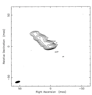
Figure 3.1 shows the image of Pictor A obtained from the data of 1991 March

(26)

16 P K S 0 5 1 8 - 4 5 8 , a pow erful, low red sh ift rad io g a la x y

Epoch frequency

(GHz)

Participating Telescopes

1991 March 12 2.3 Ds43,Pk,Hb,Na

1993 Feb. 18 8.4 Ds43,Pk,Hb,Na,Mr,Ht 1993 July 3 8.4 Ds43,Pk,Hb,Na,Mr,Prl5,Ht

Table 3.1: Observation log for PKS 0518—458.

Ds43 = Tidbinbilla (70 m), Pk = Parkes, Hb = Hobart, Na = Narrabri, Mr = Mopra, P rl5 = Perth (15 m), Ht = Hartebeesthoek

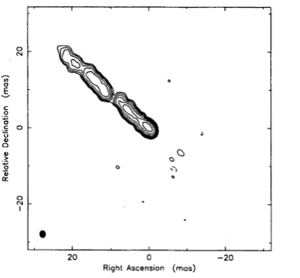
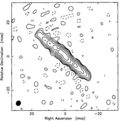
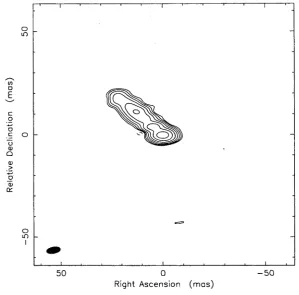
12, at 2.3 GHz. The source consists of a component which is extended toward the west at a position angle of approximately —77°. Figure 3.2 is an image resulting from observations on 1993 February 18 with a similar array of telescopes but with a higher resolution due to the higher observing frequency of 8.4 GHz. The bright component apparent at the eastern end of the source, when Figures 3.1 and 3.2 are compared, can be identified as the flat-spectrum core. In addition a jet-like structure extends to the west at a position angle of —79°.

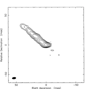
Figure 3.3 is an image produced from the data of 1993 July 3, at 8.4 GHz, but with resolution higher than Figure 3.2 due to the longer baselines to Perth available in the array for this observation. The core is again the brightest feature in the image and the jet is well resolved, revealing an extension from the core at a position angle of approximately —74°, with an angular length of approximately 7 mas, and a discrete component approximately 11 mas from the core, along the same position angle.

That the features in Figure 3.3 are real is supported by the fact that if the clean component model of Figure 3.3 is convolved with the restoring beam of Figure 3.2 then the reconvolved image and Figure 3.2 are identical.

The mismatch in frequency and resolution between the 2.3 GHz observations of 1991 March 12 and the 8.4 GHz observations in 1993 do not allow any mean ingful investigation of evolution in the pc-scale radio source over this period. The comparison of 8.4 GHz data between the 4.5 months 1993 Feb 18 to 1993 Jul 3 indicates that no significant structural change could be detected on that time-scale.

The data on baselines to Hartebeesthoek at 1993 February 18 and 1993 July 3 were sparse and not used during the imaging process. However, a significant detection of the source was made on both occasions. Approximately 0.2 Jy were detected on the Tidbinbilla to Hartebeesthoek baseline on 1993 July 3, correspond ing to an angular resolution of approximately 0.4 mas. Thus, a rough estimate of the radio core brightness temperature is 2 x l0 10 K at 8.4 GHz.

(27)

P K S 0 5 1 8 —4 58, a p o w erfu l, low red sh ift radio g a la x y 17

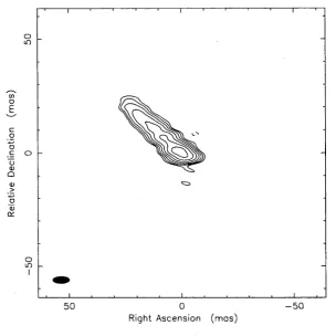
0518-458 o b s e r v e d a t 2.291 GHz. 1991 M ar 12

Right Ascension (mas)

Figure 3.1: Map peak, 1.0 Jy/beam. Contours, -0.5, 0.5, 1, 2, 4, 8, 16, 32, and 64% of peak. Beam FWHM, 24.5x9.7 mas @ -80°.

0518-458 o b s e r v e d a t 8 421 GHz, 19 9 3 F e b 18

(28)

18 P K S 0 5 1 8 —4 5 8 , a p ow erfu l, low red sh ift r a d io g a la x y

0 5 1 6 - 4 5 8 o b s e r v e d a t 8 .4 1 8 GHz, 1 9 9 3 J u l 03

10 p c

Figure 3.3: Map peak, 0.3 Jy/beam. Contours, -1, 1, 2, 4, 8, 16, 32, and 64% of peak. Beam FWHM, 1.9x1.6 mas @ -8.6°.

3.3 D iscu ssio n

The SHEVE observations have shown that the compact source at the nucleus of Pictor A has a core-jet structure approximately 10 pc in extent. A flat-spectrum core lies at the eastern end of the structure and a steep-spectrum jet extends toward the west, highly aligned with the kpc-scale jet and the western radio hotspot. In the highest resolution image the jet is resolved into an inner continuous jet and a detached component. Future VLBI observations of comparable quality and resolution will make an investigation of evolution in the pc-scale source possible.

Regardless, the pc-scale radio structure of Pictor A can be compared with existing high resolution optical observations.

The pc-scale core-jet radio structure aligns with a sub-arcsecond optical jet reported by Simkin, Robinson, and Sadler [1992] from narrow band HST imaging. They found that [OIII] emission frbTn the^ narrow line region of the Pictor A host galaxy is distributed in a roughly symmetrical fashion around the nucleus, while the line-free continuum takes the form of an elongated, jet-like structure aligned with the western radio lobe. They measure the optical jet to have dimensions of 50x220 mas.

On one hand, the coincidence of the optical jet with the pc-scale radio jet supports the suggestion of Simkin, Robinson, and Sadler [1992] that the optical jet is due to synchrotron emission.

(29)

P K S 0 5 1 8 - 4 5 8 , a p ow erfu l, low red sh ift r a d io g a la x y 19

good correspondence between radio and optical jets has been established, at least on kpc-scales. HST and radio imaging of the radio/optical jets in Virgo A and PKS 0521—365 [Sparks, Biretta, & Macchetto 1994; Macchetto et al. 1991) show a strong coincidence between the jet structure at radio and optical wavelengths.

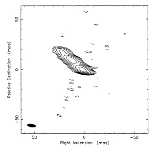
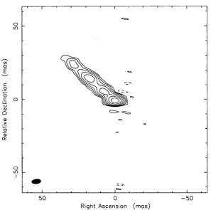
To show that the VLBI observations were not biased towards measuring a jet shorter than in reality, Figure 3.4 shows an image produced from simulated data. The data were simulated from the Caltech VLBI task FAKE using a source model which consisted of a 5 mas full width at half maximum (FWHM) circular Gaussian core component of 0.4 Jy and a 200 mas long and 50 mas wide constant surface brightness elliptical component of 0.7 Jy, orientated at a position angle of —77°. The source was given the RA and DEC of the Pictor A nucleus and “observed” at 2.290 GHz with the array of telescopes used on 1991 March 12. Realistic values for system temperatures, antenna diameters and antenna pointing were used to generate noise in the data. In Figure 3.4, the jet component can be easily detected to its full 200 mas extent, showing that the observations of 1991 March 12 would have been sensitive to a jet with the extent of the optical jet reported by Simkin, Robinson, and Sadler [1992].

sim u la te d m odel o b s e r v e d a t 2 .2 9 0 GHz, 1991 M ar 12

- 2 0 0

Right A scen sio n (m a s )

Figure 3.4: Map peak, 0.4 Jy/beam. Contours, -1, 1, 2, 4, 8, 16, 32, and 64% of peak. Beam FWHM, 32.5x13.3 mas @ -87.1°.

Thus, based on a simple synchrotron interpretation, the relationship between the VLBI observations and the HST observations is difficult to understand. A second epoch observation, with the post COSTAR HST, of the optical jet will be required before a detailed comparison between the optical and VLBI observations can be made.

(30)

20 P K S 0 5 1 8 —4 5 8 , a p o w erfu l, low red sh ift radio g a la x y

0."8x0."2 beam. This emission should be detectable and imagable with 2.3 GHz VLBI observations utilising an array similar to that used for Figure 3.1. With the higher bandwidth of the S2 VLBI system a better sensitivity to the hotspot emission will be possible. The resulting images would give a view of the interac tion between the jet and IGM at a resolution comparable to the HST observations. These observations have been proposed as future SHEVE experiments.

(31)

C h a p te r 4

C o m p a c t radio sou rces and 7 -ray

e m issio n

V L B I O b se rv a tio n s o f S o u th e r n E G R E T Id en tifica tio n s. I. P K S 0 2 0 8 - 5 1 2 , P K S 0 5 2 1 - 3 6 5 , an d P K S 0 5 3 7 - 4 4 1

Tingay, S.J., Edwards, P.G., Costa, M.E., Jauncey, D.L., Reynolds, J.E.,

Tziournis, A.K., Migenes, V., Gough, R., Jones, D.L., Preston, R .A., Murphy, D.W., Meier, D.L., van Omnien, T.D., St John, M., Hoard, D.W., Lovell, J.E.J., McCulloch, P.M., King, E.A., Nicolson, G.D., Wan, T.-S., & Shen, Z.-Q.

A c c e p te d to a p p ea r in T h e A str o p h y sic a l Jou rn a l (1996 J u n e 1 0 ).

4 .1

I n t r o d u c t io n

The first two dedicated gamma-ray astronomical satellites, SAS 2 and COS B, yielded between them one identified extragalactic source of greater than 100 MeV gamma-rays, the radio source 3C273 [Bignami & Hermsen 1983]. The Compton

Gamma-Ray Observatory ( CGRO) was launched in 1991 April. Of the four detec tors on board the Observatory, the Energetic Gamma-Ray Experiment Telescope (EGRET) is sensitive to the highest energy gamma-rays, those in the 20 MeV to 30 GeV range. To date, CGRO has discovered over 120 discrete sources of greater than 100 MeV gamma-ray emission.

Of these discrete sources the second EGRET Source Catalog, compiled from observations during phases I and II of the CGRO mission (from 1991 April to 1993 July), lists 40 high confidence identifications of strong, flat-spectrum extragalactic radio sources, and a further 11 marginal identifications [Thompson et al. 1995]. Identifications were classified as marginal if the candidate radio counterpart lies close to but outside the 95% uncertainty contour for the gamma-ray source posi tion. Previously, the high confidence and marginal classifications were based solely on photon statistics [von Montigny et al. 1995a]. To avoid confusion, the following terminology will be used here: strong and weak describe the statistical signifi cance of detection, and high-confidence and marginal describe the identifications. The rapid optical variability and large optical polarisation of many of the optical counterparts to the radio sources have resulted in their being classified as ‘blazars’.

The absolute gamma-ray luminosities for some EGRET sources are exceedingly high (~1048 ergs s-1, approximately the Eddington limit for a 1O1OM0 black hole)

(32)

22 C o m p a ct radio so u rces a n d 7-ray e m issio n

if isotropic emission is assumed. However, there are reasons for concluding that the emission is not isotropic. A number of the radio counterparts have already been observed with VLBI. These sources have generally exhibited apparent superluminal motions, suggesting beamed emission from relativistic matter travelling close to our line of sight. If the gamma-ray flux is also beamed along our line of sight then the luminosities derived by assuming isotropic emission will be overestimates.

The short time-scale variability of the gamma-ray emission from some of the stronger sources implies that the spatial extent of the gamma-ray emission region is on the order of 10 light days or less [von Montigny et al. 1995a].

From consideration of these two points it is generally postulated that the gamma-ray emission region lies within the base of the relativistic jet (c.f. references in von Montigny et al. 1995a).

The fact that many flat-spectrum radio sources have not been identified by EGRET and the assumption that the gamma-ray emission is beamed has been used to infer that the width of the gamma-ray beam is smaller than that of the radio beam, under a “unified scheme” where all bright, flat-spectrum radio sources are gamma-ray sources. Adopting a beam size for the radio emission of ~14° [Padovani & Urry 1992], Salamon &: Stecker [1994] derive a beam size for the gamma ray emission of ~4°. However, Dondi &; Ghisellini [1995] argue that the radio and gamma-ray beams may be collimated to the same extent and suggest that the EGRET sources have been detected because they are currently in a high state of gamma-ray emission, thus leaving undetected those sources currently in a low state of gamma-ray emission.

von Montigny et al. [1995b] have offered another alternative, which also relies on relativistic beaming, to explain why some radio sources have been detected in gamma-rays but others have not. von Montigny et al. [1995b] suggest that gamma- ray sources may have jets which remain straight from the scale of the gamma-ray emission region all the way to the kpc-scale and that we lie within the gamma-ray beaming cone as well as the radio beaming cone. On the other hand, jets which bend allow for the possibility that the gamma-ray emission is beamed away from our line of sight but that we still lie within the beaming cone of the radio emission. The implication of this suggestion is that the majority of gamma-ray loud sources have closely aligned small and large-scale jets whereas the majority of gamma-ray quiet sources have misaligned small and large-scale jets.

Indicators of relativistic beaming are therefore very relevant for models of the gamma-ray emission. For example, the models proposed by Salamon & Stecker [1994] and Dondi &; Ghisellini [1995] make quite different predictions about the distribution of line of sight angles of the relativistic jet in EGRET sources. Salamon & Stecker predict that all gamma-ray sources have their jets aligned within 4° to the line of sight whereas Dondi & Ghisellini imply a broader distribution of angles to the line of sight.

(33)

C o m p a c t ra d io so u rces and 7-ray em issio n 23

Thus, the three aims of the work described in this chapter are:

1] To in c r ea se th e n u m b ers o f E G R E T -id e n tified ra d io so u rces w ell s tu d ie d w it h V L B I by ta r g e tin g th o se in th e S o u th e r n H e m isp h e r e .

2] To b e g in to b u ild a sa m p le o f stro n g , fla t-sp e c tr u m radio so u rces w h ich h a v e n o t b e e n id en tified by E G R E T b u t are o th e r w is e sim ila r to th e E G R E T -id e n tifie d so u rces, as a co m p a riso n sa m p le.

3] To c o m p a r e th e r e la tiv is tic b e a m in g in d ica to rs d e r iv ed for th e so u rces p r e se n te d h ere from 1] an d 2], and also for o b se rv a tio n s from th e lite r  a tu re .

To meet these aims, this chapter describes the first VLBI observations of three EGRET-identified radio sources, PKS 0208—512, 0521—365 and 0537—441, all high-confidence identifications in the second EGRET catalog. Also described are the first high-resolution VLBI observations of four radio sources which have not been identified by EGRET, but show evidence for blazar activity, PKS 0438—438, PKS 0637—752, PKS 1514—241, and PKS 1921-293. In § 4.2, a brief discussion of the beaming indicators which can be estimated from VLBI observations is given. In § 4.3, the data reduction and analysis methods specific to this work are outlined. The results for each individual source are presented in § 4.4, where estimates of the radio core brightness temperatures and pc-scale to kpc-scale misalignment an gles are made. A discussion and comparison of the VLBI properties of the sources considered in § 4.4, as well as other radio sources from the literature, is given in § 4.5.

4.2 Indicators o f relativistic beam ing

Relativistic beaming can be measured in terms of the Doppler factor, 5, which relates the intensity in the observer’s frame to the intensity in the rest frame, of radiation originating from material travelling at a significant fraction of the speed of light.

s * = s3 -q = 1 = ( l - / 3 2) ^

S r e s t ; --- — - ^3_ -q ( 1 _ ßCOs0)3~a ( 1 - ßcos0)3~a

for a spherical component, where 7 and ß have their usual definitions in relativity and refer to the motion of the radiating material (e.g. Blandford and Konigl 1979).

6 is the angle the material motion makes to the line of sight and a (S oc va) is the spectral index of the emission.

Another relativistic effect, apparent superluminal motion, can be observed when a source of radiation is moving at a substantial fraction of the speed of light and in a direction close to the observer’s line of sight,

a _ ßsin6 l app = 1 - ßcosO ’