Some reflections on the building and calibration of useful network models

Some Reflections on the Building and Calibration of Useful

Network Models

R. Burrows

Department of Civil Engineering, University of Liverpool

T.T. Tanyimboh

Department of Civil Engineering, University of Liverpool, UK

M. Tabesh

Department of Civil Engineering, University of Tehran

Abstract

Over the past 10 years or so in the UK much effort has gone into the construction of computerised network models of water supply and distribution networks. At best such models offer an approximation of reality, their performance in simulation being constrained, in many cases, by the uncertainties present in the data upon which they were compiled. Most notable are the problems of demand specification, including leakage evaluation. In the UK this exercise is compounded by the unmetered nature of most domestic consumption. Reconciliation of the output of this process is invariably and inextricably linked to such matters as flow-meter accuracy, network and district metered area (DMA) connectivity, and monitored pressure regime, as well as precision in property allocation and quality of billing records. For large networks the task of the modeller is most arduous since the exercise of pipe calibration, leading to production of the ‘verified’ model, is itself highly dependent upon the distribution of flows generated in the network. The paper elaborates on these problems and introduces outlines for systematic treatments of the data reconciliation processes, with the aim of producing usable models which ‘best’ represent reality from the information available.

Keywords: Water distribution, Network models, demand.

1. INTRODUCTION

This contribution focuses on the characterisation of demand for network modelling studies. It draws from a sample network model study completed for a medium sized town in the UK. DMA level analysis from field survey data and customer accounts records, together with pipe system, asset and operational data, as well as the resulting calibrated WATNET [1] network model, are utilised in the exploratory approaches described. Standard minimum night flow (MNF) methods are used for leakage evaluation and the estimation of unmetered consumption, and discussion then centres on their reliability, the underlying uncertainties and their implications.

based on minimisation of residuals in zonal flow balances consistent with constraints imposed on deviations from expected levels of consumption/leakage and hydraulic factors. It does not at this point extend to the pipe-by-pipe calibration process, where synthesised pressures and flows are fitted to monitored field data. Recent advances in this area have recently been presented at the CCWI 2000 Conference [2]. It is envisaged that both procedures might be run in conjunction for most effective anomaly detection.

2. LEAKAGE ESTIMATION AND DEMAND ALLOCATION

Hydraulic network models have yet to be fully integrated into the operational management and strategic functions of many water companies. Whilst such models have been constructed widely, PCC and leakage figures specified at DMA level resulting from model building and calibration studies are potentially error prone. The aimhere is to improve quality control on such estimates and their diurnal variations. By way of outline, levels of PCC and leakage and their profiles are first critically evaluated from an earlier sample case study.

The normal procedure in network model building is to select a single data set from one day during the fieldwork study. Using a DMA level approach, domestic unmetered consumption (the largest component) is obtained as the residual of a flow balance calculation involving: net meter inflow/outflow figures; metered consumer average demands (and profiles, representing the variation over 24 hours); and leakage obtained from Minimum Night Flow (MNF) analysis. For these calculations the leakage profile adopted may be: a standard (such as the stepped WRc profile where night-time losses are 1.1 times daily average and daytime losses 0.9 times, with a so called ‘T’-factor ~ 20 hours, which converts this maximum (night-time) leakage rate to the total daily loss); or a zone (DMA) specific profile linked to pressure variations, possibly based on average zone pressures through the Leakage Index relationship [3, 4], LI = 0.5 x AZP + 0.0042 x AZP2, where AZP is the average zone pressure, the weighted mean pressure in the distribution mains.

Note that the current generation of network models are not capable of active self adjustment of leakage (or consumption) in accordance with prevailing pressures during a simulation, since they are ‘demand’ and not ‘head’ driven. This leakage evaluation may therefore need to be solved interactively with the network modelling if AZP is to be applied with maximum rigour. Tanyimboh et al [5, 6] have recently discussed the practicability of head-driven simulation.

A high level of uncertainty must be expected when basing demand allocation on only a single set of data, both in terms of the leakage figures arising and the scale of PCC and its diurnal profile. The virtue of the approach is that it recreates the observed flows closely, so enabling unhindered model calibration. This is a virtue, however, only if the flows themselves were accurate! Outputs from a sample study area involving a town with 31 DMAs are shown in Figure 1 [7]. This shows variations in PCC, as well as levels of leakage, beyond that which might be considered intuitively reasonable.

Figure 1 Per capita consumption and leakage figures arising from the model building case study

more readily accepted if they were populated with realistic demand profiling throughout and if they were able to take into account the routine high quality leakage monitoring now becoming the norm within the UK water industry.

A better approach, therefore, is to utilise the latest data available (at the time of the modelling study) at company/network/DMA levels, to constrain component demands to lie within chosen bounds about the expected values. To then integrate these constraints on the DMA level demands with the Flow Balance and basic Data Reconciliation processes. From this holistic approach, the underlying uncertainties in the problem can be accounted for by systematic means, ie minimising flow balance residuals across the network. A best estimation approach is suggested here and is illustrated in the next section with an application based on demand characterisation based on the early WATNET (for DOS) approach [1], where 5 specific categories of nodal demand could be stipulated.

This provides a holistic treatment of:- data reconciliation; pipe connectivity investigation; flow balance; leakage evaluation; and demand allocation. It employs optimisation to account for uncertainties in the various items of data, within accepted bounds, by minimising flow balance errors over 24hrs. By allowing for measured flow data inaccuracy and constraining consumption estimates it yields the most likely parameter values compatible with the source data. As an extension the process could be operated in conjunction with network model calibration, for more effective resolution of anomalies.

3. DATA RECONCILIATION USING A BEST PARAMETER ESTIMATION TECHNIQUE

As an initial estimate of uncertainty in the water system's elemental consumptions, leakage and hydraulic performance, a value of residual flow can be defined, as follows, for each zone [8].

Rest = Net inflowt - (Tt,1 + Tt,2 + Tt,3 + Tt,4 + Tt,5) (1)

where Rest is the residual at each time step, Net inflow is the metered inflow

minus any metered outflows. Tt,1 to Tt,5 are the five types of consumption

permitted in 'WATNET', and subscript t (from 0 to 23) refers to time (hrs.)

0 1 2 3 4 5 6 7 8 No. zones 2 5 5 0 7 5 1 0 0 12 5 1 5 0 1 7 5 2 0 0 2 2 5 20 0 0

PCC l/h/d

Notown 0 1 2 3 4 5 6 No. zones 1 0 2 0

30 40 50 60 70 80 90

1

0

0

Leakage %

For each elemental consumption type, the following percentage errors might be considered to encompass the range of uncertainty or inaccuracy in the base data for this pilot study.

1) ± 5% error for all flow measurements (i.e. inflows/outflows to the zone) to cover the range of instrument inaccuracies.

2) ± 5% error for all metered consumer elements, Types 2-4, obtained from consumer accounts records. This range of variation is perceived as representing possible day to day variability in metered consumption as well as seasonal drifting. These error margins are necessary since it is impracticable to monitor all metered consumers during a typical fieldwork study.

3) ± 10% error for values of pressure dependent leakage based on the MNF method. This range is incorporated to account for the uncertainty in the relationship between leakage and zone pressure and its integration in the MNF calculation.

4) ± 25% variation in values of domestic unmetered (u/m) consumption (Type 1). This makes allowance for the fact that PCC may be expected to vary, to some degree, from zone to zone, partly as a result of socio-economic factors.

A later refinement could be to build in an explicit link between PCC and socio-economic make up, possibly through the 'ACORN' categorisation system or from application of micro-simulation [9]. In each individual zone or DMA, minimisation of the sum of the squares of the residual in equation (1) over the full set of snapshot times, representing the objective function (F) would produce the 'best' parameterisation by application of formal optimization methods.

Normally, in the process of data collection in the field, however, the values of the net inflow are obtained from differences between the total inflows to, and outflows from the zone. It is assumed that all the other connections to adjacent zones are cut off by the closed status of boundary valves. In reality it is possible that some of these valves may not be closed completely and other connections or valves may have been overlooked and, consequently, water could be passing from them. Obviously, this would disturb the balance equation in these zones and the methodology can be extended to consider this possibility of unknown flow passing between adjacent zones taking account of hydraulic head factors.

To simulate this possible inter-connectivity an additional term is added to the objective function. This assumes that the flow can pass from one zone to an adjacent zone with lower average total head, according to the diurnal variations of the average total head differences between each pair of adjacent zones. With this extension the objective function is minimised over all zones (NZ) in the chosen hydraulic area.

3.1 Optimization Procedure

(

)

∑

∑

∑ ∑

t ;where Res a x H H x

s Re F

Minimize (2)

0.95 ≤ xi,1≤ 1.05; 0.75 ≤ xi,2 ≤ 1.25; 0.95 ≤ xi,3 , xi,4 , xi,5≤ 1.05; 0.90 ≤ xi,6 ≤ 1.1;

0.0 ≤ xi,7 ≤ 1.1 x TMNFT,5 and

(

)

m ,i

i m

,i

H inflow Net Ave. x

0

∆ ≤

≤ (3)

Whilst satisfying:-

(i) The MNF calculation is,

∑

∑

= =

= −

+

7

1 j

k

1 m

i m

,i m , MNFT j

, MNFT j

,i j ,

MNFTj .x (H H ).x LOUC

a (4)

where, at,1 = Qt,0 (net inflow); at,2 = -Tt,1 (domestic demand); at,3 = -Tt,2 (small trade

consumptions); at,4 = -Tt,3 (10 hrs. industrial activities); at,5 = -Tt,4 (24 hrs. industrial

activities); at,6 = -Tt,5 (leakage); at,7 = 1 at t =MNFT, else 0; Ht,i and Ht,m are average total

heads in zones i and m.

Furthermore, x7 represents the optimum leakage value at minimum night flow time

(MNFT) and LOUC (here taken as 1.0 or 1.7 l/hr/prop. x number of unmetered properties), is the normal household night flow allowance. Note that aMNFT,2and aMNFT,6 are set zero in

the MNFT constraint to satisfy the flow balance equation at MNFT. This constraint produces the value of unaccounted for water at the MNF condition, i.e. UFWM. In some zones with no domestic demand (Tt,1), e.g. pure industrial zones, the MNFT constraint is

eliminated because the concept of ‘minimum night flow’ is not meaningful in such situations.

(ii) For the unknown passing flows

xi,m - xm,i = 0 ; over all adjacent zones (5)

and xi,m = Qi,m / H∆ i,m (6)

is a variable to account for the unknown passing flow (Qi,m) between two adjacent zones i

and m and H∆ i,m = daily average of total head difference between two adjacent zones i

and m.

To calculate the optimum values of flows and consumptions, a computer programme has been developed using a least squares minimization methodology (E04NCF) from the NAG Fortran library [10].

3.2 Implementation

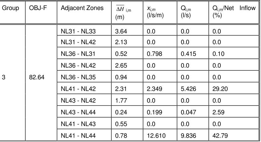
Values of total head within each zone were produced by a 'WATNET' hydraulic flow model calibrated and verified from field data in this case. From this the daily average of total head for each zone has been calculated. In the normal situation this information may be available from field data. For the optimisation, Qi,m representing the average daily

according to PCC and leakage figures arising from the standard analyses. To account for all the adjacent zones, some zones were considered in more than one group [11].

It is worth noting that consideration of the network in sub-groups helps to simplify the problem by reducing the size of the objective function (F) and the number of variables. Consideration of the entire network in only one group leads to a complicated problem, with more than 230 variables in this case study.

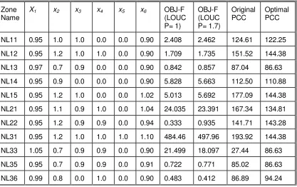
Table 1: Results of optimisation at single zone (DMA) level.

Zone Name

X1 x2 x3 x4 x5 x6 OBJ-F

(LOUC P= 1)

OBJ-F (LOUC P= 1.7)

Original PCC

Optimal PCC

NL11 0.95 1.0 1.0 0.0 0.0 0.90 2.408 2.462 124.61 122.25

NL12 0.95 1.2 1.0 1.0 0.0 0.90 1.709 1.735 151.52 144.38

NL13 0.97 0.7 0.9 0.0 0.0 0.90 0.842 0.857 87.04 86.63

NL14 0.95 0.9 0.0 0.0 0.0 0.90 5.828 5.663 112.50 110.88

NL15 0.95 1.2 1.0 0.0 0.0 1.02 5.013 5.692 177.09 144.38

NL21 0.95 1.1 0.9 1.0 0.0 1.04 24.035 23.391 167.34 134.81

NL22 0.95 1.2 0.9 0.9 0.0 0.94 0.333 0.935 141.71 143.28

NL31 0.95 1.2 1.0 1.0 1.0 1.10 484.46 497.96 193.92 144.38

NL33 1.05 0.7 0.9 0.9 0.0 0.90 21.499 18.097 27.44 86.63

NL35 0.95 0.7 0.9 0.9 0.0 0.91 0.722 0.771 85.02 86.63

NL36 0.99 0.8 0.0 1.0 0.0 0.90 0.483 0.412 86.89 94.24

Table 1 shows sample results for the optimisation applied to individual zones. The 'Original PCC' is the outcome from the conventional MNF calculations applied to each DMA in turn, the 'Optimal PCC' arises from applying the network average value (122l_/h/d)

into the optimisation. Values of x1 – x6 indicate the adjustment factors, within the

stipulated uncertainty ranges, which minimise the flow balance error for that zone. High values of the objective function (OBJ-F) signify zones where the data does not reconcile adequately, note especially NL31 and NL33, suggesting perhaps that boundary valves are not tight (the zone is not ‘operable’) or that there are errors in base data. These zones would be prioritised for re-evaluation and, probably, a repeated field work survey.

Table 2: Values of xi,m and Qi,m for adjacent zones from multi-zone optimisation.

Group OBJ-F Adjacent Zones _∆Hi,m

(m)

xi,m (l/s/m)

Qi,m

(l/s)

Qi,m/Net Inflow

(%)

NL31 - NL33 3.64 0.0 0.0 0.0

NL31 - NL42 2.13 0.0 0.0 0.0

NL36 - NL31 0.52 0.798 0.415 0.10

NL36 - NL42 2.65 0.0 0.0 0.0

3 82.64 NL36 - NL35 0.94 0.0 0.0 0.0

NL41 - NL42 2.31 2.349 5.426 29.20

NL43 - NL42 1.77 0.0 0.0 0.0

NL43 - NL44 0.24 0.199 0.047 2.59

NL41 - NL43 0.55 0.0 0.0 0.0

NL41 - NL44 0.78 12.610 9.836 42.79

Table 3: Optimum values of variables arising from the optimisation of Table 2.

Zone Name

x1 x2 x3 x4 x5 x6

NL31 0.95 1.25 1.05 1.00 1.05 1.00

NL33 0.95 1.00 1.00 1.00 0.00 1.10

NL35 0.95 0.75 0.95 0.95 0.00 1.10

NL36 0.95 1.25 0.00 1.00 0.00 1.00

NL41 0.95 1.25 0.95 0.00 1.05 0.90

NL42 0.95 1.00 1.00 1.05 0.00 1.00

NL43 0.95 1.00 0.95 1.00 0.00 1.00

NL44 0.95 1.00 1.00 1.05 1.05 1.00

4. TRUNK MAIN LEAKAGE

only to weak ‘indicators’ of the sources of discrepancy. Interpretation, therefore, becomes highly intuitive and subjective.

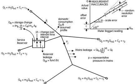
The underlying concept advocated here, and depicted in Figure 2 is to utilise all available data in a systematic manner in an attempt to explain flow balance discrepancies, whilst making allowance for the uncertainties associated with individual flow meter data streams, as well as relevant physical properties (ie service reservoir/tank dimensions). Other relevant information such as reservoir/tank level data (and its errors) and any pipeline pressure data (variations in which will affect trunk main leakage) can be included also. The data would be analysed for the flow residual (discrepancy) hour by hour, or more frequently if available, ie on the 15 minute scanning cycle of much instrumentation, and extended across a suitably long period of recording. By this means, variations in the time traces of the component data are maximised so enabling interrogations for correlation studies between: the ‘pattern’ of the flow discrepancy and corresponding pattern of an individual meter reading, which might indicate a meter error; or between the pattern of the discrepancy and the pipeline pressure fluctuations, which might then indicate mains leakage. Such visual interrogation of time traces is often undertaken as part of the data reconciliation in network modelling studies. Unfortunately, in the most likely situations where the flow discrepancy is explained by the accumulation of errors in a number of the meters together with some trunk main leakage, it becomes a highly intuitive, unreliable and time consuming task, the complexity being beyond the scope of brainpower alone.

Figure 2 Schematic of a trunk main with metered inlets/outlets: flow balance over increment _∆t

pressure regime. As envisaged at this point, the uncertainties of the problem would be treated as follows:-

(i) Each meter input field would have assigned to it measures of its error (ie unknown ‘offset’ (c) and ‘scale’ (m) errors and possibly allowance for random resolution error, by this means a tendency for error to increase with flow magnitude would be accommodated, for example).

(ii) Unknown trunk main leakage at a given pressure, (Ql_{) would be required to} vary in accordance with changes in pressure according to a suitable power law (ie N1).

(iii) Unknown consumption off the mains could also be accommodated by setting an assumed average value (Qp) and assigning an appropriate (estimated) time profile

(iv) Reservoir may have errors in plan (ma) and level recordings (c and m)

The mathematical problem now becomes one of identifying the values of the unknown parameters, such that the flow balance residual is minimised (when summed for all times in the data records). These unknowns are:- the c and m terms for each meter and reservoir level, the m value for each tank, and the domestic Qp and leakage Ql terms. Clearly, the reliability of the outcome will be partly dependent on the size of the data set of flow balance snapshots (for sampling at 15 minute intervals, this would amount to close to 700 per week) as well as other features of the input data. The formulation would be, referring to Figure 2,

Minimise

2

t all

5

2 k

LRt Rt t pt kt t

1

T Q (Q ) Q Q Q Q

F

∑

∑

=

− − − − −

= l (7)

At best the method should give the most likely scale of trunk main leakage (where meter reliabilities are high and errors small but not insignificant relative to the leakage term). At worst, the approach will yield estimates of c and m for each meter, the departures from (zero) and (1), respectively, being strong indicators of unreliability and so guiding further action in reconciling the anomalies.

The approach is analogous to the earlier uncertainty based methodology for reconciliation of distribution zone or District Metered Area (DMA) leakage, demand and consumption data which also draws on the meter flows used in the trunk mains analysis. It would perhaps be appropriate to broaden the study so as to enable this additional level of reconciliation on the DMA meter flows (described in Section 3) to be integrated into the evaluation of the trunk main problem.

5. CONCLUDING COMMENT

The approaches outlined offer a means of integrated and systematic data reconciliation for problems beyond the scope of ad hoc intuitive manual actions. Operated as a data pre-processor they focus attention to zones which are potentially anomalous, necessitating further fieldwork studies.

Populating network models with the outputs from the above analyses and so running calibration studies with a degree of overlap, would provide the most robust basis for their routine use in operational or planning studies.

6. REFERENCES

[1] WRC plc. (1992) 'Analysis, simulation and costing of water networks and a guide to WATNET 5.3 computer program', WRC plc, Swindon, UK.

[2] Savic D and Walters G. (1999) 'Water industry systems: modelling and optimization applications', (Vol. 1, Part IV - Model Calibration), Research Studies Press, Herts., England, ISBN 0863802486.

[3] WRC plc Technical Working Group on Waste of Water. (1980) 'Leakage control, policy and practice', National Water Council Standing Technical Committee, Report No. 26, WRC plc, Swindon, UK.

[4] WRC plc Engineering and Operations Committee. (1994) 'Managing leakage', UK, Water Industry, WRC plc, Swindon, UK.

[5] Tanyimboh T T, Burd R, Burrows R and Tabesh M. (1999) 'Modelling and reliability analysis of water distribution systems', Wat. Sci. Tech., Vol. 39, No. 4, 249-255.

[6] Tanyimboh T T, Tabesh M and Burrows R. (2000) 'An appraisal of the source head methods for calculating the reliability of water distribution networks', in 'Management of Water Distribution and Leakage Control', EPSRC Short Course, University of Liverpool, March, 19-23 (under review for ASCE J. Water Resources, Planning & Management).

[7] Tabesh M and Burrows R. (1995) ‘Investigation on aspects of water consumption and system leakage in the UK’, Int. J. Water Resources Engineering, Vol. 13, No. 1, 1995, 35-46.

[8] Tabesh M, Burrows R and Tanyimboh TT. (1996) ‘Water consumption and network leakage evaluation using a best parameter estimation technique’, in Hydroinformatics’96, Muller (ed), Balkema, Rotterdam, 387-394.

[9] Williamson P, Clarke G P and McDonald A T. (1996) 'Estimating small-area demands for water with the use of microsimulation' in "Microsimulation for Urban and Regional Policy Analysis" ed. Clarke G P, Pub. Pion, London, 118-148.

[10] NAG Ltd. (1991) 'NAG fortran library mark 15', The Numerical Algorithms Group Ltd, 4.