Orbits in a generalized two-body problem

McInnes, C.R. (2003) Orbits in a generalized two-body problem. Journal of Guidance, Control and

Dynamics, 26 (5). pp. 743-749. ISSN 0731-5090

http://eprints.cdlr.strath.ac.uk/

6246

/

Strathprints is designed to allow users to access the research output of the University

of Strathclyde. Copyright © and Moral Rights for the papers on this site are retained

by the individual authors and/or other copyright owners. You may not engage in

further distribution of the material for any profitmaking activities or any commercial

gain. You may freely distribute both the url (

http://eprints.cdlr.strath.ac.uk

) and the

content of this paper for research or study, educational, or not-for-profit purposes

without prior permission or charge. You may freely distribute the url

(

http://eprints.cdlr.strath.ac.uk

) of the Strathprints website.

Orbits in a Generalized Two-Body Problem

Colin R. McInnes¤

University of Glasgow, Glasgow, Scotland G12 8QQ, United Kingdom

The two-body problem is a well-known case of the general central force problem with an attractive, inverse square force. However, there are forms of spacecraft propulsion, such as solar sails and minimagnetospheric plasma propulsion, which generate a repulsive, inverse square force. Because this force can be modulated, a more general central force problem is then formed. Such a problem is investigated and the families of orbits available using both forward integration and an inverse approach are explored. Both are used to explore various modes of transfer between circular coplanar orbits and to determine strategies for escape.

Nomenclature

a = orbit semimajor axis e = orbit eccentricity G = gravitational constant

h = speciŽ c orbital angular momentum m = mass

r = orbit radius T = orbit period t = time

u = inverse of orbit radius W = Wronskian

¯ = lightness number

µ = polar angle

¸ = spiral parameter

¹ = gravitational parameter,G.m1Cm2/

¿ = transfer duration

! = argument of perigee

Introduction

B

propulsion2 _{(M2P2) generate thrust-induced forces that vary}

as the inverse square of heliocentric distance (as do so-called mag-netic sails3_{/. For a solar sail, a Ž xed-sail area will intercept a  ux}

of photons that diminishes as the inverse square of heliocentric dis-tance, whereas for M2P2 propulsion, the power available to drive the system diminishesas the inverse square of heliocentricdistance. (Although an M2P2 system using a nuclear power source would provide constant thrust.) The M2P2 system provides an essentially radial thrust as its magnetic Ž eld de ects the solar wind plasma, whereas a large, high-performancesolar sail is well suited to deliv-ering a radial thrust because sun pointing can be achieved passively if the sail has a slightly conicalform with the apex directedsunward. This is a different mode of operation from articulatedsolar sails that can direct the sail thrust vector within 90 deg of the sun line. How-ever, high performancesails may be unsuited to such articulationto minimize loads on their gossamer structure.

In addition to the inverse square form of these propulsive forces, the thrust magnitude can in principle be modulated between limits. For the M2P2 system, the thrust can be modulated by in ating or de ating its bubble of magnetic Ž eld, whereas a solar sail can in principle alter its effective area. This can be achieved by partly restowingthe sail, or rotatingpanelsof a segmentedsail. More likely,

Received 10 October 2002; revision received 11 March 2003; accepted for publication 16 April 2003. Copyright°c 2003 by Colin R. McInnes. Published by the American Institute of Aeronautics and Astronautics, Inc., with permission. Copies of this paper may be made for personal or internal use, on conditionthat the copier pay the $10.00 per-copy fee to the Copyright Clearance Center, Inc., 222 Rosewood Drive, Danvers, MA 01923; include the code 0731-5090/03 $10.00 in correspondence with the CCC.

¤_{Professor, Department of Aerospace Engineering; colinmc@}

aero.gla.ac.uk.

for a high-performance spin-stabilized disk sail, a variation of the coning angle of the angular velocity vector will lead to an averaged, modulated radial thrust. The main constraint on such systems is that the inverse square thrust is always directed along the sun line, radiallyaway from the sun. In addition,therewill be some maximum available thrust available, determined by the sail area or the M2P2 sizing.

The dynamicsof low-thrustpropulsionwith constantradial thrust has previously been considered by a number of authors.4¡8 _Here,

the related problem of a modulated, inverse square radial thrust is posed and solved with speciŽ c application to solar sail and M2P2 propulsion. As will be seen, large families of orbits can be inves-tigated using analytical methods resulting in both closed and open orbits. The general central force problem with the force scaling as rN_{(integerN/has long been investigated,for example, see Ref. 9.}

Here, however, we present the thrust modulation as a function of polar angle and exploit such general force laws for speciŽ c applica-tions such as orbit transfer.Although there is clear applicationof the open orbits to escape missions, such as fast trips to the heliopause,10

closed orbits may also Ž nd applicationsfor space physics missions that monitor and explore the structure of the solar wind plasma.

Central Force Problem

The equationsof motionfor a spacecraftwith a modulated,inverse square radial thrust may be written in plane polar coordinates (r; µ) as1

R

r.t/¡r.t/µ.P t/2_{D ¡[1¡¯.µ /]} ¹

r.t/2 (1a)

1 r.t/

d dt[r.t/

2_{µ.P t/]D0 (1b)}

wherer.t/is the heliocentric distance of the spacecraft (m2/from

the sun (m1/andµis the polar angle of the spacecraft, measured

anticlockwise from some reference direction, as deŽ ned in Fig. 1. Because both the spacecraft thrust and solar gravity have an inverse square variation, the induced thrust can be parameterized by the lightness number¯, deŽ ned as the ratio of the thrust force to solar gravitational force acting on the spacecraft. For the case of a solar sail, a sail with a Ž xed surface area will have a constant lightness number, whereas for M2P2 propulsion,a Ž xed input power will also lead to a constant lightness number. However, the effective sail area and M2P2 thrust can be modulated, so that¯can be a function ofµ, with the constraintthat 0·¯· Q¯where¯Qis the maximum lightness number attainable.

The equations of motion may now be reduced because a central force problem is still being considered, and so orbital angular mo-mentum is conserved. Integrating Eq. (1b) yieldsr2_µP_{Dh, whereh}

is the speciŽ c orbital angular momentum. Then, Eq. (1a) may be written as

R

r.t/¡h2_=r.t/3_{D ¡[1¡¯.µ /][¹=r.t/}2_{] (2)}

744 MCINNES

Fig. 1 Central force problem.

When the substitutionu.µ /D1=r.µ /is made, and conservation of angular momentum is used to change the independentvariable from timetto polar angleµ, it can be seen that Eq. (2) is transformed to

u00_{.µ /Cu.µ /D.¹=h}2_{/[1¡¯.µ /] (3)}

where the prime indicates a derivative with respect to polar angleµ. Because¯.µ /can be speciŽ ed a priori,with the constraint0·¯· Q¯, Eq. (3) can in principle be solved in closed form to determine the resulting spacecraft orbitr.µ /. To solve Eq. (3), the associated ho-mogeneous equation, deŽ ned by

u00_{.µ /Cu.µ /D0 (4)}

must be solved. The general solution of this homogeneous equation uH.µ /is then given by

uH.µ /DC1u1.µ /CC2u2.µ / (5)

whereC1andC2are arbitrary constants,determined from the initial

conditionsof the problem, andu1.µ /andu2.µ /are

linearlyindepen-dent solutions to Eq. (4). It is clear that two solutions to Eq. (4) are u1.µ /Dcosµ andu2.µ /Dsinµ, the fundamental set of solutions

to Eq. (3). The linear independenceof these two solutions,although clear, can be veriŽ ed by calculating the WronskianW.µ /so that

W.µ /D

­ ­ ­ ­

u1.µ / u2.µ /

u0

1.µ / u02.µ /

­ ­ ­

­D1 (6)

Given that Eq. (3) has no dependence on u0_{.µ /, it is expected}

thatW0_{.µ /D0. Now that the general solution to the associated}

homogeneous equation has been determined, the general solution to Eq. (3) can be found by Ž nding a second, particular solution uP.µ /. This particular solution can be found using the method

of variation of parameters, by proposing a solution of the form uP.µ /Dv1.µ /u1.µ /Cv2.µ /u2.µ /. It can be shown that the unknown

functionsv1.µ /andv2.µ /must satisfy

v0

1.µ /u1.µ /Cv02.µ /u2.µ /D0 (7a)

v0

1.µ /u01.µ /Cv02.µ /u02.µ /D.¹=h2/[1¡¯.µ /] (7b)

When it is noted thatW.µ /D1, the solution to this set of simulta-neous, Ž rst-order differential equations is then given by

v1.µ /D ¡_h¹₂

Z

u2.µ /[1¡¯.µ /] dµ (8a)

v2.µ /D _h¹₂

Z

u1.µ /[1¡¯.µ /] dµ (8b)

so that the particular solution to Eq. (3) may be written as

uP.µ /D ¡_h¹₂u1.µ /

Z

u2.µ /[1¡¯.µ /] dµ

C_h¹2u2.µ /

Z

u1.µ /[1¡¯.µ /] dµ (9)

Finally, the general solution to Eq. (3) is given byu.µ /DuH.µ /C

uP.µ /so that

u.µ /DC1cosµCC2sinµ¡_h¹₂ cosµ

Z

sinµ[1¡¯.µ /] dµ

C_h¹₂ sinµ

Z

cosµ[1¡¯.µ /] dµ (10)

For closed periodic orbitsu.µ /, the orbit periodT can now be ob-tained, deŽ ned here as the time between successive periapsis pas-sages (atµO andµP/. The orbit period can be obtained in closed form by a quadrature usingr2_µP_{Dhso that}

T D 1_h

Z _µP

µO

dµ

u2_{.µ /} (11)

If¯.µ /is now deŽ ned from a large class of elementary functions, the integrals in Eq. (10) can be performed andu.µ /obtained and, thus, so can the orbitr.µ /.

For example, if the lightness number is modulated according to

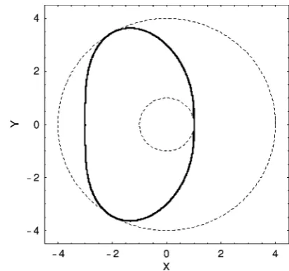
¯.µ /D cos2_{µ, so that 0·¯·1, the described methodology yields}

u.µ /D.uO=6/[3C.6C1=uO/cosµCcos 2µC.6C2=uO/sinµ]

(12)

Then, if the initial conditionsof the problem are chosen such that the spacecraftbeginson a circularorbitwithu.0/DuOandu0.0/D0, so

that¹=h2_Du

O, the constants are found to beC1Du0=3 andC2D0.

Therefore, becauseuOD1=rO, whererOis the initial circular orbit

radius, andr.µ /Du.µ /¡1, it can be seen that the resulting orbit is deŽ ned by

r.µ /D _{3C2 cos}6rO

µCcos 2µ (13)

whererO·r.µ /·4rO, as shown in Fig. 2. The orbit period is then

obtained from Eq. (11) as

T D¡r32

O

¯_p

¹¢£334p2¡3Cp3¢_¼¤ (14)

It has been shown then that the classical two-body problem can be extended to a more generalized central force problem applicable to

spacecraft that are able to generate an inverse square radial, mod-ulated thrust. If the spacecraft lightness number can be deŽ ned as a function of polar angle, the resulting orbit and orbit period can in general be determined in closed form. Applications to both solar sail and M2P2 propulsion will be explored later.

Inverse Problem

Now that the forward integration problem has been investigated and solved,the inverseproblem will be considered.From Eq. (3) it is clear that, ifu.µ /is sufŽ ciently smooth, then the required functional form of the lightnessnumber can be determinedin closed form using

¯.µ /D1¡.h2_=¹/[u00_{.µ /Cu.µ /] (15)}

Therefore, with the constraint 0·¯· Q¯imposed, large families of orbitscan be deŽ ned a prioriand the requiredlightnessnumber mod-ulation determined using Eq. (15). The key constraint on Eq. (15) is that¯¸0. Again, if it is assumed thatu.0/DuO andu0.0/D0,

then¹=h2_Du

O, which implies that

u00_{.µ /Cu.µ /·u}

O (16)

This constraint will be used later to determine bounds on admissi-ble orbits that possess the property that¯¸0. Now that the inverse problem has been deŽ ned, several individual cases will be consid-ered.

Circular Orbit

For a closed circularorbit of radiusR, the orbit equationis simply r.µ /DRso that Eq. (15) yields

¯D1¡h2_{=¹R (17)}

It can be seen that the minimum distance at which a circular orbit can be sustained is constrained by the orbit angular momentumh. Therefore, in order that¯¸0, it is clear that there is a minimum orbit radius such thatR¸h2_{=¹. The orbit period can also obtained}

from Eq. (11) as

T D.2¼=h/R2 ₍₁₈₎

so that there is a minimum orbit period such thatT_¸2¼h4_=¹2_.

Transfer between circular orbits will be consideredlater when these constraints will be of some importance. Note that such orbits are non-Keplerian and that the orbit period is decoupled from the orbit radius, as can be seen by solving Eq. (17) forhand substituting in Eq. (18).7

Rectilinear Orbit

For an open rectilinear orbit, the orbit equation can be deŽ ned in plane polar coordinates using

r.µ /DrOsecµ (19)

whererOis the minimum orbit radius atµD0. Then, transforming

tou.µ /D1=r.µ /and using Eq. (15) yields¯D1, which is expected becausethere can be no net force acting in this case. Similarly, when Eq. (11) is used, it is clear thatT! 1, again as expected.

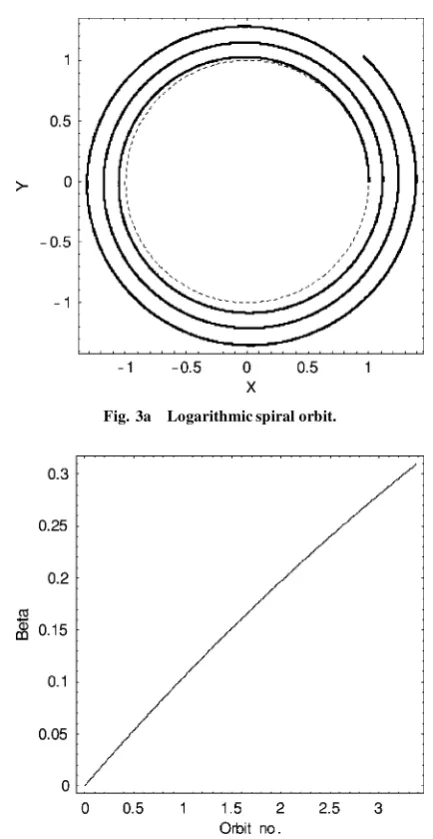
Logarithmic Spiral Orbit

As a further example of the inverse problem, an open logarithmic spiral orbit can be deŽ ned using

r.µ /DrOexp.¸µ/ (20)

for some constant¸Â0; thus, transforming tou.µ /D1=r.µ /and using Eq. (15) yields

¯.µ /D1¡.h2_=¹/u

O.1C¸2/exp.¡¸µ/ (21)

where againuOD1=rO. It can be seen that¯.µ /!1 asµ! 1,

as shown in Fig. 3 (withrOD1), where the orbit number is

de-Ž ned asµ=2¼. In addition, it can be seen that for¯.0/D0, and so

Fig. 3a Logarithmic spiral orbit.

Fig. 3b Required lightness number for a logarithmic spiral orbit.

0·¯.µ /·1, the orbital angular momentumh2_D¹r

O.1C¸2/¡1.

Therefore,the orbitangularmomentumh2_{< ¹r}

Oand so is not equal

to the orbital angular momentum of a circular Keplerian orbit at rDrO. This is also the case for solar sail logarithmic spirals with a

Ž xed, nonradial,sail pitch angle.1_{The constraintdeŽ ned by Eq. (16)}

can now be used to obtain

¸2·uO=u.µ /¡1 (22)

Therefore, ifu.µ /¸uO8µ[r.µ /·rO], then¸2·0 and so such

or-bits are forbidden,whereas ifu.µ /·uO8µ[r.µ /¸rO], then¸2¸0

and so logarithmic spiral orbits exist in this case. It is, therefore, concluded from Eq. (16) that inward spirals are always forbidden whereas outward spirals are allowed.

Last, conservation of angular momentum can be used to obtain the trajectory along the logarithmic spiral orbit. Sincer.µ /2_µP_Dh,

wherer.µ /is deŽ ned by Eq. (20), the timetat polar angleµ(with

µ = 0 attD0) can be obtained by integration as

t.µ /D¡r2

O

¯

2¸h¢[exp.2¸µ/¡1] (23)

so that the trajectory along the logarithmic spiral orbit is deŽ ned as a parametric curve of the form

r.t/DrO

q

1C2h¸t¯r2

O (24a)

µ.t/D.1=2¸/log£1C¡2h¸¯r2

O

¢

746 MCINNES

In addition, note that, because¯.µ /scales as the inverse of the radial distance from the sun, the total radial force acting on the spacecraft scales as the inverse cube of the radial distance from the sun. It is known that an inverse cube force law will generate spiral trajectories.9;11

Doubly Periodic Orbit

In addition to standard families of closed and open orbits, more complex, doubly periodic orbits can also be considered such as

r.µ /DrO[1Cpsin.µ =4/q] (25)

wherepandqare constantsthat parameterizethe orbit.The required lightness number can then be obtained from Eq. (15), as shown in Fig. 4 (withrOD1,pD0.5 andqD4), although it is not listed here

for brevity.

The extremal values of the required lightness number can also be obtained from Eq. (15) by calculating¯0_{.µ /D0, where}

¯0.µ /D ¡.h2_=¹/[u000_{.µ /Cu}0_{.µ /] (26)}

From Eq. (25) it can then be shown that extremal values of¯.µ /

occur whenµD2¼K, for some integerK. The minimum lightness number¯¡_{and maximum lightness number¯}C_{required are then}

Fig. 4a Doubly periodic orbit;p= 0.5 andq= 4.

Fig. 4b Required lightness number for a doubly periodic orbit.

found to be

¯¡D1¡ h2

¹rO

(27a)

¯C_D1¡ h2

¹rO

µ

pq 16.1Cq/2 C

1 1Cq

¶

(27b)

so that ¯¡_{D0 if the initial conditions are representative of a}

Keplerian circular orbit of radiusrO withh2D¹rO. Last, the orbit

period can be obtained from Eq. (11), where the limits of integration for the orbit apsides must be set to [0;4¼/, so that

T D 4 p

¼r2

O

h

»

p

¼C2q0[.1Cp/=2]

0.1Cp=2/ C

q2₀¡1 2Cp

¢

0.1Cp/

¼

(28)

where0is the Euler gamma function. Now that a range of open-and closed-,periodicorbits have been presented by way of example, transfer between circular coplanar orbits will be investigated.

Transfer Orbits

For a spacecraft with a maximum attainable lightness number¯Q, a circular orbit can be sustained over a range of orbit radii, but with a non-Keplerian orbit period. If the initial conditions are represen-tative of a circular orbit of radiusrO, the orbital angular momentum

is given byh2_D¹r

O, as discussed earlier. Therefore, the maximum

orbit radiusrQat which a circular orbit can be sustained is deŽ ned by Eq. (17) as

Q

r DrO=.1¡ Q¯/ (29)

so that the reachable domain for circular orbit transfer isrO·r· Qr

with 0·¯· Q¯. It can be seen that the constraint¯¸0 implies that r¸rO, whereasrQ! 1as¯Q!1. Whereas these circular orbits are

possible over a range of orbit radii, again note that the orbit period will be non-Keplerian, as demonstrated by Eq. (18).

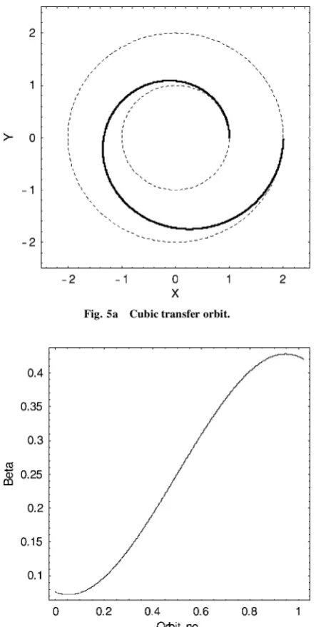
Inverse Transfer Orbit

Because it has been shown that orbits can be deŽ ned a priori, with the constraint 0·¯· Q¯, the problem of transfer between circular orbits can be consideredas an inverse problem. Perhaps the simplest functional form foru.µ /that satisŽ es the boundary conditions for a transfer between circular orbits is the cubic polynomial

u.µ /DuOC3.uf ¡uO/.µ=µf/2¡2.uf ¡uO/.µ =µf/3 (30)

where µf is the transfer angle. Clearly, any choice of orbitu.µ /

that satisŽ es the boundary conditions of the problem must also satisfy Eq. (16). It can be shown thatu.0/DuO andu.µf/Duf,

whereasu0_.0/Du0_.µ

f/D0. The required lightness number can be

determined using the procedure detailed earlier. In addition, the ex-tremal values of the requiredlightnessnumber can be obtained from Eq. (15) by calculating¯0_{.µ /D0. This then results in a quadratic}

equation of the form

µ2¡µµf C2D0 (31)

which yields the polar angles at which the minimum and maximum lightness numbers occurs. When the quadratic is solved, the mini-mum and maximini-mum lightness numbers are found to occur at

µ¡Dµf=2¡

q

µ2

f

¯

4¡2 (32a)

µCDµf=2C

q

µ2f

¯

4¡2 (32b)

Then, substituting forµ¡_andµC_{, and assuming a 360-deg transfer}

numbers, which are found to be

¯¡D¡1 2¡

p

¼2_¡2=2¼Cp_¼2_¡2=¼3¢

£.1¡uf=uO/»0:144.1¡uf=uO/ (33a)

¯CD¡1 2C

p

¼2_¡2=2¼¡p_¼2_¡2=¼3¢

£.1¡uf=uO/»0:856.1¡uf=uO/ (33b)

so that¯¡_{¸0 ifrf ¸rO. Therefore, as with the logarithmic spiral,}

inward transfers are forbidden whereas outward transfers are al-lowed. In addition, asuf !0 (rf! 1/, the maximum required

lightness number is of order 0.856. An example circle-to-circle transfer withµf D2¼is shown in Fig. 5 (withrOD1 andrfD2),

where the extremal values of¯, deŽ ned by Eqs. (33), can be seen.

Elliptical Transfer Orbit

Whereas the use of inverse methods allows the boundary condi-tions for circle-to-circletransferto be satisŽ ed by deŽ ning a transfer orbit apriori, other approaches can also be considered. For exam-ple, an elliptical orbit can be sought that connects the initial and Ž nal circular orbits in a quasiHohmann fashion. For initial and Ž -nal circular orbit radiirOandrf, the required semimajor axis of the

transfer ellipseais.rOCrf/=2. Then, the speedvon the transfer

Fig. 5a Cubic transfer orbit.

Fig. 5b Required lightness number for a cubic transfer orbit.

ellipse at orbit radiusris given by

v2D¹.1¡¯/[2=r¡2=.rOCrf/] (34)

Matching the speed on the transfer ellipse at orbit radiusrO with

the speed on the initial circular orbitp.¹=rO/yields the required

lightness number for the transfer as

¯D 1

2.1¡rO=rf/ (35)

As can be seen from Eq. (17), this is one-halfof the lightnessnumber required to sustain a circular orbit at orbit radiusrf. The transfer

duration¿can also be found from Eq. (11) as one-half of the orbit period of the transfer ellipse so that

¿D¼pa3_{=¹.1¡¯/; aD} 1

2.rOCrf/ (36)

where¯ is deŽ ned by Eq. (35). In summary, the transfer begins with¯D0 at the initial circular orbit of radiusrO. An intermediate

lightness number of.1¡rO=rf/=2 is then required for one-half of

the transferellipse,to transferto the Ž nal circularorbit at radiusrf in

duration¿. Last, the lightnessnumber is increasedto.1¡rO=rf/to

injectthe spacecraftinto the Ž nal circularorbit,with a non-Keplerian orbit period.

Bielliptic Transfer Orbit

An alternative mode of transfer is to construct a transfer com-posed of two ellipses, an initial arc with the maximum lightness number.1¡rO=rf/(as required for a circular orbit at orbit radius

rf/followed by a coast arc. The osculating semimajor axis and

eccentricity at the end of the powered arc must correspond to an apocenter radius on the coast arc equal to the Ž nal circular orbit radius. The length of the initial powered arc must, therefore, be chosen to satisfy this condition. To investigate this requirement, the variational equations for the problem must be formed. Because the effect of the spacecraft thrust is to perturb an osculating two-body ellipse with a radial, inverse square force, the variational equations may be written as1

da dµ D

2ae

1¡e2¯.µ /sinµ (37a)

de

dµ D¯.µ /sinµ (37b)

d!

dµ D ¡

1

e¯.µ /cosµ; e6D0 (37c)

where!is the osculatingargumentof perigee.To proceed,the space-craft will begin on a circular orbit witheD0 andaDaO(aODrO,

the initial circularorbit radius).Then, when Eqs. (37a) and (37b) are integrated over some arc length1µ, with a Ž xed lightness number

¯, the resulting elements are given by

e.1µ /D¯.1¡cos1µ / (38a)

a.1µ /DaO

¯

[1¡¯2.1¡cos1µ /2] (38b)

where Eq. (38b) may be obtained by integrating Eq. (37a), or more easily by using Eq. (38a) in combination with conservation of an-gular momentumh2_D¹a.1¡e2_{/. The osculating apocentre radius}

raDa.1Ce/can then be formed from Eqs. (38) as

ra.1µ /DaO

1C¯.1¡cos1µ /

1¡¯2_{.1¡cos1µ /}2 (39)

Then, whenrpDrf, the condition for orbit transfer becomes

cos2_1µ¡

³

2½¯2_¡¯

½¯2

´

cos1µC

³

1C¯¡½C½¯2

½¯2

´

748 MCINNES

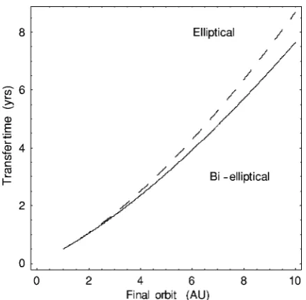
Fig. 6 Transfer duration for elliptic and bielliptic transfer modes.

where½Drf=:rO. The admissible solution to this quadratic is then

found to be

cos1µD1C.1¡½/=½¯ (41)

If Eq. (35) is used to substitute for¯as.1¡rO=rf/=2, it is then

found that1µD¼, as expected. However, if a maximum lightness number of.1¡rO=rf/is substituted, it is found that1µD¼=2.

Therefore, the transfer is composed of two ellipses, each of arc length¼=2.

In summary, the transfer begins with¯D0 at the initial circular orbit of radiusrO. A lightness number of.1¡rO=rf/is then

re-quired for1µD¼=2 to attain the osculating elements required for a coast arc to the Ž nal circular orbit at radiusrf. Last, a lightness

number of.1¡rO=rf/is again required, to inject the spacecraft

into the Ž nal circular orbit. The transfer duration can then be ob-tained by integrating Eq. (11). Although this can be carried out analytically, the full result is not listed here for brevity. A com-parison of the transfer duration for the elliptic and bielliptic trans-fer modes is shown in Fig. 6. Note that in the limitrf !rO it is

found that¿!¼p.r3

O=¹/. This is a limiting process that results

from the formulation of the problem, as can be seen from Eqs. (35) and (36).

Escape Orbits

To reach escape, a switching strategy is required to increase the orbit energy, while the orbit angular momentum is conserved. Be-cause angular momentum is conserved,there will be a curve within thea–eplane along which the transfer to escape will occur. From Eqs. (37a) and (37b), it can be seen that

da de D

2ae

1¡e2 (42)

which integrates toa.1¡e2_/Da

O.1¡e2O/, which is of course a

statement of conservation of angular momentum. The curve in the a–eplane for a spacecraft starting from a circular heliocentric orbit withaOD1 is shown in Fig. 7. As the orbit energy is increased, the

orbit semimajor axis is also increased,leading to an increasein orbit eccentricityuntil escape ateD1. IfeOD0, then, from conservation

of angular momentum, the orbit pericenter and apocenter radii can be obtained as

raDaO=.1¡e/ (43a)

rpDaO=.1Ce/ (43b)

Fig. 7 Curve ina–espace to escape:_², steps along escape ladder with ~

¯= 0.1.

so that in the limitase!1 thepericenterradiusrp!aO=2, whereas

ra! 1. The spacecraft is, therefore, limited to pericenter radii

rpÂaO=2.

It can be seen from Eq. (37a) that a strategy to increase the orbit energy is provided by the following switching law:

¯.µ /D

»

Q

¯ if 0ÁµÁ¼

0 if ¼·µ·2¼ (44)

where¯Qis again the maximum attainable lightness number. Maxi-mum thrust is, therefore, applied on the outward arc, whereas null thrust is required on the inward arc. From Eqs. (38), this results in the following change in orbital elements in thea–eplane

1eD2¯Q (45a)

1aDaO

¯

.1¡4¯Q2/ (45b)

Immediately, it can be seen that escape can be reached on the Ž rst-half orbit if¯QD1

2, since1eD1. If¯QÁ12, then at least one complete

orbit is required before escape can be reached. Similarly, if¯QÂ1 2,

then on the Ž rst arc1eÂ1 and so the orbit semimajor axisaÁ0 as the orbit becomes hyperbolic because the orbit angular momen-tumh2_D¹a.1¡e2_{/is conserved.When Eq. (45) is used, an escape}

ladder can then be formed along the curve of constant angular mo-mentum in thea–eplane such that

ej D2j¯Q (46a)

aj DaO

¯

[1¡.2j¯/Q 2] (46b)

wherejD0¡Mis the number of orbits completed.The steps along the escape ladder from a circular orbit withaOD1 and¯QD0:1 are

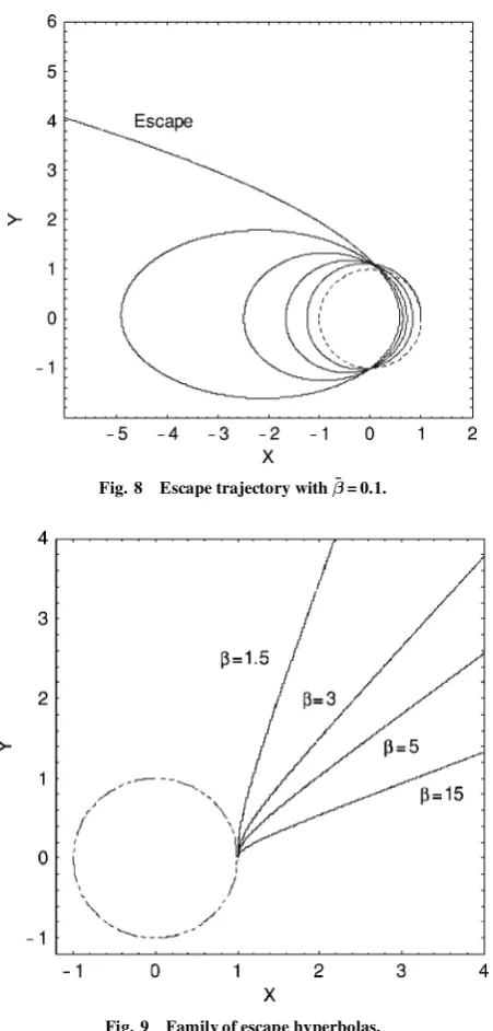
shown in Fig. 7, whereas the resulting escape trajectory is shown in Fig. 8 withrpÂ1₂.

The use of multiple loops for spacecraft with ¯QÁ1

2 can lead

to lengthy escape trajectories. However, future solar sail and M2P2 systems may enable¯QÂ1, which allows direct escape along a hy-perbolic path. Note, however, that the hyperbola does not contain the sun at its focus because the net inverse square force is repulsive. In fact, the sun is located at the center of the two opposing hyper-bolas that deŽ ne the classical conic section. If the initial conditions are representative of a circular of radiusrO, Eq. (10) then provides

the orbit equation as

Fig. 8 Escape trajectory with_¯~_{= 0.1.}

Fig. 9 Family of escape hyperbolas.

so that the orbit has an asymptote at µ1 (asr! 1/ given by

cosµ1D1¡1=¯Q. It can be seen that Eq. (19) is recovered if¯QD1.

In addition, Eq. (11) provides timetas a function of polar angle as

t.µ /D r

3 2

O

p_¹2.¯Q¡1/[1¡ Q¯.1¡cosµ/] tanh

¡1£p_{2¯Q¡1 tan.µ=2/}¤_{C Q¯}p_{2¯Q¡1 sinµ}

.2¯Q¡1/[1¡ Q¯.1¡cosµ/] (48)

Last, equating the energy at the beginning of the orbit arc [v2

O=2¡ ¹.1¡ Q¯/=rO] to the energy asr!(v₁2=2/yields the hyperbolic

excess speedv1as

v1DvO

q

2¯Q¡1 (49)

where vODp.¹=rO/is the speed on the initial circular orbit at

radiusrO. A range of escape hyperbolas are shown in Fig. 9 with

rOD1. It can be seen that a rectilinear orbit, deŽ ned by Eq. (19),

will have an asymptote withµ1D¼=2, whereasµ1!0 as¯! 1. Conclusions

An extension of the classical two-body problem has been inves-tigated that considers the addition of a modulated, radial, inverse square force. The force is assumed to be the modulated thrust from a solar sail or M2P2 system. It has been shown that the forward integration problem can be solved in closed form, whereas an in-verse problem can be constructed that allows orbits to deŽ ned a priori. Both of these approacheshave been used to investigatetrans-fer between circular, coplanar orbits and open escape orbits. For escape orbits, a switching strategy has been deŽ ned that allows mo-tion along an escape ladder in thea–eplane, allowing energy gain, while orbital angular momentum is conserved.

Acknowledgments

Aspects of this work were supported by funding from the Lev-erhulme Trust and the Lockheed Martin Corporation, to whom the author expresses his thanks.

References

1_{McInnes, C. R.,Solar Sailing: Technology, Dynamics and Mission} Ap-plications, Springer-Verlag, London, 1999, pp. 56–111.

2_{Winglee, R. M., Slough, J., Ziemba, T., and Goodson, A.,}

“Mini-Magnetospheric Plasma Propulsion: Tapping the Energy of the Solar Wind for Spacecraft Propulsion,” Journal of Geophysics Research, Vol. 105, No. A9, 2000, pp. 21067–21077.

3_{Zubrin, R., and Andrews, D., “Magnetic Sails and Interplanetary Travel,”} Journal of Spacecraft and Rockets, Vol. 28, No. 2, 1991, pp. 197–203.

4_{Tsien, H. S., “Take-Off from Satellite Orbit,”Journal of the American} Rocket Society, Vol. 23, No. 4, 1953, pp. 233–236.

5_{Battin, R. H.,An Introduction to the Mathematics and Methods of} Astro-dynamics, AIAA Education Series, AIAA, New York, 1987, pp. 408–415.

6_{Modi, V. J., “On the Semi-Passive Attitude Control and Propulsion of}

Space Vehicles Using Solar Radiation Pressure,”Acta Astronautica, Vol. 35, No. 2/3, 1995, pp. 231–246.

7_{Prussing, J. E., and Coverstone-Carroll, V., “Constant Radial Thrust}

Ac-celeration Redux,”Journal of Guidance, Control, and Dynamics, Vol. 21, No. 3, 1998, pp. 516–518.

8_{Akella, M. R., “On the Existence of Almost Periodic Orbits in Low}

Radial Thrust Spacecraft Motion,”Advances in the Astronautical Sciences, Vol. 106, 2000, pp. 41–52.

9_{Broucke, R., “Notes on the Central Force r}N_{,”Astrophysics and Space} Science, Vol. 27, No. 1, 1980, pp. 33–53.

10_{Sweetser, T. H., and Sauer, C. G., “Advanced Propulsion Options}

for Missions to the Kuiper Belt,”Advances in the Astronautical Sciences, Vol. 109, 2001, pp. 2297–2306.

11_{Fowles, G. R.,Analytical Mechanics, Holt-Saunders International, New}