Efficient Fiber Bragg Grating and Fiber Fabry–Pérot
Sensor Multiplexing Scheme Using a Broadband
Pulsed Mode-Locked Laser
Geoffrey A. Cranch, Gordon M. H. Flockhart, and Clay K. Kirkendall,
Member, IEEE
Abstract—A pulsed broadband mode-locked laser (MLL) com-bined with interferometric interrogation is shown to yield an effi-cient means of multiplexing a large number of fiber Bragg grating (FBG) or fiber Fabry–Pérot (FFP) strain sensors with high perfor-mance. System configurations utilizing time division multiplexing (TDM) permit high resolution, accuracy, and bandwidth strain measurements along with high sensor densities. Strain resolu-tions of 23–60nε/Hz1/2at frequencies up to 800 Hz (expandable to 139 kHz) and a differential strain-measurement accuracy of ±1 µε are demonstrated. Interrogation of a low-finesse FFP sensor is also demonstrated, from which a strain resolution of 2 nε/Hz1/2 and strain-measurement accuracy of ±31 nε are achieved. The system has the capability of interrogating well in excess of 50 sensors per fiber depending on crosstalk requirements. A discussion on sensor spacing, bandwidth, dynamic range, and measurement accuracy is also given.
Index Terms—Interferometry, large-scale systems, mode-locked lasers (MLLs), optical fiber transducers, strain measurement.
I. INTRODUCTION
T
HE FIBER Bragg grating (FBG) sensor has been demon-strated as a useful device for measurement of strain, particularly in monitoring the health of structures. It exhibits several advantages over conventional strain-measurement sen-sors based on resistive strain gauges: Many FBGs can be multi-plexed onto a single fiber using techniques described below; the sensor is electrically passive and immune to electromagnetic interference and FBG sensor arrays can be mass produced using automated grating-fabrication techniques. Some high-performance applications of FBG strain sensors require multi-plexing very large numbers of sensors onto a single fiber while achieving submicrostrain resolution from sub-Hertz frequen-cies upwards. High-resolution and dynamic-range strain mea-surement can be achieved with an interferometric wavelength discriminator. This yields strain resolutions approaching the nanostrain level over large bandwidths. Interferometric inter-rogation of FBG strain sensors has demonstrated resolutions of 6 nε/Hz1/2 at 1 Hz for a single sensor [1] and 4 nε/Hz1/2 at 0.1 Hz for a multiplexed array [2]. The latter multiplexingManuscript received April 5, 2005; revised June 10, 2005. This work was supported by the Office of Naval Research.
G. A. Cranch and G. M. H. Flockhart are with SFA Inc., Largo, MD 20774 USA based at the Naval Research Laboratory (NRL), Washington, DC 20375 USA (e-mail: [email protected]; [email protected]).
C. K. Kirkendall is with the Naval Research Laboratory (NRL), Washington, DC 20375 USA (e-mail: [email protected]).
Digital Object Identifier 10.1109/JLT.2005.857735
technique utilizes the spectral selectivity of the FBG sensors to distinguish between them [i.e., wavelength division multiplex-ing (WDM)]. The number of sensors in this case is limited by the spectral width of the emission from the illuminating source and the required wavelength separation and is typically less than 20 sensors. To increase the level of multiplexing, time division multiplexing (TDM) can be applied, where sensors are sequentially arranged such that their signals arrive at the detector at different times. This requires producing switched broadband optical pulses; such as by directly switching a super-luminescent diode (SLD) [3] or by externally modulat-ing an edge LED (ELED) [4] or erbium-doped fiber amplifier (EDFA) [5]. In these cases, strain resolutions of 220 and 2 nε/Hz1/2 were achieved with the SLD and ELED sources, respectively. Sensor count limitations arise in two of these configurations due to the restricted pulse powers generated by SLDs (∼1 mW) and ELEDs (∼100 µW). Higher power is generated with the EDFA source and further increase in power can be achieved with optical amplification; however, this adds to the cost and complexity. Also, multiple-stage optical modu-lators are required to achieve acceptable extinction ratios when operated with a broad-bandwidth input signal. Low extinction ratio pulse emission increases the crosstalk in multiplexed ar-rays and reduces the number of sensors that can be multiplexed. Other noninterferometric techniques to interrogate multiplexed FBGs that have achieved submicrostrain resolution have been demonstrated. One such technique is based on a linear charge-coupled device (CCD) spectrometer [6] and achieves strain resolutions approaching the nanostrain level over bandwidths up to 2 kHz (extendable to 10 kHz) [7], although is currently limited to WDM only. Another technique utilizes an edge filter to convert the change in Bragg wavelength into an intensity modulation. The sensitivity, linearity, and dynamic range of the sensors are thus dependent on the design of the edge filter. However, strain resolutions of 37 and 2 nε/Hz1/2 at
300 Hz have been demonstrated using a pulsed semiconductor optical amplifier (SOA) source and mode-locked laser (MLL), respectively [8]. Finally, an efficient TDM technique has been demonstrated using an SOA in a resonant cavity. The system is capable of interrogating 100 sensors spaced by 20 cm; strain resolutions less than 1µεup to 500 Hz are reported using an edge-filter interrogation system [9].
To achieve the combination of very high multiplexing gain, submicrostrain resolution, low crosstalk, and large band-width (>50 kHz), the present work describes a configuration
combining a broadband mode-locked erbium-doped fiber laser source with interferometric interrogation. The MLL configura-tion can generate broadband (greater than 60 nm) square optical pulses of duration 10–30 ns (tunable by pump power and fiber ring birefringence), and peak pulse powers approaching 1 W, at a repetition rate of several hundred kilohertz [10]. The spectral emission properties of this laser have been investigated further in [11], which demonstrates this laser to be well suited to high-performance interrogation of FBG sensors. The peak power produced by this MLL exceeds that of an SLD and SOA by greater than two orders of magnitude. It is powered by a single pump diode and is therefore more efficient than the externally modulated EDFA source.
In the proposed configuration, a serially multiplexed array of FBG sensors consists of low-reflectivity FBGs, each at a different wavelength. This sequence of FBGs is repeated pe-riodically along a single fiber. A low-cost method of fabricating multiplexed FBG arrays is based on single-pulse grating fabri-cation on the draw tower [12]. Continued development of this technique has considerably improved the quality of the FBGs over the initial demonstrations and may make possible online fabrication of apodized FBGs at predetermined wavelengths. Alternatively, other techniques based on strip and recoat [13] or by writing through the fiber coating [14] are currently available. The proposed configuration is also demonstrated to interrogate fiber Fabry–Pérot (FFP) cavities, which provide greater than an order of magnitude increase in strain sensitivity. These can be fabricated in the same way as multiplexed arrays of FBG sensors.
This paper is arranged as follows. The MLL and multi-plexing scheme are described in Section II. The FBG sensor system performance is presented and analyzed in Section III. Section IV describes the interrogation of a single FFP sensor, using a modified interrogation approach. Finally, a summary is given in Section V.
II. MULTIPLEXINGSCHEME
A. Mode-Locked Laser (MLL)
The MLL comprises a unidirectional ring cavity. The prin-ciple of the passive mode-locking scheme relies on nonlinear polarization switching, where the beat length of the optical fiber within the ring is power dependent, giving rise to a power dependence of the transmission. This yields a stable operating regime consisting of the emission of square-shaped optical pulses. Operation in this so-called multi-beat-length regime results in mode-locked behavior occurring at relatively low pump powers [15]. Stimulated Raman scattering broadens the emitted radiation beyond the erbium window to greater than 60 nm. The MLL characterized here was first reported in [10]. The ring contains a length of erbium-doped fiber, pumped by a 980-nm laser diode, approximately 700 m of dispersion-shifted fiber, a polarizing isolator, and two polarization controllers. The polarization controllers provide the birefringence control required to obtain the mode-locked regime.
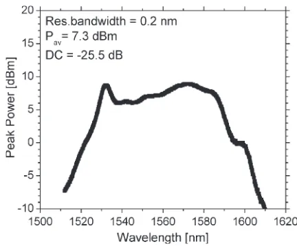
[image:2.594.315.531.66.245.2]Once the mode-locked regime is obtained, the pulsewidth is typically on the order of 10 ns and the repetition frequency frep is 278 kHz (or period of 3.48µs), corresponding to one
Fig. 1. MLL output spectrum.
cavity round-trip time (cavity fiber length 736 m). The optical duty cycle (DC) is therefore 2.8×10⁻³(−25.5 dB). The peak emission power density of the laser is shown in Fig. 1. Thus, the launched pulse power density is 7 dBm at 1550 nm in a 0.2-nm bandwidth. The optical extinction ratio (defined as the ratio of the “ON” to “OFF” power levels) of the MLL is greater than 2222 (33.5 dB). The relative intensity noise (RIN) mea-sured in a 0.23-nm optical bandwidth over the wavelength range 1525–1575 nm is −79 dB/Hz±4 dB at frequencies above 10 kHz and increases to −63 dB/Hz±7 dB at frequencies less than 100 Hz. The error bounds specified here indicate the measured variation with wavelength.
The output emission is polarized with a degree of polariza-tion of ∼ 74%, measured with a Stokes analyzer. The MLL emission is remarkably insensitive to mechanical disturbances of the laser. However, changes in ambient temperature can cause the cavity birefringence to vary and may result in loss of the mode-locked regime. Thus, an environmentally robust system would require the MLL to be thermally isolated or controlled.
To depolarize the emission of the MLL, a Lyot depolarizer (LDPOL or LD) is used. The LDPOL is designed to depolarize the light from the spectrally narrowed reflection of the FBG sensor with a full-width at half-maximum of 0.2 nm. The LDPOL is constructed from two sections of polarization main-taining PANDA fiber (beat length 3.9 mm at 1550 nm) of lengths 102 and 500 m with their fast axes spliced at 45◦ (note that the second section need only be 204 m in length for correct operation). Placing the LDPOL at the output of the MLL reduces the degree of polarization to less than 5%.
B. Interferometric Interrogation Scheme
Fig. 2. Experimental set-up [circulator (CIRC), personal computer (PC)].
the incident radiation, which is a spectral slice over the grating reflection band. Two FBG arrays, each with four FBGs, are thus interrogated simultaneously. The fiber length between each FBG is 91 m. The FBGs are written in single-mode fiber (SMF)-28 fiber and are ∼ 5 mm in length, apodized by the Gaussian laser-beam profile. The FBG’s reflectivities range from 0.8% to 2.1% and have full-width at half-maximum of 0.2 nm. FBGs are numbered 1–4 in FBG array 1 and 5–8 in FBG array 2. The center wavelength of FBGs 1, 2, 5, and 6 is 1549.6 nm and of FBGs 3, 4, 7, and 8 is 1546.6 nm. The signals returning from each array thus consist of a temporal pulse train, where each pulse corresponds to an FBG sensor and consists of a fringe pattern, the phase of which contains the strain informa-tion of interest. The MLL tap is used to generate a trigger pulse for the pulse generator (PG), which generates a pulse train with a controllable delay to trigger the analog-to-digital (A/D) converter. Thus, a single sample is acquired during each pulse return from the FBG array and the signals from all four FBG sensors are recorded by a single A/D. Once digitized, the fringe pattern can be processed to obtain the strain information. The individual FBG sensor signals are extracted during the signal processing. The combined loss of the MZI, circulators, FBG sensor, and connectors results in 6.3µW return power per pulse at the detectors. High-speed (5 MHz) photodiode detectors with integrated transimpedance amplifiers are used for detecting the return from each FBG array. The minimum power required at the detector is approximately 1.6µW per pulse; thus, around 6 dB of optical power margin is available.
The phase-generated-carrier (PGC) interrogation technique is used to extract the interferometric phase, and hence, the Bragg wavelength of the FBG sensor [16]. In this technique, a sinusoidal phase modulation (PM) is applied to one of the arms of the MZI. The processing stages for this method are now briefly described. It is assumed that the split ratios of the directional couplers in the MZI are 50% and there is no excess loss in either interferometer arm. The current generated by the photodetector during a return pulse is then given by
iph=RP(1+V cos [φpgccosωpgct+ ∆φ(t)]) (1)
where R is the photodiode responsivity,P is the peak return power in the absence of the interference term,V is the normal-ized fringe visibility,φpgcis the modulation depth, and∆φ(t)
includes signal and drift phases. Expanding the cosine term in (1) in terms of Bessel coefficients yields
iph=RP+RP V
×
J0(φpgc) +2
∞
k=1
(−1)kJ2k(φpgc) cos2kωpgct
×cos ∆φ(t)−
2 ∞
k=0
(−1)kJ2k+1(φpgc)
×cos
(2k+1)ωpgct
sin ∆φ(t)
.
(2)
Thus, quadrature components of the phase of interest∆φ(t) can be obtained by synchronous detection of the photodiode current at ωpgc and 2ωpgc. Low-pass filtering the resulting
signals yields
RP V J1(φpgc) sin ∆φ(t) (3)
−RP V J2(φpgc) cos ∆φ(t). (4)
The phase is obtained by normalizing the amplitudes of (3) and (4), taking the arctangent of their ratio. Settingφpgcequal
to 2.6 rad results inJ1≈J2; however, a suitable normalization
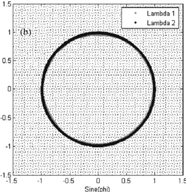
Fig. 3. (a) Three-kilohertz PGC signals and (b) sine/cosine Lissajous plot.
system. This modulation is imparted onto the optical signal in one arm of the MZI with a fiber-wrapped lead zirconate titanate (PZT) tube phase modulator.
A change in wavelength of the FBG causes a change in inter-ferometric phase, given by∆φ=2πndMZI∆λ/λ2FBG, wheren
is the fiber effective refractive index,dMZIis the interferometer
fiber path imbalance, andλFBGis the Bragg wavelength of the
FBG. The fractional change in wavelength with applied strain is given by ∆λ/λFBG=0.78∆ε, where the factor of 0.78
includes the contribution to the Bragg wavelength shift from the stress-optic effect [17]. The phase is thus linearly related to the MZI path imbalance and strain applied to the FBG∆εby
∆φ= 2πndMZI
λFBG
0.78∆ε. (5)
In the experimental system,n=1.468 anddMZI=3.6 ±
0.2 mm, yielding∆φ/∆ε=16.7 mrad/µε.
It is well known that polarization-induced signal fading can occur when a fiber-optic interferometric sensor is illuminated with a polarized light source. However, polarization fading can also occur when an unpolarized light source is used, if the differential or net retardance of the MZI changes. In this case, the normalized fringe visibility in (1) is given by
V = cos
Ωr−s 2
(6)
where Ωr−s is the rotational magnitude of the net-retardance operator of the MZI [18]. An optimum visibility will occur if the net retardance is 0 [i.e.,Ωr−s= 0(modulo 2π)]. Birefrin-gence will generally be present in the MZI and will be different in each arm due to residual birefringence in the optical fiber and any induced birefringence from the phase modulator. During the initial set-up procedure, this birefringence can be (mostly) compensated for by adding a birefringence controller into one arm of the MZI and monitoring the output visibility to obtain an optimum value. Visibilities greater than 0.8 are obtained
in the experimental system. Phase errors due to polarization-dependent loss and birefringence are found to be the primary causes of drift in the FBG sensor system.
III. SYSTEMPERFORMANCE ANDDISCUSSION
The performance of the FBG sensor is primarily determined by the performance of the interrogation system and the fidelity of the signal processing. It is generally of interest to quantify the low-frequency drift of the sensor system, which determines the accuracy of the sensor and the spectral density of the equivalent strain noise when the sensor system is isolated from any external stimulus. This latter characteristic determines the sensor resolution. Different characteristics affect each of these quantities and thus, we shall treat them separately.
dependence of the phase shift in (5), before the differential strain is finally calculated.
A. AC Resolution
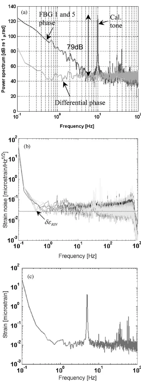
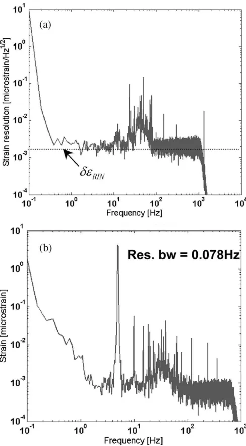
The accuracy of the interferometric phase measurement can be examined by applying a low-frequency PM or calibration tone to the MZI. This tone is common mode to all FBG sensors, and thus, should be canceled when the differential phase is calculated. Fig. 4(a) shows the power spectrum of the interferometric phase when a 10-Hz tone of amplitude∼π rad is applied to the MZI. The differential phase is calculated between FBGs 1 and 5 when they are placed close together. This tone is canceled by 79 dB in the differential phase. Also, note that other low-frequency effects below about 4 Hz are also clearly canceled.
The power spectral density of the strain for all eight sensors is shown in Fig. 4(b). The strain resolution varies between 23 and 60nε/Hz1/2at frequencies below 10 Hz. This corresponds to a phase resolution ranging from 0.38 to 1 mrad/Hz1/2. The data have been filtered above 800 Hz. Fig. 4(c) shows a 4-µε signal at 5 Hz applied to sensor 1.
The strain resolution obtained with this system is poorer than that previously obtained when an erbium fiber amplifier is used as the broadband source [1]. The strain resolution limited by the 0.2-nm linewidth of the FBG reflection is expected to be 0.6 nε/Hz1/2 [19]. The detector noise is also found to
be an order of magnitude less than the measured noise floor. The observed noise floor can be identified as RIN from the MLL. Inspecting (2), it can be seen that RIN will contribute in two ways to the overall photocurrent noise. It will appear in both the first and second terms in (2). In the second term, it effectively becomes an amplitude modulation of the PGC signal. RIN components less thanfpgcwill be common mode
to bothωpgcand 2ωpgccomponents and will be canceled during
the arctangent calculation of (3) and (4). However, white noise components extending above fpgc will contribute an aliased
term to the total RIN. The first term contributes an RIN term to the measured phase since the RIN noise atωpgcis uncorrelated
to the RIN noise at 2ωpgcand does not cancel. The RIN-induced
phase noise due to the first term can be derived using (2) for the case when∆φ(t)1. Substituting(P+δP)forP, whereP is the mean power andδP is the power fluctuation measured in a 1-Hz bandwidth, defining the RIN as RIN= (δP/P)2, and
equating the first term in (2) with the downconvertedωpgcterm
(3) yields this contribution. Finally, adding in the aliased term yields the total noise due to RIN (forJ1J2)
δφRIN
√ 2√RIN 2V J1(φpgc)
. (7)
For the case whenV =0.8,J1=0.33(φpgc=3 rad), and
RIN=−76 dB/Hz at 3 kHz yieldsδφRIN=0.42 mrad/Hz1/2
corresponding toδεRIN=25nε/Hz1/2.
This is marked in Fig. 4(b), and is found to be close to the observed noise levels. Slight variations in the RIN level occur depending on the exact mode-locked state of the MLL, and
[image:5.594.306.553.62.731.2]wavelength [11]. These effects may explain the slight differ-ences in calculated noise floor due to RIN and the measured noise floor.
B. DC Accuracy/Drift
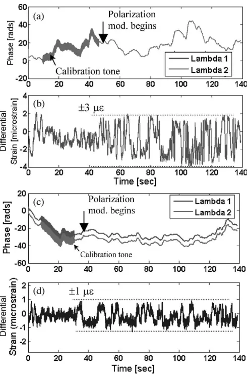
[image:6.594.303.549.66.438.2]The quasi-DC drift of the sensor system can be characterized by measuring the differential strain between two sensors. Fac-tors that will give rise to drift are errors in the interferometric phase measurement and phase errors arising from residual polarization dependences. In the absence of any polarization dependence in the components making up the sensor system, then the sensor output should not be affected by any distur-bance of the connecting leads, even if the source is polarized. However, in practice, there exists net retardance in the MZI, birefringence in the FBG structure and connecting leads, and polarization-dependent loss in the components. In this case, illumination with an unpolarized source will not completely remove sensitivity of the interferometric phase to perturbation of the connecting leads between the MZI and FBG (a similar effect is observed in white-light tandem interferometry [20]). Illumination with a polarized source can, in practice, give rise to very large phase-measurement errors, when birefringence exists in the FBG and MZI and the connecting leads are disturbed. This is demonstrated by removing the LDPOL from the set-up in Fig. 2 and placing a polarization controller between the MZI output and FBG sensor. Changing the birefringence in the connecting leads with the polarization controller during the measurement gives a realistic (although not exactly quantita-tive) indication of phase error due to lead perturbation. This is illustrated in Fig. 5(a), which shows the variation of the interferometric phase for two corresponding FBGs (1 and 5) over time. This plot also shows the calibration procedure. The data are processed in records a few seconds in length. The first record is used to ac couple and normalize the PGC signals, given by (1). A 10-Hz calibration tone is then applied to the MZI, which is used to normalize the sine and cosine signals of (3) and (4) and completes the calibration process. To demon-strate sensitivity of the connecting leads, the birefringence in the connecting leads is changed manually in a random fashion, at the time marked by the arrow. The resulting phase error is clearly visible in the demodulated differential strain shown in Fig. 5(b) (the integration time of this phase measurement is 0.1 s). Changing the birefringence in this way can also affect the transmitted light intensity; however, previous experiments have demonstrated rejection of light intensity fluctuations on the measured phase. During the measurement, the FBGs are placed close together to ensure that any temperature change of the FBG or MZI will be common-mode rejected. The observed drift is thus due primarily to polarization effects with a peak magnitude of±3µε(corresponding to±2.9◦). Fig. 5(c) shows the same measurement when the MLL is depolarized with a Lyot depolarizer [note here that the calibration tone in Fig. 5(a) lasts until∼45 s and in Fig. 5(c) lasts until∼30 s]. The differ-ential strain error, shown in Fig. 5(d), is now reduced to±1µε (peak) (corresponding to±1◦). These levels of phase error were found to be typical for the low-reflectivity FBG sensors. It can be expected that these figures are representative of drift
Fig. 5. (a) Interferometric phase drift for each FBG when connecting lead perturbed (without LDPOL); (b) demodulated differential strain; (c) interferometric phase drift for each FBG when connecting lead perturbed (with LDPOL); (d) demodulated differential strain.
over much longer measurement times due to the mechanism involved.
C. Sensor Bandwidth and Dynamic Range
The sensor bandwidth is determined by the maximum fre-quency signal that can be faithfully reproduced by the signal-processing algorithm. It is related to the PGC frequency or, more specifically, the frequency at which the sine and cosine signals are low-pass filtered. This is usually set to slightly less than the PGC frequency, in this case, 800 Hz. Assuming that the PGC signal has to be oversampled by a factor of 10, then the maximum PGC frequency is 27.8 kHz, thus, the sensor bandwidth can be increased in the present system by an order of magnitude.
The sensor bandwidth can be increased further if a differ-ent interrogation approach is used, such as that based on a 3 ×3 coupler [21]. In this case, the sensor bandwidth is half the interrogation rate, or 139 kHz. This makes possible the use of this system for very-high-frequency strain measurement.
For ac measurements, the dynamic range is also limited by the bandwidth of the signal-processing algorithm. This latter limit has been investigated elsewhere [22]. From signal bandwidth considerations, the maximum peak PM measurable by the interferometric technique isφmax=flpf/fs−1, whereflpfis
the frequency cutoff of the sine/cosine low-pass filter andfsis
the signal frequency. Thus, forfs=10 Hz andflpf =400 Hz,
then φmax=39 rad, which is equivalent to 2335 µε. This
corresponds to a peak wavelength shift of 2.8 nm at 1550 nm. The interferometric measurement of the FBG wavelength is not absolute and is referenced to the phase at the moment of switchON or reset of the signal-processing algorithm. For
measurement of absolute strain, an absolute wavelength mea-surement device is required, such as a CCD spectrometer or wavemeter.
D. Sensor Spatial Separation
The number of sensors that can be multiplexed onto a single fiber can be maximized by combining TDM and WDM. For ex-ample, if the bandwidth allocated to each FBG is 4 nm and the emission bandwidth of the MLL is 60 nm, then the maximum number of wavelengths is 15. The number of sensors that can be time division multiplexed is determined by the return-power requirements and crosstalk considerations. In the present sys-tem, the return power margin is 6 dB; thus, the FBG reflectivity can be reduced by a factor of 4 to∼0.25%. Crosstalk arises from three sources. Multipath-reflection-induced crosstalk oc-curs from the multiple reflections that occur between FBGs of the same wavelength. For a serially multiplexed FBG array, crosstalk signals due to multiple reflections from sensors lead-ing up to sensorncan arrive at the detector at the same time as the primary signal from sensorn. Since the crosstalk signals are incoherent with the primary signal and the FBG reflectivities are low(r1), then only first-order reflections (i.e., signals undergoing three reflections) need to be considered, and the analysis is greatly simplified. Assuming the reflectivities and Bragg wavelengths of the FBGs are identical, then the ratio of the power in the crosstalk signal to the primary signal for the last sensor in an N sensor array (i.e., the worst case) is given by [23]
r2
(1−r2)
(N−2)(N−1)
2 (8)
where r is the FBG power reflectivity. To ensure the strain crosstalk caused by this effect is always less than−40 dB (given by 20log10 of the power ratio), then the maximum number
[image:7.594.308.555.68.248.2]of sensors is 30 for a 0.5% FBG. This increases to 50 for a crosstalk requirement of−30 dB. The source of crosstalk can be reduced by staggering the wavelengths of the FBGs. Leakage light arises from a finite extinction ratio of the optical source (i.e., the light emitted from the source when in its “OFF” state). This will cause light from other sensors to arrive at the detector at the same time as the main pulse. It is straightforward to estimate the magnitude of this effect, since the leakage light will always be incoherent with the pulsed light. By summing
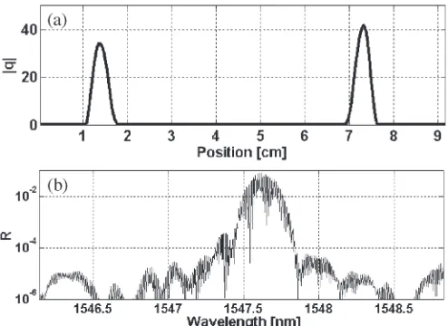
Fig. 6. (a) FFP power reflectivity; (b) FBG coupling coefficient.
the contributions of crosstalk signals from all sensors in the array, the ratio of total crosstalk power due to leakage light to the power in the primary signal is approximated by
ξ−1
N(1+r−rN) 1−2(n−1)r −1
(9)
whereN is the total number of sensors, andξis the extinction ratio of the input signal. Taking the extinction ratio for the MLL to be 33.5 dB andr=0.5%yields a maximum crosstalk level of −36 dB for 30 sensors and −30 dB for 50 sensors. The remaining cause of crosstalk is due to shadowing. This effect can be considered in an ideal array where the FBG reflectivity profiles are ideal Gaussian lineshapes centered at identical wavelengths. A shift in the wavelength of several sensors by the same amount will cause the power transmitted to the subsequent sensors to change (each FBG sees an incident optical spectrum that is a convolution of the source emission spectrum and the previous FBGs spectra). This may give rise to an apparent change in the measured center wavelength or phase of the “shadowed” sensors. This problem is alleviated in a real system if the center wavelengths of the FBGs are not identical and random variations in the reflectivity spectra are present from one FBG to the next.
Assuming a maximum of 50 sensors per TDM and 15 wave-lengths, then the total number of sensors is 750. Increasing the sampling rate to 66 MHz (currently 1.1 MHz) yields a sensor spacing of 20 cm.
IV. INTERROGATION OF ANFFP CAVITY
The proposed multiplexing scheme can also be configured to interrogate low-finesse FFP interferometers. These consist of two closely spaced low-reflectivity FBGs of the same Bragg wavelength. The imbalance in the MZI must be matched to the path imbalance in the FFP, such that the system forms a tandem interferometer arrangement.
with an optical frequency domain reflectometer. The FFP re-places the FBG array in Fig. 2. The power reflectivity of the FFP is shown in Fig. 6(a). An inverse scattering technique is used to obtain the coupling coefficientq of the two FBGs making up the FFP sensor. The amplitude of the coupling coefficient |q|in units of per meter is shown in Fig. 6(b). The two FBGs are Gaussian apodized with a full-width at half-maximum of 3.7 mm, separated by 5.9 cm, and give a peak reflectivity of∼8%.
The current generated by the photodetector during a return pulse (forr1) is given by
iphRP
1+V
2 cos [φpgccosωpgct+φFFP(t)]
(10)
where φFFP(t) is the phase of the FFP cavity (note that this
phase will also include phase shifts generated in the MZI). The amplitude of the interference signal is thus reduced by 0.5 compared with the FBG sensor response.
The imbalance in the MZI is increased to 12.3 cm ±2%, to match the FFP cavity length. For the case when dFFP =
2dMZI, the strain applied ∆ε to the FFP sensor is related to
the measured phase shift by
∆φFFP =
4πndFFP
λFBG
0.78∆ε (11)
where dFFP is the FFP cavity fiber length in the FFP. Ifd=
6.15 cm andλFBG=1547.7 nm, then∆φ/∆ε=0.57 rad/µε.
Thus, the strain responsivity of this sensor is∼33 times larger than that of the FBG sensor. The strain noise of this sensor is shown in Fig. 7(a) and is found to be∼2nε/Hz1/2at
frequen-cies less than 1 kHz (corresponding to a phase resolution of 1.1 mrad/Hz1/2). This represents an improvement in sensitivity of up to 30 times the FBG sensor. The RIN-induced phase noise is given by
δφRIN
√ 2√RIN V J1(φpgc)
. (12)
Using the same values as before yields δφRIN=
0.85 mrad/Hz1/2, corresponding to δεRIN=1.5 nε/Hz1/2,
which agrees well with the measured strain noise. The elevated noise level from 10 to 100 Hz is environmental noise picked up by the FFP sensor. Fig. 7(b) shows a 4-µεtone at 5 Hz applied to the FFP sensor (resolution bandwidth is 0.08 Hz).
[image:8.594.303.547.68.509.2]Birefringence within the FFP cavity and MZI causes polarization-induced phase-measurement errors [20], which lead to strain-measurement errors. To determine the magni-tude of this effect, the MZI and FFP were maintained at a constant temperature and the strain error was measured when the birefringence of the fiber in the connecting lead between the MZI and FFP is changed with a birefringence controller. With a polarized source, the peak magnitude of this strain error is±46nε. Depolarizing the source with the Lyot depolarizer reduces this error to±31nε.
Fig. 7. (a) Strain noise of FFP sensor; (b) 4-µεtone at 5 Hz applied to FFP sensor.
Multiple FFP cavities can be multiplexed in the same way as FBG sensors, providing the cavity lengths of the FFPs are matched to well within the coherence length of the reflected light. Differential strain measurements can also be performed by adding a second set of FFP sensors onto the other output of the MZI.
V. CONCLUSION
temperature. The MLL source is an extremely efficient device for producing pulsed high-extinction broadband radiation and certain configurations are now becoming commercially avail-able. The strain resolutions for an eight-element array vary from 23 to 60 nε/Hz1/2, limited by intensity noise from the MLL. The drift for a differential strain measurement is±1µε when the MLL is depolarized. The sensor bandwidth can be extended to 8 kHz using the current configuration or 139 kHz using an interferometric interrogation based on the 3 × 3 coupler. This system is expandable to over 500 sensors per fiber by combining time division multiplexing (TDM) with wavelength division multiplexing (WDM). Fiber Fabry–Pérot (FFP) sensors can be multiplexed in the same way as FBG sensors. Interrogation of a low-finesse FFP sensor with a 5.9-cm-long cavity yields a strain resolution of 2nε/Hz1/2and
a strain-measurement accuracy of±31nε, which is∼30 times higher than the FBG sensor.
This system provides an efficient means of interrogating very large numbers of closely spaced FBG or FFP sensors. Its high-frequency capability makes it potentially useful for acoustic emission measurement in structures, which requires large numbers of acoustic sensors with submicrostrain resolu-tion. The ability to make differential strain measurements with submicrostrain accuracy makes this system well suited to inter-rogation of multiplexed multicore FBG curvature sensors [24].
ACKNOWLEDGMENT
The authors would like to thank E. J. Friebele for loan of the MLL, C. Askins for his interest and stimulating discussions, and G. Miller for assistance in fabricating the FFP cavity.
REFERENCES
[1] A. D. Kersey, T. A. Berkoff, and W. W. Morey, “Fiber-optic Bragg grat-ing strain sensor with drift-compensated high-resolution interferometric wavelength-shift detection,”Opt. Lett., vol. 18, no. 1, pp. 72–74, 1993. [2] G. A. Johnson, M. D. Todd, B. L. Althouse, and C. C. Chang, “Fiber Bragg
grating interrogation and multiplexing with a 3×3 coupler and a scanning filter,”J. Lightw. Technol., vol. 18, no. 8, pp. 1101–1105, Aug. 2000. [3] Y. J. Rao, A. B. Lobo-Ribeiro, and D. A. Jackson, “Combined
spatial-and time-division-multiplexing scheme for fiber grating sensors with drift-compensated phase-sensitive detection,”Opt. Lett., vol. 20, no. 20, pp. 2149–2151, 1995.
[4] R. S. Weis, A. D. Kersey, and T. A. Berkoff, “A four element fiber grating sensor array with phase-sensitive detection,”IEEE Photon. Technol. Lett., vol. 6, no. 12, pp. 1469–1472, Dec. 1994.
[5] T. A. Berkoff, M. A. Davis, D. G. Bellemore, A. D. Kersey, G. M. Williams, and M. A. Putnam, “Hybrid time and wavelength division multiplexed fiber Bragg grating sensor array,” inProc. SPIE, San Diego, CA, 1995, vol. 2444, pp. 288–294.
[6] C. G. Askins, M. A. Putnam, and E. J. Friebele, “Instrumentation for interrogating many-element fiber Bragg grating arrays,” inProc. SPIE, San Diego, CA, 1995, vol. 2444, pp. 257–266.
[7] C. G. Askins, private communication, Aug. 2004.
[8] D. J. F. Cooper, “Simple high-performance method for large-scale time division multiplexing of fibre Bragg grating sensors,”Meas. Sci. Technol., vol. 14, no. 7, pp. 965–974, 2003.
[9] G. D. Lloyd, L. A. Everall, K. Sugden, and I. Bennion. (2004, Oct.) “Resonant cavity time-division multiplexed fiber Bragg grating sensor in-terrogator,”IEEE Photon. Technol. Lett.[Online].16(10), pp. 2323–2325. Available: www.insensys.com.
[10] M. A. Putnam, M. L. Dennis, I. N. Duling, III, C. G. Askins, and E. J. Friebele, “Broadband square-pulse operation of a passively mode-locked fiber laser for fiber Bragg grating interrogation,”Opt. Lett., vol. 23, no. 2, pp. 138–140, 1998.
[11] G. A. Cranch, C. Kirkendall, “Emission properties of a passively mode-locked fiber laser for time division multiplexing of fiber Bragg grating array applications,” inProc. SPIE, Belgium, May 2005, vol. 5855,17th Int. Conf. Optical Fiber Sensors, pp. 980–983, Paper 5855-241. [12] C. G. Askins, M. A. Putnam, G. M. Williams, and E. J. Friebele,
“Stepped-wavelength optical-fiber Bragg grating arrays fabricated in-line on a draw tower,”Opt. Lett., vol. 19, no. 2, pp. 147–149, 1994.
[13] G. A. Miller, C. G. Askins, P. Skeath, C. C. Wang, and E. J. Friebele, “Fabricating fiber Bragg gratings with tailored spectral properties for strain sensor arrays using post-exposure rescan technique,” inProc. Int. Conf. Optical Fiber Sensors, Portland, OR, May 6–10, 2002, p. 487, Post-deadline paper PD1.
[14] D. S. Starodubov, V. Grubsky, and J. Feinberg, “Efficient Bragg grating fabrication in a fibre through its polymer jacket using near-UV light,”
Electron. Lett., vol. 33, no. 15, pp. 1331–1333, Jul. 1997.
[15] V. J. Matsas, T. P. Newson, and M. N. Zervas, “Self-starting passively mode-locked fibre ring laser exploiting nonlinear polarization switching,”
Opt. Commun., vol. 92, no. 1–3, pp. 61–66, 1992.
[16] A. Dandridge, A. B. Tveten, and T. G. Giallorenzi, “Homodyne demodu-lation scheme for fiber optic sensors using phase generated carrier,”IEEE J. Quantum Electron., vol. QE-18, no. 10, pp. 1647–1653, Oct. 1982. [17] C. D. Butter and G. B. Hocker, “Fiber-optic strain gauge,”Appl. Opt.,
vol. 17, no. 18, pp. 2867–2869, 1978.
[18] A. D. Kersey, M. J. Marrone, and A. Dandridge, “Analysis of input-polarization-induced phase noise in interferometric fiberoptic sensors and its reduction using polarization scrambling,”J. Lightw. Technol., vol. 8, no. 6, pp. 838–845, Jun. 1990.
[19] R. S. Weis and B. L. Bachim, “Source-noise-induced resolution limits of interferometric fibre Bragg grating sensor demodulation systems,”Meas. Sci. Technol., vol. 12, no. 7, pp. 782–785, 2001.
[20] R. R. Gauthier and F. Farahi, “Fiber-optic white-light interferometry: Lead sensitivity considerations,”Opt. Lett., vol. 19, no. 2, pp. 138–140, 1994. [21] M. D. Todd, G. A. Johnson, and C. C. Chang, “Passive, light
intensity-independent interferometric method for fibre Bragg grating interroga-tion,”Electron. Lett., vol. 35, no. 22, pp. 1970–1971, Oct. 1999. [22] G. A. Cranch and P. J. Nash, “Large-scale multiplexing of interferometric
sensors using TDM and DWDM,”J. Lightw. Technol., vol. 19, no. 5, pp. 687–699, May 2001.
[23] W. W. Morey, J. R. Dunphy, and G. Meltz, “Multiplexing fiber Bragg grat-ing sensors,” inProc. SPIE, Boston, MA, 1995, vol. 1586, pp. 216–224. [24] G. M. H. Flockhart, W. N. MacPherson, J. S. Barton, J. D. C. Jones,
L. Zhang, and I. Bennion, “Two-axis bend measurement with Bragg gratings in multicore optical fiber,”Opt. Lett., vol. 28, no. 6, pp. 387–389, Mar. 2003.
Geoffrey A. Cranchreceived the B.Sc. degree in applied physics from the University of Bath, Somerset, U.K., in 1995, and Ph.D. degree in applied physics from Heriot-Watt University, Edinburgh, U.K., in 2001, in the field of fiber-optic sensors and fiber lasers.
He joined GEC-Marconi Naval Systems (now Thales) in 1995 to work on the development of fiber-optic hydrophones and in 1997 moved to the Defence Evaluation and Research Agency, Winfrith, U.K., to continue research on interferometric fiber optic sensor systems and in-fiber Bragg grating (FBG) sensors. Since 2000, he has been employed as a Research Physicist at the Naval Research Laboratory (NRL), Washington, DC. His current research interests are in fiber laser sensors, Bragg gratings, and interferometric sensing techniques.
Dr. Cranch is a Member of the Institute of Physics, U.K., and the Optical Society of America (OSA).
Gordon M. H. Flockhartreceived the M.Phys. degree in optoelectronics and laser engineering and the Ph.D. degree in physics from Heriot-Watt University, Edinburgh, U.K., in 1997 and 2003, respectively.
From 2001 to 2003, he was a Research Associate at Heriot-Watt University, investigating optical FBG-based sensors. In 2003, he joined Virginia Poly-technic Institute and State University, Blacksburg, as a Research Associate under contract from the Naval Research Laboratory (NRL), Washington, DC. Since 2004, he has been a Research Physicist with SFA, Inc., Largo, MD, under contract from the NRL’s Optical Sciences Division. His research interests include low-coherence interferometry, interferometric techniques for interro-gation, multiplexing, and characterization of FBGs, and fiber-optic sensing systems.
Clay K. Kirkendall (S’86–M’86) received the B.S. and M.S. degrees in electrical engineering from George Mason University, Fairfax, VA, in 1987 and 1991, respectively.
![Fig. 2.Experimental set-up [circulator (CIRC), personal computer (PC)].](https://thumb-us.123doks.com/thumbv2/123dok_us/1721840.125584/3.594.147.452.71.252/fig-experimental-set-circulator-circ-personal-computer-pc.webp)