MoL 2018 09: Optimality in Stabilizer Testing

OPTIMALITY IN STABILIZER TESTING

MSc Thesis

(Afstudeerscriptie)

Raja Oktovin Parhasian Damanik

(born October 6th, 1992 in Medan, Indonesia)

under the supervision of Dr Michael Walter, and submitted to the Board of Examiners in partial fulfillment of the requirements for the degree of

MSc in Logic

at theUniversiteit van Amsterdam.

Date of the public defense: Members of the Thesis Committee:

July 9th, 2018 Dr Maris Ozols

Dr Christian Schaffner Dr Michael Walter

Abstract

Stabilizer states are important in quantum information, computation, and error correction. Stabilizer tester is a quantum algorithm that, given an access to several copies a quantum state, tests whether the state is a stabilizer state or far from it. It was an open question whether it is possible to obtain a stabilizer testing algorithm that is efficient and whose power is independent of the number of qubits. The question was answered in [GNW17] which provides a test that is perfectly complete, transversal, and independent of the number of qubits and only requires 6 copies of the state.

Contents

1 Introduction 3

1.1 Motivation . . . 3

1.2 Main contributions . . . 4

1.3 Organization of the thesis . . . 4

2 Preliminaries 6 2.1 Quantum computation and information . . . 6

2.2 Weyl operators . . . 9

2.3 Unitary, Pauli, and Clifford group . . . 10

2.4 Haar measure and quantum statet-design . . . 11

2.5 Representation theory . . . 11

2.6 Stabilizer states . . . 13

2.6.1 Stabilizer formalism . . . 13

2.6.2 Stabilizer states and Lagrangian subspaces . . . 14

2.6.3 Characteristic distribution of stabilizer states . . . 15

3 Stabilizer testing 16 3.1 A 6-copy algorithm . . . 16

3.2 Bell sampling and Weyl measurement . . . 17

3.2.1 Bell sampling . . . 17

3.2.2 Weyl measurement . . . 20

3.3 Brief analysis . . . 21

3.4 Another perspective . . . 24

4.1.1 Quantum state neighborhood bound . . . 29

4.1.2 Application: Neighborhood of stabilizer states. . . 32

4.2 Quantumt-designs and no-go theorem . . . 32

4.3 No-go theorem for 4 copies . . . 34

4.4 Dimension independent stabilizer testing with 5 copies . . . 40

5 Stabilizer testing protocol 42 5.1 A natural stabilizer testing protocol . . . 43

5.2 Bell sampling distribution bound . . . 44

5.3 Stabilizer testing protocols. . . 47

5.3.1 Protocol withk= 1 . . . 47

5.3.2 Perfect-matching protocol . . . 49

5.3.3 Complete protocol . . . 50

5.3.4 Star protocol . . . 52

5.4 Discussion . . . 53

5.4.1 Bell sampling versus Weyl measurement . . . 53

5.4.2 Error Exponent. . . 54

5.4.3 Comparison . . . 58

6 Conclusion and further research 61 6.1 Conclusion . . . 61

6.2 Further research . . . 61

Chapter 1

Introduction

1.1

Motivation

Stabilizer states are quantum states that are useful in measurement based quantum com-putation [RBB03], quantum error correction [Got97], and many other areas in quantum information. Stabilizer states, even though can be produced by relatively simple quantum operation, can be very highly entangled. Entanglement is one of the sources of difficulty in processing quantum mechanical systems using classical computer since the classical de-scription of the state of the quantum objects grows exponentially in terms of the number of qubits. Hence, it might be also hard to learn whether a state is a stabilizer state classically. On the other hand, stabilizer states are the states that can be produced by a class of quan-tum circuit called stabilizer circuit. This quanquan-tum circuit can be simulated efficiently using classical computer [AG04].

It is known that, given an access to copies of an unknown stabilizer state|ψiofnqubits, |ψi can be identified with O(n) copies [AG08]. By identifying, we mean knowing which stabilizer state |ψiis. Also, from an information theoretic argument, at least Ω(n) copies are required [Hol73]. It was an open question whether there exists a stabilizer testing whose parameters do not depend on the number of qubits n [MdW16]. By testing, we mean knowing whether a state |ψiofnqubits is a stabilizer state or far from any of them.

In this thesis, we are interested in studying the optimality of the algorithm in [GNW17] and how to do stabilizer testing optimally with more copies. We are interested to find out whether 6 copies are indeed optimal in a sense that there exists no stabilizer testing algorithm that is independent of the number of qubits which only uses less than 6 copies of the state that we are testing. Moreover, the stabilizer testing algorithm in [GNW17] has perfect completeness but can make type-II error with high probability. To reduce the error, we can design a protocol that repeats the 6-copy algorithm. Such protocol will require 6m

copies where m is the number of repetitions. It was not known whether there is a better protocol for stabilizer testing in terms of the number of copies that is used to reach desirable accuracy and we want to investigate this.

1.2

Main contributions

There are two main contributions of this thesis.

The first contribution is showing that 5 copies are necessary to have a dimension inde-pendent stabilizer testing algorithm. It is known that 6 copies are sufficient [GNW17] for a dimension independent stabilizer testing. Of course, there is a gap, but the proof strategy that we explain might be useful to close this gap. The key idea of the result is to do analysis on average case and relate it to the concept of quantumt-design. More precisely, if randomt

copies of stabilizer states are close a quantumt-design, then the stabilizer testing algorithm satisfying such desired property cannot exist.

The second contribution is an analysis of some protocols that, given access to many copies of the state, can be used to further reduce the error probability of stabilizer testing. A natural protocol for this is an independent and identical repetition of the 6-copy algorithm from [GNW17]. We investigate whether there exists a better protocol to reduce the error than this protocol. We study some protocols that use same primitives as the 6-copy algorithm, namely Bell sampling and Weyl measurements. The answer is affirmative. Aside from that, our analysis gives an insight to how the 6-copy algorithm actually works – we show that one should invest more copies on Bell samplings to obtain better confidence on the stabilizer testing result.

1.3

Organization of the thesis

we should look at this chapter.

Chapter 3 is about stabilizer testing with 6 copies in [GNW17]. We will briefly analyze the algorithm and discuss some of its properties. In the last section, we give some alternative proof to the lemmas and theorems used in the analysis. The technique that we use in the new proof can be used to analyze protocols for stabilizer testing in Chapter 5 later.

Chapter 4 contains one of our main mathematical results, namely the no-go theorem for 4 copies. We will formalize what we mean by no-go theorem for dimension independent stabilizer testing with perfect completeness here. Throughout the chapter we will develop some useful lemmas, such as a lemma about the probability that a random pure quantum state is in the neighborhood of a set of quantum states with respect to trace distance, lemma about quantumt-design and its relation to our no-go theorem, and finally some techniques in representation theory to show that show that random 4-copies of stabilizer states is close to a quantum 4-design.

Chapter 5 contains our other main results, namely about efficiency of protocols for stabilizer testing that can be used to reduce the error. Since the 6-copy algorithm makes a type-II error with high probability in a difficult case, we need to reduce the error. For example, we can use a protocol that repeats the 6-copy algorithm. We show that we can do stabilizer testing in more efficient way in this chapter.

Chapter 2

Preliminaries

In this section, we review briefly some notions from the quantum information formalism that are relevant to this thesis.

2.1

Quantum computation and information

We mainly follow the development of the notions in quantum computation and information from [dW18] and [Wal18].

Given a real or complex matrix

A= 

     

a11 a12 . . . a1n

a21 a22 . . . a2n

..

. ... . .. ...

am1 am2 . . . amn



     

of size m×n, we denote

A†= 

     

a11 a21 . . . am1

a12 a22 . . . am2

..

. ... . .. ...

a1n a2n . . . amn.



If|ui ∈Cd is written in coordinates as

|φi=       u1 u2 . . . ud       ,

we denotehu|=|ui† =u1 u2 . . . ud

. We define

hu|vi=hu| |vi=

d

X

i=1

ui·vi

which will be our standard inner product.

AHilbert spaceHis a real or complex inner product space with norm defined bykuk= p

hu|uifor everyu∈ H. Every quantum mechanical system corresponds to a Hilbert space H. In this thesis, we only finite-dimensional Hilbert space, for example H=Cd for some

positive integerd >1.

A(pure) state of a quantum mechanical systemCd is a unit vector in the spaceCd.

Given two Hilbert spaceH1andH2respectively with inner producth· |·i₁ andh· |·i₂, we

can define a new Hilbert spaceH1⊗ H2whose elements are of the form

X

i

αi·ui1⊗u i 2

where ui

1∈ H1andui2∈ H2for every indexiwith inner producth· |·iis defined by

hu1⊗u2|v1⊗v2i=hu1|v1i1hu2|v2i2

wheneveru1, v1∈ H1 andu2, v2∈ H2. Given two quantum mechanical systemsA andB,

the joint quantum system forA andB isHA⊗ HB.

The simplest quantum mechanical system that we will use isqubit, which is described by two-dimensional Hilbert spaceH=C2. The standard computational basis forC2is denoted

by

|0i:= 1 0

!

|1i:= 0 1

!

which can be seen as the quantum analogue of classical bit 0 and 1, respectively. Some other important states of one qubit are:

|+i=√1 2|0i+

1 √

2|1i, |−i= 1 √

2|0i − 1 √

2|1i, |Li=√1

2|0i+

i

√

2|1i, |Ri= 1 √

2|0i −

i

Together with|0iand |1i, these states are exactly all the stabilizer states of one qubit. A system ofn qubits corresponds to_C2_{⊗. . .⊗}

C2 = (C2)⊗n. A state ofn qubits is a

unit vector |φi ∈ (_C2₎⊗n _{where we use Dirac’s bra-ket notation. Moreover, for n qubits,}

the computational basis is denoted by|x1. . . xni:=|x1i ⊗. . .⊗ |xniwherexi ∈ {0,1} for

i= 1, . . . , n.

Not all vectors in joint systemHA⊗HBis of the form|φi⊗|ψi. Every state that is not in

such tensor product form is called entangled state. For example, Einstein–Podolsky–Rosen (EPR) pair

|Φ00i=

1 √

2(|00i+|11i) is an entangled state inC2⊗C2.

A unitary operatorU is an operator that satisfiesU U†=U†U =I. Transformation of a state|φito another state inHis performed by a unitary operatorU, namely|φi 7→U|φi.

A Hermitian operatorOis an operator that satisfiesO=O†. Every Hermitian operator

Owith the spectral decompositionP

xxPxcorresponds to aprojective measurement {Px}x.

The probability of outcomexwhen we measureO on a state|ψiis tr[Px|ψi hψ|]. After the

measurement,|ψicollapses to

Px|ψi

kPx|ψi k

.

More generally, if{Qx}xis an operator that satisfiesQx≥0 (positive semidefinite) and

P

xQx = I, then {Qx} is called a POVM measurement and each Qx is called a POVM

element.

For a set of pure states {|ψii}i and probability distribution {pi}i, there is a density

operator ρfor this ensemble which is a state of the form ρ=P

ipi|ψi hψ|. For pure states

|ψi, we usually denote|ψi hψ|asψ.

Trace distance between two states ρandσis denoted

T(ρ, σ) := 1

2kρ−σk1= 1 2tr

q

(ρ−σ)†_(ρ−σ)

.

Since density operators ρ andσ are Hermitian, the trace distance can be computed using formula

T(ρ, σ) = 1 2

X

i

|λi|

where λi are eigenvalues of Hermitian matrix ρ−σ. Trace distance is a metric, namely for

all density operatorρ, σ, τ: (i)T(ρ, σ)≥0 with equality iffρ=σ, (ii)T(ρ, σ) +T(σ, τ)≥

Fidelity of two pure states |ϕiand|ψiis given by| hϕ|ψi |2 _{and computes the how close}

the two states ϕand ψ is. For pure states, fidelity is also related to the trace distance as follows:

T(ϕ, ψ) =p1− | hφ|ψi |2_.

2.2

Weyl operators

In one qubit system, the Pauli operators are unitary operators defined by

σ00=I=

1 0 0 1

!

, σ01=X =

0 1 1 0

!

, σ11=Y =

0 −i i 0

!

, σ10=Z=

1 0 0 −1

!

.

Note that each Pauli operator P is a unitary, namely P P† =P†P =I, and a Hermitian, namelyP =P†. Moreover, the Pauli operators that are not identity anti-commute, i.e. they satisfyXY =−Y X,Y Z=−ZY, andZX=−XZ.

In ann-qubit system, for x = (p,q)∈ Zn2 ⊕Z n

2, a Weyl operator Wx =W(p,q) is an

operator of the form

Wx=σp1q1⊗ · · · ⊗σpnqn (2.1) where p= (p1, . . . , pn) and q= (q1, . . . , qn) for some pi, qi ∈ {0,1}. Since Pauli operators

are Hermitian, clearly every Weyl operator is also Hermitian. It is clear that there are 4n

Weyl operators ofnqubits.

We define functionπ:Zn2⊕Z2n 7→Z2as π:x7→p·qfor anyx= (p,q)∈Zn2 ⊕Zn2. We

also define bilinear map [·,·] as

[x,y] =px·qy+py·qx

for anyx= (px,qx) andy= (py,qy).

We can see that for anyx∈Zn2⊕Z n 2,

We also have that for everyx,y∈Zn2 ⊕Z n 2,

WxWy= (−1)[x,y]WyWx. (2.3)

Another useful fact about Weyl operator is that the trace of any Weyl operator ofnqubits must be either 0 or 2n. The later case holds if and only if the Weyl operator is the identity operator.

The scaled Weyl operators

{2−n/2_W

x:x∈Zn2 ⊕Z n 2}

forms an orthonormal basis with respect to the Hilbert-Schmidt inner product hA, Bi = tr[A†B]. Hence, any operatorB on (_C2₎⊗n _{can be written as a linear combination of the}

scaled Weyl operators and we denote cB(x) as the coefficient of 2−n/2Wx of this. We see

that

cB(x) = 2−n/2tr[WxB]. (2.4)

If B is a Hermitian operator (e.g. a pure state B =|ψi hψ|=ψ), cB(x) is a real number.

For any operator AandB, we also have that tr[A†B] =X

x

cA(x)cB(x) (2.5)

If we take AandB as the pure state|ψi hψ|, it follows that

pψ(x) :=cψ(x)2= 2−n| hψ|Wx|ψi |2= 2−ntr[WxψWxψ] (2.6)

is a probability distribution over x∈Zn2⊕Zn2 since by equation 2.5, pψ(x) := cψ(x)2 sum

to 1. We call this thecharacteristic distribution of|ψi. We do not know if this probability distribution has immediate physical interpretation, except via Theorem 3.10.

2.3

Unitary, Pauli, and Clifford group

The set of all unitary operators on _Cd _{forms a group and we call it the unitary groupand}

we denote it byU(d).

In ann-qubit system, thePauli group Pn is defined by,

Pn={±1,±i} × {Wx:x∈Zn2⊕Z n 2}.

TheClifford group Cn of n qubits is a set of unitary operators U on (C2)⊗n such that

U P U† ∈ Pn for all P ∈ Pn. Note that Pn ⊆ Cn. The number of elements of the Clifford

group is

|Cn|= 2n

2_+2n

n

Y

i=1

(4i−1).

For the proof, we refer to [AG04]. Forn >1,Cn is generated by the following operators:

CNOT =      

1 0 0 0 0 1 0 0 0 0 0 1 0 0 1 0

     

, P = 1 0 0 i

!

, and H =√1 2

1 1 1 −1

!

,

acting on arbitrary qubit or pair of qubits. Forn= 1, CNOT gate is omitted.

2.4

Haar measure and quantum state

t

-design

There exists a measuredψon the set of all pure quantum states inCd that satisfies

Z

f(|ψi hψ|)dψ= Z

f(U|ψi hψ|U†)dψ

for all unitary U ∈U(d) and all integrable function f. Indeed, it can be shown that there exists a unique probability measure dψ satisfying such property. We call this measure dψ

theuniform probability measureon the set of pure quantum states, or sometimes also called Haar measure.

A set of quantum states{|ψii}i in Cd is aquantum statet-design if

X

i

(|ψii hψi|)⊗t=

Z

ψ

(|ψi hψ|)⊗t_dψ

where the integral is over the Haar measure. If a set of quantum states forms a quantum

t-design, then it is difficult for a quantum computer to distinguish between the two cases whether it is given a random t copies of a state in such a set or given a random t copies of a pure quantum states. Note that the right hand side is proportional to the orthogonal projection to Symt(Cd) as we will mention later in equation 2.7.

2.5

Representation theory

LetGbe a group with identity element 1. A representation of Gis a Hilbert space H together with a set of unitary operators {Rg : g ∈ G} on H such that for all g, h ∈ G,

RgRh=Rgh. It follows thatR1is an identity onHandRg−1 =R−_g1. In this thesis, we will

mainly use Hilbert space with finite dimension.

Let us study some interesting representations. Let Sn be the set of bijections π :

{1, . . . , n} → {1, . . . , n}. Note that for any d, the Hilbert space (_Cd₎⊗t _{is a}

representa-tion of St where for eachπ∈St, we have a unitary operatorRπ that permutes the tensor

factor

Rπ:|φ1i ⊗. . .⊗ |φti 7→ |φπ−1₍₁₎i ⊗. . .⊗ |φ_π−1_(t)i.

The Hilbert space (_Cd₎⊗t_{is also a representation of the unitary group U(d) where for each}

U ∈U(d), we assign unitary operatorRU

RU :|φ1i ⊗. . .⊗ |φti 7→U|φ1i ⊗. . .⊗U|φti.

We now definesymmetric subspace Symt(_Cd_{) of (}

Cd)⊗tas

Symt(Cd) ={|φi ∈(Cd)⊗t: (∀π∈Sn)Rπ|φi=|φi}.

For a more thorough discussion about symmetric subspace and proofs of some statements below about symmetric subspace, we refer to [Har13].

The dimension of Symt(Cd) is

_t+d−1

n

and

Π(t)_sym= 1

n! X

π∈St

Rπ.

is the orthogonal projector onto Symt(Cd). It is also known that

Z

(|ψi hψ|)⊗tdψ= _t+d

−1

t

−1

Π(t)sym (2.7)

where the integral is over the Haar measure.

Note that Symt(Cd) is a representation for Sn as well as forU(d). This is because for

every π∈St and everyU ∈U(d),Rπ and U⊗t commute. Since the Clifford groupCn is a

subgroup of unitary groupU(2n_{), any representation ofU(2}n_{) is also representation forC} n.

In particular, Symt((C2)⊗n) is also a representation forCn.

Given Hilbert spaceH, a subspaceH1is called aninvariant subspace if for everyg∈G

We say thatHis an irreducible representation if the only invariant subspaces ofH are {0} and Hitself. If H1 ⊆ H is a representation of G, H2 := H1⊥ is also a representation

of G. Then, we can write Has a decomposition of two invariant subspacesH=H1⊕ H2.

This means that every operatorRg can be written as a block diagonal matrix

R1_g 0 0 R2

g

!

where R1g is the restriction ofRg in H1 andR2g is the restriction ofRg in H2.

Anintertwiner J :H1→ H2 is an operator such thatJ Rg1 =R2gJ for allg∈G. If the

intertwiner is invertible, namely

J R1_gJ−1=R2_g,

for allg∈G, then the two representations areequivalent. If there is no such intertwiner, the two representations areinequivalent. IfH1=H2 andR1g=R2g,J is calledself-intertwiner.

Now, any finite representationHcan be decomposed into H=M

i

Hi⊗Cm(i)

where H1, . . . ,Hk correspond to irreducible representations that are pairwise inequivalent

and m(i) is the multiplicity of Hi appearing in the decomposition. Schur’s lemma states

that any self-intertwiner J of suchHis of the form

J=M

i

IHi⊗Mi

where IHi is the identity onHi andMi is an operator onCm(i).

2.6

Stabilizer states

We now review some notions about stabilizer states [Got97]. We mainly follow the develop-ment of the notions related to stabilizer states as in [GNW17].

2.6.1

Stabilizer formalism

A subsetS⊆ Pn isstabilizer group if it is a subgroup of Pauli group which does not contain

−I. Every stabilizer group is Abelian. Note that

PS=

1 |S|

X

P∈S

is a projector onto a subspace that we call the stabilizer code VS associated to S. The

dimension ofVS will be

tr[PS] =

1 |S|

X

P∈S

tr[P] = 2

n

|S|.

If|S|= 2n_{, there will be a unique +1 eigenvector (up to a scalar) of allP ∈S. We call}

such eigenvector of a maximal stabilizer group S a (pure) stabilizer state and we denote it as |Si. The projectorPS will be the one-dimensional projector|Si hS|

As an example, there are 6 stabilizer states of 1 qubits, namely|0i,|1i,|+i,|−i,|Li, and |Ri. There are 30 stabilizer states of 2 qubits. We denote by Stab(n) the set of all stabilizer states ofnqubits. The number of stabilizer states ofnqubits is given by the formula

|Stab(n)|= 2n

n

Y

i=1

(2i+ 1). (2.9)

For the proof, we refer to [AG04]. This fact will be useful later in Chapter 4 to show that the size of the some small neighborhood of stabilizer states with respect to the trace distance is arbitrarily small for largen.

2.6.2

Stabilizer states and Lagrangian subspaces

2⊕Zn2, we denoteN⊥={y∈Z2n⊕Zn2 : (∀x)[x,y] = 0}and dimN

as the dimension ofN. For any subspaceN ofZn2⊕Zn2, we have that dimN+ dimN⊥= 2n.

We call a subspaceN isotropicifN ⊆N⊥ andLagrangian ifN =N⊥. For any isotropic subspaceN of_Zn

2⊕Zn2, we can find a Lagrangian subspace containing

it. If N is a proper subset of N⊥_{, there exists an element a of N}⊥ _{that is not in N.} Define another subspace N1 that contains N as its subspace and a as its element. Since

[a,a] = [a,x] = 0 for allx∈N,N1⊆N1⊥.

IfS is a stabilizer group, we can write

S={(−1)f(x)_W

x:x∈M}

for some subset M ⊆ Zn2 ⊕Zn2 and functionf : M → Z2. In this way, |Si is a (−1)f(x)

eigenvector of Wx. Moreover, if |S| = 2n, M must have size 2n. Moreover, if x,y ∈ M,

thenx+y∈M and sinceS is Abelian, for allx,y∈M, we have [x,y] = 0. Hence,M is a Lagrangian subspace ofZn2⊕Zn2.

Moreover, for any Lagrangian subspace M of _Zn

2 ⊕Zn2, there always exist functions

the stabilizer state corresponding to this stabilizer group. Moreover, other such function f

must be of the form f+δ whereδ(x) = [x,z] for somez∈_Zn

2 ⊕Zn2 and it can be checked

that any function of such form also induces a stabilizer group. For any suchδ, we also have |M, f +δi=Wz|M, fi.

2.6.3

Characteristic distribution of stabilizer states

|Si hS|= 1 2n

X

x∈M

(−1)f(x)_W

x

as in the equation2.8. Hence, by the formula2.4, we have

cS(x) =

 



2−n/2(−1)f(x) _ifx∈M

0 otherwise.

Hence, the characteristic distributionpS(x) for stabilizer state|Si=|M, fiis given by

pS(x) =

 



2−n _ifx∈M,

0 otherwise,

that is a uniform distribution whose support is the set M. Moreover, if|ψi=|M, fiis a stabilizer state, then

ψ=|ψi hψ|=X

x

(−1)π(x)+f(x)_W

x

so |ψiis also a stabilizer state and|ψi=|M, gifor some functiong. Consequently, |ψi=

Chapter 3

Stabilizer testing

We say that a state|ψiofnqubits is ε-far from any stabilizer states if max

S∈Stab(n)

| hS|ψi |2_≤1−ε2_.

We will usually write the expression on the left hand side as maxS| hS|ψi |2. Stabilizer

testing algorithm (orstabilizer tester) is a quantum algorithm that, giventcopies of a state |ψi ∈(_C2₎⊗n_{, accepts if|ψiis a stabilizer state and rejects with non-zero probability if it is}

ε-far from any stabilizer states.

The definition of stabilizer testing algorithm above must depend onεbut in many con-texts of our discussion this is not a problem.

In this chapter, we study a stabilizer testing algorithm from [GNW17] that uses 6 copies of|ψi. In Section 3.1, we write down the algorithm and mention its important properties. In Section 3.2, we discuss some primitives that are used in the algorithm and their properties. In Section 3.3, we give a brief analysis of the algorithm. In Section 3.4, we will look into some parts of the proof and modify them. We show that we can obtain the same analysis without proving the so-called Bell difference sampling theorem. We will use this modification for analyzing stabilizer testing protocol in Chapter 5.

3.1

A 6-copy algorithm

Algorithm 1:Stabilizer testing algorithm with 6 copies.

Input: 6 copies of a state|ψiofnqubits.

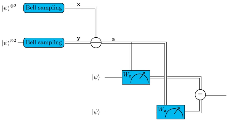
1. Perform Bell sampling twice on two independent copies of|ψi⊗2 each. Let the two sampling outcomes bexandy; each is an element ofZn2 ⊕Z

n 2.

2. Compute the sum (difference)z:=x−y=x+y.

3. Perform WeylWzmeasurement on two independent copies of|ψitwice.

4. Accept iff both WeylWz measurement outcomes agree.

As we will see, the algorithm is perfectly complete, transversal, and independent of the number of qubits. By being perfectly complete, we mean that if the state|ψiis a stabilizer state, the algorithm will accept with probability 1. In this case, the algorithm never makes an error. By being transversal, we mean the algorithm factorizes into qubits of |ψior pair of qubits in |ψi⊗2. This is the nature of Bell sampling and Weyl measurement. By being independent of the number of qubits, we mean that the error of our algorithm does not depend on n. Thus, if we want to reduce the error it does not depend on the number of qubits of our states. This means that the algorithm tests the stabilizerness property of quantum state regardless of the number of qubits.

3.2

Bell sampling and Weyl measurement

3.2.1

Bell sampling

Bell states are useful in the task of quantum teleportation [BBC+_{93] and many other tasks} in quantum information. They are states that are obtained from applying one of the four Pauli operators to one of the two qubits of an EPR pair:

|Φ00i= (σ00⊗I)|Φ00i=

1 √

2|00i+ 1 √

2|11i |Φ01i= (σ01⊗I)|Φ00i=

1 √

2|01i+ 1 √

2|10i |Φ10i= (σ10⊗I)|Φ00i=

1 √

2|00i − 1 √

2|11i |Φ11i= (σ11⊗I)|Φ00i=

1 √

2|01i − 1 √

|ψi⊗2

|ψi⊗2

|ψi

|ψi Bell sampling

Bell sampling

y x

z

Wz

Wz

=

Figure 3.1: A high-level circuit for the 6-copy algorithm. A single line indicates quantum data while double lines indicate that the data is classical. Bell sampling is a primitive that can be performed using CNOT gate, Hadamard gate, and performing measurement in computational basis.

They form an orthonormal basis of (_C2₎⊗2_{. Hence, they correspond to a projective}

mea-surement {|Φxi hΦx|}x∈Z22 on (C

2₎⊗2_.

Now, in the system of 2·nqubits, we denotenEPR pairs as |Φ+_{i= √}1

2n

X

q∈Zn2

|qi ⊗ |qi

where|qi=|q1, . . . , qniis a state in a computational basis corresponding to the components

ofq∈Zn2. We illustrate this in Figure3.2. Forx∈Zn2 ⊕Zn2, applying a Weyl operator Wx

to the firstnqubits, we will obtainnpairs of Bell states, which we denote as |Wxi= (Wx⊗I)|Φ+i.

Projective measurement{|Wxi hWx|}x∈Zn2⊕Zn2 is known asBell sampling [Mon17,ZPDF16].

Moreover, given a state|ψiofnqubits, performing Bell sampling on|ψi⊗2is just performing projective measurement in the Bell basis onncorresponding pairs of qubits from each copy. This means that Bell sampling transversal.

..

. ...

|Φ00i⊗n |Φ+i

Figure 3.2: Two ways of looking at n EPR pairs based on the order of the qubit systems. More precisely, there exists a unitaryJ that permutes the tensor factors such that |Φ+_i=

J|Φ00i⊗ n

.

sampling on|ψi⊗2, namely

tψ(x) =| hWx|(|ψi ⊗ |ψi)|2.

We calltψtheBell sampling distributionof a pure state|ψi. We prove the following formula

fortψ.

Proposition 3.1 (Bell sampling distribution [Mon17]). For any pure state ψ of n qubits, we have that

tψ(x) = 2−n| hψ|Wx|ψi |2.

Proof. The proof uses transpose trick:

tr[|Wxi hWx|ψ⊗2] =hΦ+|(I⊗Wx)ψ⊗2(I⊗Wx)|Φ+i

=hΦ+_|(ψ⊗W

xψWx)|Φ+i=hΦ+|(I⊗WxψWxψ)|Φ+i

= tr[|Φ+i hΦ+|(I⊗WxψWxψ)] = 2−n

X

q

tr[|qi hq|WxψWxψ] = 2−ntr[WxψWxψ],

where the first equation is because trace is cyclic and the definition of |Wxi, the third

equation is by the so called transpose trick and the fact that for pure state ψ,ψ> =ψ, the fourth equation is again because trace is cyclic, and fifth equation is by the definition of |Φ+_{i. It is now easy to see that}

3.2.2

Weyl measurement

Pauli operatorsX,Y, andZ have spectral decompositions as follows:

X =|+i h+| − |−i h−|

Y =|Li hL| − |Ri hR|

Z=|0i h0| − |1i h1|.

So, measuring Pauli operatorsX,Y, andZwill give us an outcome that is their eigenvalues, namely +1 or −1.

For everyx= (p,q)∈_Zn

2⊕Zn2, a Weyl operatorWx onnqubits is just ann-fold tensor

product of Pauli operators

Wx=σp1q1⊗. . .⊗σpnqn.

We defineWeyl measurement as measuring some Weyl operatorWx on a state ofnqubits.

Weyl measurement has two possible outcomes +1 and−1. The projectors that correspond to the outcome +1 and−1 of WeylWx measurement are

I−Wx

2 and

I+Wx

2 ,

respectively. Performing Weyl Wx measurement can also be thought as measuring Pauli

σpiqi to thei-th qubit of|ψi. Hence, together with Bell sampling they perform transversal tests.

If we want to test whether a state|ψiis an eigenvector of a Weyl operator Wx, we can

measure Wx on |ψi several times and accept if and only if all the measurement outcomes

agree. We call this procedureWeyl eigenvector test. Let` be the number of repetitions of the Weyl measurement on ` independent copies of |ψi. Given a state |ψi of nqubits and

x∈Zn2⊕Zn2, we denote bywψ,`(x) the probability that the WeylWx eigenvector test with

` repetitions accepts|ψi. Note thatwψ,`is not a probability distribution overZn2⊕Zn2.

Proposition 3.2. Let|ψibe a state ofnqubits,` >1be a positive integer andx∈Zn2⊕Z n 2.

Then the probability that Weyl Wx eigenvector test with` repetition acceptsWx is given by

wψ,`(x) =

1 +p2n_p ψ(x)

2

!`

+ 1− p

2n_p ψ(x)

2

!`

.

where pψ(x)is the probability distribution in 2.6. Consequently,wψ,`(x) =f`(2npψ(x))for

some polynomial f` with non-negative coefficients. If we fix nas a constant, we also have

Proof. The probability can be computed immediately by computing

tr "

_I+W

x

2 `

ψ⊗2`

# + tr

"

_I−W

x

2 `

ψ⊗2`

#

.

The consequence can be checked by expanding the expression

f`(t) =

_{1 +}√_t 2

` +

₁₋√_t 2

` = 2−`

`

X

i=0

(√t)i+ (−√t)i= 2−` X

0≤i≤`/2

t2i.

In particular, if|ψiis an eigenvector ofWx then cψ(x) = 2−

n

2tr[W_xψ] =±1 and hence

the probability above will be 1. Algorithm1uses Weyl eigenvalue test with`= 2 repetitions. For`= 2, the probability of being accepted by Weyl eigenvector test is

wψ,2(x) =

1 + 2n_p ψ(x)

2 .

3.3

Brief analysis

We begin by showing that Algorithm1has perfect completeness, i.e. accepts stabilizer state with probability 1.

Proposition 3.3 (Perfect completeness of Algorithm1 [GNW17]). If |ψi ∈Stab(n), Algo-rithm1accepts |ψiwith probability1.

Proof. Suppose |ψi is a stabilizer state of n qubits. We can write |ψi =|M, fi for some Lagrangian subspaceM ⊆_Zn

2⊕Zn2 and functionf :Zn2⊕Zn2 →Z2 as mentioned in Section

2.6. There exists z ∈ Zn2 ⊕Zn2 such that |ψi = Wz|ψi. This zdepends on |ψi, which is

unknown. From Proposition3.1, performing Bell sampling on|ψi⊗2will give an outcomex

with probability

tψ(x) = 2−n| hψ|Wx+z|ψi |2=pψ(x+z).

Hence we obtain an xsuch that x+z∈ M but x is not necessarily in M. If we do Bell sampling twice on two independent copies of |ψi⊗2, we will obtain two outcomes x andy

where x+z,y+z∈ M. Note thatx and y are not necessarily in M, but we know that

x+z+y+z=x+ymust be inM sinceM is a subspace. We know that|ψiis a (−1)f(x+y)

eigenvector ofWx+y. Hence,|ψiwill be accepted by eigenvector test corresponding to Weyl

Note that if|ψiis a stabilizer state with real amplitude, namely|ψi=|ψi, we have

tψ(x) = 2−n| hψ|Wx|ψi |2= 2−n| hψ|Wx|ψi |2=pψ(x) (3.4)

so we know the outcome of Bell sampling comes from the setM.

Suppose |ψi is ε-far from any stabilizer states. The idea of the proof is to connect three quantities, namely the probability that the algorithm accepts |ψi, the characteristic distribution pψ, and maxS| hS|ψi |2. In this thesis, we mainly explore some new relations

between the first two quantities and just use the result about the last two quantities. The following lemma shows the relation of the last two quantities.

Lemma 3.5 ([GNW17]). Let |ψibe a pure state ofnqubits. Let M0⊆Zn2⊕Zn2 such that

M0=

x: 2n·pψ(x)>

1 2

. (3.6)

Then,

max

S∈Stab(n)| hS|ψi |

2_≥ X

x∈M0

pψ(x). (3.7)

Proof. We refer the to the proof in [GNW17].

For the analysis of the first two quantities, a new primitive calledBell difference sampling is introduced in [GNW17]. Bell difference sampling is defined as performing Bell sampling twice on two independent copies of the states we are testing and take the difference of the two outcomes. In Algorithm 1, this is the combination of steps 1 and 2.

If|ψi=|M, fiis a stabilizer state, the outcome of Bell difference sampling on four copies of|ψiwill be a samplezfrom and only from the setM, which contains the supports of the characteristic distribution of |ψi. The elements of M correspond to Weyl operators that stabilize|ψi. If|ψiis not a stabilizer state, it is not clear how Bell sampling distributiontψ

is related to the characteristic distribution of |ψi. Let us denote by qψ(a) the probability

of obtaining outcome afrom performing Bell difference sampling on four copies of |ψi. We callqψ theBell difference sampling distribution. Also, the POVM element that corresponds

to outcomea from Bell difference sampling is given by Πa=

X

x

|Wxi hWx| ⊗ |Wx+ai hWx+a|, (3.8)

and the probability is

qψ(a) =

X

x

tψ(x)tψ(x+a). (3.9)

Theorem 3.10 (Bell difference sampling theorem [GNW17]). Let ψ be a pure state of n

qubits. The probability of obtaining an outcome afrom Bell difference sampling is given by

qψ(a) =

X

x

tψ(x)tψ(x+a) =

X

x

pψ(x)pψ(x+a). (3.11)

Proof. We refer to [GNW17] for the proof. We will provide an alternative proof in the next section.

It is not true in general that for anya1, . . . ,am,

X

x

tψ(x)tψ(x+a1). . . tψ(x+am) =

X

x

pψ(x)pψ(x+a1). . . pψ(x+am).

Now, we prove that it rejects non-stabilizer state with non-zero probability.

Proposition 3.12([GNW17]). Let ψbe a state ofnqubits that isε-far from any stabilizer states. Then Algorithm1accepts ψ with probability at most 1−1

4ε 2_.

Proof. We can see that the POVM that corresponds to accepting a state|ψiis given by Πaccept=

X

a

Πa⊗

I⊗2_+W⊗2

x

2 (3.13)

where Πa is a POVM element defined in equation 3.8 corresponding to outcomea of Bell

difference sampling. Then, the probability of accepting|ψiis

paccept= tr[Πacceptψ⊗6] =

1 2

X

a

qψ(a)(1 + 2npψ(a))

= 1 2 X a X x

pψ(x)pψ(x+a)(1 + 2npψ(a)) =

1 2

X

x

pψ(x)(1 + 2n

X

a

pψ(x+a)pψ(a))

≤ 1 2

X

x

pψ(x)(1 + 2n

X

a

pψ(a)2) =

1 2

X

a

pψ(a)(1 + 2npψ(a)),

where the third equation is by Theorem 3.10, the inequality is by the Cauchy Schwarz inequality. By Markov’s inequality, we have

X

a∈M0

pψ(a)≥1−2

X

a

pψ(a)(1−2npψ(a)) = 1−4(1−paccept)

which works because pψ(a) ≤2−n. It follows that if ψ is ε-far from any stabilizer states,

using Lemma 3.7, we obtain 1−ε2≥max

S | hS|ψi |

2_≥ X

a∈M0

pψ(a)≥1−4(1−paccept),

3.4

Another perspective

We prove some facts in the analysis above in a different way. First, we prove Theorem3.10, namely Bell difference sampling theorem, in different way. Second, we also prove

paccept≤

1 2

X

a

pψ(a)(1 + 2npψ(a)).

in a different way; without using the Bell difference sampling theorem. We use the same method later in Chapter 5 to analyze some protocol for stabilizer testing with many copies that is more efficient than just repeating Algorithm 1.

All the propositions below aim to writepψ andtψ in terms ofcψ(x). The behaviour of

the computation is also very similar, namely using Lemma 3.14.

Lemma 3.14. Let x∈Zn2 ⊕Zn2. Then

X

y∈Zn2⊕Zn2

(−1)[x,y]₌

 



2n _{if x= 0,}

0 otherwise.

Proof. Follows from the fact that for anyx∈Zn2 ⊕Zn2, the functionϕ:Zn2⊕Zn2 →Z2

ϕ(y) = (−1)[x,y]

is a homomorphism; and it is a trivial homomorphism if and only ifx=0. We first writepψ andtψ in terms ofpψ.

Proposition 3.15. For any pure state ψof nqubits,

pψ(x) = 2−n

X

y

pψ(y)(−1)[x,y]

tψ(x) = 2−n

X

y

pψ(y)(−1)π(y)+[x,y].

Proof. The first equation can be obtained from the following computation:

pψ(x) = 2−ntr[WxψWxψ] = 2−2n

X

y,z

cψ(y)cψ(z)tr[WxWyWxWz]

= 2−2nX

y,z

cψ(y)cψ(z)(−1)[x,y]tr[WyWz] = 2−n

X

y

cψ(y)2(−1)[x,y].

The second equation can be obtained from the following computation:

tψ(x) = 2−ntr[WxψWxψ] = 2−2n

X

y,z

cψ(y)cψ(z)(−1)π(z)tr[WxWyWxWz]

= 2−2nX

y,z

cψ(y)cψ(z)(−1)π(z)(−1)[x,z]tr[WyWz] = 2−n

X

y

Now, we prove the Bell difference sampling theorem in a different way. Proof of Theorem 3.10. We simply compute

X

x

pψ(x)pψ(x+a) = 2−2n

X

y,z

pψ(y)pψ(z)(−1)[a,z]

X

x

(−1)[x,y+z]=X

y

pψ(y)2(−1)[a,y].

and X

x

tψ(x)tψ(x+a) = 2−2n

X

y,z

pψ(y)pψ(z)(−1)π(y)+π(z)+[a,z]

X

x

(−1)[x,y+z]=X

y

pψ(y)2(−1)[a,y]

where in the last step we use Lemma3.14.

Next, we prove the relation between probability of accepting a state|ψiofnqubits with the characteristic distributionpψ. First we prove the following lemma.

Lemma 3.16. Let ψbe an arbitrary pure state ofn qubits. Then, X

a

tψ(x+a)pψ(a)≤

X

a

pψ(a)2.

Proof. We compute X

a

tψ(x+a)pψ(a) = 2−2n

X

a,y,z

pψ(x)pψ(z)(−1)π(y)+[x,y]+[a,y+z] =

X

y

(−1)π(y)+[x,y]pψ(y)2,

and the inequality immediately follows.

But then some steps in the proof can be slightly changed as follows. Note that our argument does not require the Bell difference sampling theorem.

Alternative proof to Proposition 3.12. We only modify the step of the proof for

paccept=

X

a

qψ(a)(1 + 2npψ(a))≤

X

a

pψ(a)(1 + 2npψ(a)).

To prove this, we observe that X

a

qψ(a)(1 + 2npψ(a)) =

X

a

X

x

tψ(x)tψ(x+a)(1 + 2npψ(a))

=X

x

tψ(x) 1 + 2n

X

a

tψ(x+a)pψ(a)

!

≤X

x

tψ(x) 1 + 2n

X

a

pψ(a)2

!

= 1 + 2nX

a

pψ(a)2

=X

a

Chapter 4

Dimension independent

stabilizer testing no-go theorem

for

t

copies

There are several no-go theorems that are known in theory of quantum computing, such as the quantum no-cloning theorem [WZ82, Die82] or the quantum no-deleting theorem [PB00]. A no-go theorem is usually a mathematical theorem about impossibility of a certain condition to happen.

In this chapter, we will discuss the impossibility of finding a stabilizer tester whose power is independent of the number of qubits with small amount of copies. More precisely, we ask for the minimal number of copies of a state such that we can find a stabilizer testing algorithm that is independent of the number of qubits of the state. It is known that the upper bound is 6 [GNW17]. The main result of this chapter is to show that we have a lower bound of 5. We present this in terms of no-go theorem for 4 copies.

An operator P on Cd is called a (binary) POVM element in Cd if P and I−P is a

positive semi-definite operator on_Cd_.

Definition 4.1(Dimension independent stabilizer testing algorithm with perfect complete-ness for t copies). Let t be a positive integer. A sequence of operators {Π(n)_}

n, where for

each n, Π(n) _{is a binary POVM element on ((}

C2)⊗n)⊗t, is called a stabilizer testing

(i) for any |Si ∈Stab(n), tr[Π(n)(|Si hS|)⊗t_{] = 1, and}

(ii) for any|φi ∈(C2)⊗n that is ε-far from any stabilizer states (ofnqubits),

tr[Π(n)(|φi hφ|)⊗t_]≤f(ε).

The sequence{Π(n)_{}is called dimension independent stabilizer testing algorithm with}

per-fect completeness if there exists such function f that does not depend on n.

In this thesis, we will only discuss stabilizer testing algorithm with perfect completeness, namely the algorithm accepts a stabilizer state with probability 1, as stated in Condition (i). We believe that similar result holds for any stabilizer testing algorithm that can be used for stabilizer testing with high accuracy. The algorithm can only make a type-II error, that is when it accepts a state that is far from any stabilizer states.

Note that if our algorithm has perfect completeness, we can run the algorithm many times to obtain a small error probability. The number of times we repeat the algorithm depends on our knowledge of how often the algorithm accepts a state that is far from any stabilizer states. Condition (ii) from our definition states that we know that the probability of it accepts a state that isε-far from any stabilizer states cannot be larger thanf(ε). Note that if f(ε) gets larger asngets larger, the number of times we need to run the algorithm to obtain a small error probability will be larger as well. Iff(ε) does not depend onn, the number of repetitions is not dependent on nas well. This is good since then we can think that the algorithm really just tests whether a state is a stabilizer state regardless of the number of qubits.

We now define the no-go theorem fort copies.

Definition 4.2 (No go theorem fort copies). The no-go theorem fort copiesis a theorem that states there exists no dimension independent stabilizer testing algorithm with perfect

completeness fort copies.

It is clear that no-go theorem for 6 copies does not hold since we can use{Πn}n from

equation3.13with bound for type-II errorf(ε) = 1−1 4ε

2_{. Our main result in this chapter is}

the no-go theorem for 4 copies. We list the task of investigating whether the no-go theorem for 5 copies as a further research in Chapter 6.

|ϕ1i

|ϕ2i

|ϕ3i

|ϕ4i

ε

Nε(S)

Figure 4.1: Illustration of anε-neighborhood of a set of statesS={|ϕ1i,|ϕ2i,|ϕ3i,|ϕ4i}.

theorem for 4 copies. We describe a strategy to prove the no-go theorem for 5 copies in Section 4.4.

4.1

Neighborhood of quantum states

4.1.1

Quantum state neighborhood bound

Definition 4.3 (ε-neighborhood of a state). Let |ϕi ∈(_C2₎⊗n _{be a pure state of n qubits.}

We define the ε-neighborhood of|ϕias

Nε(ϕ) ={|ψi ∈(C2)⊗n :| hϕ|ψi |2≥1−ε2}.

Then, by definition, we have that Nε(|ϕi) ={|ψi ∈(C2)⊗n : T(|ϕi,|ψi)≤ε} is a ball

centered at |ϕi of radiusε, where T is a trace distance. The complement Nε(|ϕi)C is the

set of all states ofnqubits that areε-far from|ϕi.

It is natural to define what we mean by anε-neighborhood of a set of states is. If we are given a set of states, instead of only one state, it is natural to call a state close to such a set if it is close to some state in the set. Figure 4.1is an illustration for anε-neighborhood for a set of states.

of nqubits. We define the ε-neighborhood ofS as

Nε(S) =

[

ϕ∈S

Nε(ϕ).

Suppose we are given a state|ϕiand a real numberε >0. Asεgoes to 0, there should be less and less states in the ε-neighborhoodNε(ϕ) of|ϕi. We want a quantitative version

of this via the notion of probability. We can ask the following similar question: If we pick a state|ψirandomly according to the Haar-measure, what is the probability that it lies in the neighborhood of |ϕi? The main result of this section is the following theorem which gives us an upper bound of picking a state that is in anε-neighborhood of|ϕi.

Theorem 4.5 (State neighborhood bound). Let ε >0 be a real number such that ε2_< 1 2

and|ϕi ∈(_C2₎⊗n _{be a pure state of n qubits. Then, the probability of a Haar random pure}

stateψ∈(C2)⊗n is inNε(ϕ)can be bounded as follows:

Pψ[ψ∈Nε(ϕ)]≤ 2e·ε2

2n−1

.

We first prove some lemmas.

Lemma 4.6. Let ε∈(0,1), then the inequality (1−ε2)ε12−1≥ 1

e

holds. Consequently, if` is the largest integer such that`≤ 1

ε2, then(1−ε

2₎`−1_≥ 1 e.

Proof. Forε∈(0,1), we have that _ε12 −1>0 and hence

0< 1

(1−ε2_)ε12−1

=

1 + ₁ 1

ε2 −1

_ε12−1

≤e

where we use the inequality (1+1/x)x_{≤eforx >0, and hence it follows that (1−ε}2_)ε12−1_≥

1

e. Now, the second statement follows since if`≤ 1

ε2, we have

(1−ε2)`−1≥(1−ε2)ε12−1_≥ 1

e.

Lemma 4.7. Let |φi ∈(C2)⊗n∼=C2

n . Then

Eψ[| hφ|ψi |2t] =

₂n_+t−1

t

−1

Proof. Note that

Eψ[| hφ|ψi |2t] =Eψ[hφ|

⊗t

|ψi⊗thψ|⊗t|φi⊗t] =hφ|⊗t_Eψ[|ψi

⊗t

hψ|⊗t]|φi⊗t =hφ|⊗t

Z

|ψi⊗thψ|⊗tdψ

|φi⊗t =hφ|⊗t

2n+t−1

t

−1

Π(t)_sym|φi⊗t =

2n+t−1

t

−1

hφ|⊗t|φi⊗t =

₂n_+t−1

t

−1

,

where the second last equality follows from the fact that |φi⊗t∈Symt((C2)⊗n).

We are now ready to prove our main theorem in this section. Proof of Theorem 4.5. By Markov’s inequality, we have

P[ψ∈Nε(ϕ)] =P[| hϕ|ψi |2≥1−ε2]≤ E[| h

ϕ|ψi |2t_]

(1−ε2₎t ,

for an arbitraryt >0. We can upper boundE[| hϕ|ψi |2t] for any positive integertas follows: E[| hφ|ψi |2t] =

_{t+ 2}n₋₁

t

−1

=

2n₋₁ Y

k=1

k t+k ≤

₂n₋₁

t+ 2n₋₁

2n−1

,

where the first equality is by Lemma4.7, the second equality is by definition of binomials, and the last inequality follows from the fact that for t > 0, the function f(x) = _t+xx is increasing.

Now, if we take t= (2n−1)(`−1) where ` is the largest integer less than or equal to 1/ε2 _{we have}

P[ψ∈Nε(ϕ)]≤

1 (1−ε2₎t

₂n₋₁

t+ 2n₋₁

2n−1

= 1

(1−ε2₎(`−1)(2n₋₁₎ 1

`2n₋₁ ≤ e

`

2n−1

,

where in the last inequality, we use Lemma 4.6. Now, ifε2 _< 1

2, then since` is the largest

integer that is less than or equal to 1/ε2_,

P[ψ∈Nε(ϕ)]≤

e

`

2n−1 ≤

e

1 ε2 −1

2n−1

≤ 2e·ε22

n₋₁

We can also bound the probability of picking a state |ψi over Haar-measure that falls into theε-neighborhood of a setS that is finite.

Corollary 4.8. Let ε >0 be a real number such thatε2 _< 1

2 andS be a finite set of pure

states of n qubits. Then the probability that a Haar random pure state |ψi ∈(C2)⊗n is in

Nε(S)can be bounded as follows:

P[ψ∈Nε(S)]≤ |S|· 2e·ε2

2n−1

.

Proof. By the union bound,

P[ψ∈Nε(S)]≤

X

ϕ∈S

P[ψ∈Nε(ϕ)]≤ |S|· 2e·ε2 2n−1

.

4.1.2

Application: Neighborhood of stabilizer states

We discuss an application of the state neighborhood bound in case of S being the set of stabilizer states of n qubits. We will use this fact as an ingredient to prove some no-go theorems for stabilizer testing later.

Lemma 4.9. There existsε0>0 such that

lim

n→∞P[ψ∈Nε0(Stab(n))] = 0. Proof. Recall that

|Stab(n)|= 2n

n

Y

i=1

(2i+ 1)≤2n

n

Y

i=1

2i+1≤212(n 2_+5n)

.

Let us take ε0=

p

1/12, then by Corollary4.8,

P[|ψi ∈Nε0(Stab(n))]≤2 1 2(n

2_+5n)e 6

2n−1 ≤212(n

2_+5n)

2−2n+1.

Hence, asngoes to infinity, the probability goes to 0.

4.2

Quantum

t

-designs and no-go theorem

For positive integers n and t, let us denote by %n,t the uniform average of the t-th tensor

power of states in (C2)⊗n. More precisely,

%n,t=

Z

where the integration is over the Haar measure. Similarly, we denote by σn,t the uniform

average of thet-th tensor power of states in Stab(n), the set of stabilizer states ofnqubits. More precisely,

σn,t=

1 |Stab(n)|

X

|Si∈Stab(n)

(|Si hS|)⊗t_.

It is known that stabilizer states form a quantumt-design fort= 2 andt= 3 [KG15]. We show that the fact that stabilizer states constitute a uniformt-design implies a no-go theorem fort copies.

Theorem 4.10 (No-go theorem for 3 copies). There exists no dimension independent sta-bilizer testing algorithm with perfect completeness given3 copies.

Proof. Suppose, for the sake of contradiction, there exists a dimension independent stabilizer testing algorithm{Π(n)_}

n. From the first condition (i), we know that tr[Π(n)σn,t] = 1. But

then since σn,t =%n,t, we deduce tr[Π(n)%n,t] = 1. But note that for anyε, by linearity of

trace,

tr[Π(n)%n,t] =

Z

Nε(Stab(n))

tr[Π(n)(|ψi hψ|)⊗t_]dψ+

Z

Nε(Stab(n))C

tr[Π(n)(|ψi hψ|)⊗t_]dψ

Note that

Z

Nε(Stab(n))

tr[Π(n)(|ψi hψ|)⊗t_]dψ≤

Z

Nε(Stab(n))

dψ=p(n)_ε

where p(n)ε =P[ψ∈Nε(Stab(n))]. Moreover, by condition (ii) for Π(n), we have that

Z

Nε(Stab(n))C

tr[Π(n)(|ψi hψ|)⊗t_]dψ≤

Z

Nε(Stab(n))C

f(ε)dψ=f(ε)(1−p(n)_ε ).

It follows that for all positive integernand allε >0, we have

1≤p(n)_ε +f(ε)(1−p(n)_ε ) =p(n)_ε (1−f(ε)) +f(ε).

By Lemma4.9, there existsε0>0 such that limp (n)

ε0 = 0 fornlarge and thus we must have

f(ε0) = 1, which is a contradiction.

In the proof above, we use the fact thatσn,3=%n,3. We show that ifσn,tis asymptotically

close to%n,t asn goes to infinity with respect to the trace distance, then a no-go theorem

Theorem 4.11 (Being asymptotically close tot-design implies no-go theorem fortcopies).

Let t be a positive integer such that lim

n→∞kσn,t−%n,tk1= 0.

Then, there exists no dimension independent stabilizer testing algorithm with perfect

com-pleteness fort copies.

Proof. Supposetsatisfies the condition above. Let us denote

δ(n) = tr[Π(n)σn,t]−tr[Π(n)%(n,t)].

Recall that for tr[Π(n)_σ

n,t]−tr[Π(n)%n,t]≤ 1₂kσn,t−%n,tk1for alln, and by the condition in

the theorem, we have

lim

n→∞δ(n) = 0.

By similar reasoning as in Theorem 4.10, we have that for everyε >0 and every positive integer n,

1−δ(n) = tr[Π(n)%n,t]≤p(n)ε (1−f(ε)) +f(ε).

Now since limn→∞δ(n) = 0, together with Lemma 4.9, there exists ε0 > 0 such that

f(ε0) = 0, a contradiction.

4.3

No-go theorem for

4

copies

In this section, we prove the no-go theorem for 4 copies1. According to Theorem 4.11, it suffices to prove that

lim

n→∞kσn,4−%n,4k1= 0.

There is a formula to compute σn,4 in [ZKGG16] andσn,t for anyt in [GNW17]. We will

use results from [GNW17] since its most general result might be applicable to the no-go theorem for 5 copies as we will discuss briefly in Section 4.4.

To every subspaceT ⊆Zt2⊕Zt2, we consider an operatorr(T) on (C2)⊗tdefined by

r(T) = X

(x,y)∈T

|xi hy|

where |xi=|x1, . . . , xti is a computational basis vector corresponding to x∈Zt2. We can

also define an operatorR(T) on ((_C2₎⊗t₎⊗n _{byR(T) =r(T)}⊗n_.

We define a bilinear formβ :_Zt

2⊕Zt2×Z2t⊕Zt2→Z2defined by

β((x,y),(x0,y0)) =x·x0+y·y0

for all (x,y),(x0,y0)∈_Zt

2⊕Zt2. A subspaceT ⊆Zt2⊕Zt2 is calledLagrangian subspace with

respect toβ if for all (x,y),(x0,y0),β((x,y),(x0,y0)) = 0 and dim(T) =t. We define Σt,tas

the set of Lagrangian subspaces ofT ⊆Zt2⊕Zt2with respect to bilinear formβ which also

satisfy the following condition: for all (x,y)∈T:

t

X

i=1

xi≡ t

X

i=1

yi (mod 4),

where xi andyi are the representatives in{0,1} of the components ofx andy. We define

∆ ={(x,x) :x∈Zt2}. We have ∆∈Σt,tandR(∆) =I. The number of elements of Σt,t is

given by

|Σt,t|= t−2

Y

i=0

(2i+ 1). (4.12)

We refer to [GNW17] for the proof. ForT ∈Σt,t,R(T) are the basis of the commutants of

t-th tensor power of the Clifford groupCn which is the main result of [GNW17].

With symmetry, we can understand the structure of Σt,t better. We define a natural

symmetry group for Σt,t. An operator O of Zt2 is called orthogonal if it satisfies OO> =

O>O =I. DefineOtto be the set of orthogonal operatorsO onZt2 which also satisfy the

following condition: for allx,y∈Zt2such thatx=Oy, t

X

i=1

xi≡ t

X

i=1

yi (mod 4).

Ot forms a group. It is easy to see that the permutation groupSt ⊆Ot for all t. Indeed,

for t ≤ 5, St = Ot. Interestingly, O6 has more elements than S6, since S6 contains the

anti-identity operator

A1=

          

0 1 1 1 1 1 1 0 1 1 1 1 1 1 0 1 1 1 1 1 1 0 1 1 1 1 1 1 0 1 1 1 1 1 1 0

Next, we define the action of O ∈ Ot on elements of Σt,t. It has left action and right

action. The left action ofO on T is defined as follows:

OT ={(Ox,y) : (x,y)∈T}.

Similarly, theright action of O on T is defined as

T O={(x, O>y) : (x,y)∈T}.

The action makes sense since for all O ∈ Ot and T ∈ Σt,t, OT and T O are both in Σt,t

again. In addition, the operatorsR(T) also behave nicely. When T ∈Σt,t andO, O0 ∈Ot,

we have that

R(O)R(T)R(O0) =R(OT O0),

where

R(O) :=R(O∆) = X

x

|Oxi hx| !⊗n

.

Now, Σt,t can be decomposed into disjoint cosets with respect to the left and the right

action ofOt:

Σt,t= k

[

i=1

OtT(i)Ot

for someT(i)_{in Σ}

t,tthat has different orbits with respect to left and right action ofOt. We

can always chooseT(1)= ∆ and note that the orbitOt∆Ot=Ot∆.

With this decomposition, for smallt, we can understand the operatorsR(T) forT ∈Σt,t

in a way that it is useful for our computation ofσn,t. The formula forσn,t is given by:

σn,t =

1

Nt

X

T∈Σt,t

R(T) (4.13)

where

Nt= 2n t−2

Y

i=0

(2n+ 2i),

where the equality in equation 4.13 is up to permutation of tensor factors ((_C2₎⊗t₎⊗n ∼₌

Consider the following subspace ofZ42⊕Z 4 2

T4=

     

1 1 0 0 1 1 0 0 1 0 1 0 1 0 1 0 1 1 1 1 0 0 0 0 0 0 0 0 1 1 1 1

      (4.14)

where the rows are the basis ofT4and each row represents a basis element (x,y) wherexis

on the left of the middle line andyis on the right of the middle line. Every element ofT4 is

of the form and only of the form (x,x) or (x,x) wherex1+x2+x3+x4≡0 (mod 2). Here,

forx∈Z42,xdenotes the string Z42with all the bits flipped. For example, 1010 = 0101.

It is easy to show thatπT4 =T4πfor all π∈ S4, and hence R(T4) commutes with all

operatorsR(π). Moreover,R(T4) is proportional to a projector operator.

Lemma 4.15. R(T4)2= 2n·R(T4).

Proof. SinceR(T4) =r(T4)⊗n, it suffices to show thatr(T4)2= 2·r(T4). LetE⊆Z42be the

set of allx∈Z42such thatx1+x2+x3+x4≡0 (mod 2). We can write

r(T4) =

X

x∈E

|xi hx|+X

x∈E

|xi hx|,

and hence

r(T4)2=

X

x,y∈E

|xi hx|yi hy|+ X

x,y∈E

|xi hx|yi hy|+ X

x,y∈E

|xi hx|yi hy|+ X

x,y∈E

|xi hx|yi hy|

= X

x∈E

|xi hx|+X

x∈E

|xi hx|+X

x∈E

|xi hx|+X

x∈E

|xi hx|

= 2·r(T4),

as desired.

Observe thatR(T4)2= 2n·R(T4). There are exactly 4 elements ofSn that stabilizesT4

and they are the Klein-four group K4⊆S4, namelyK4={id,(12)(34),(13)(24),(14)(23)}.

The orbit of T4 with respect to the left and right action of Ot is given by πT4 for π ∈

{id,(12),(13),(14),(123),(132)} giving in total 6 elements inS4T4S4. Together with S4∆

which has size 24, this gives the whole Σ4,4=S4∆∪S4T4S4which has size 30 from equation

4.12.

The set of the commutants of the 4-th tensor power of the Clifford group in ((_C2₎⊗n₎⊗4

is spanned by

Restricted to Sym4((C2)⊗n), the commutants are spanned by only two operators, namely

ISym4_((C2₎⊗n₎ andI_Sym4_((C2₎⊗n₎R(T4)Sym4_((C2₎⊗n₎. Suppose Sym4((_C2₎⊗n_{) can be decomposed as}

Sym4((C2)⊗n) =

M

i

Hi⊗Cmi

where theHi’s are inequivalent irreducible representations of the Clifford groupCn andmi

are the multiplicities of Hi. By Schur’s lemma, the dimension of the intertwiner is given

by the formula P

im 2

i. Since the dimension of the commutants of 4-th tensor power of

the Clifford groupCn in Sym4((C2)⊗n) is 2, it follows that Sym4((C2)⊗n) decomposes into

two inequivalent irreducible representations Sym4((C2)⊗n) = H1⊕ H2 with respect to the

Clifford groupCn.

LetP1 andP2 be the projections ontoH1 andH2, respectively. Note that

%n,4=βISym4_((C2₎⊗n₎=βP1+βP2

where

β−1= dim(Sym4((_C2)⊗n)) = (2

n_{+ 3)(2}n_{+ 2)(2}n_{+ 1)2}n

24 . (4.16)

Note thatP12=P1, P22=P2, andP1P2=P2P1= 0.

Using formula4.13, we also have

σn,4=β1P1+β2P2

for some β1, β2. Then for every positive integerk,

σn,4k =β1kP1+β2kP2. (4.17)

We will compute β1 and β2 as follows. According the formula 4.13, we know that

σn,4= (A+B)/N4 where

A= X

π∈S4

R(π) (4.18)

B= X

T∈S4T4S4

R(T). (4.19)

We prove the following facts about operatorsAandB.

Lemma 4.20. Let A and B be operators that are defined in equation 4.18 and equation

(i) A2= 24·A,

(ii) A·B=B·A= 24·B, and (iii) B2_{= 6·2}n_·B.

Proof. (i) Note that for allπ∈S4,R(π)A=A soA2= 24A. (ii) Note that for all π∈S4,

R(π)B = BR(π) = B so A·B = B·A = 24·B. (iii) Note that R(T4)2 = 2n·R(T4) by

Lemma 4.15and that R(π)R(T4) =R(T4)R(π) for allπ ∈S4. Hence,B2 = 6·2n·B since

for

This way, (A+B)k_=a

kA+bkBfor some{ak}and{bk}. It is easy to prove by induction

that the sequence{ak} and{bk}satisfy

ak+1= 24ak

bk+1= 24ak+ (24 + 6·2n)bk

witha1=b1= 1. It is also easy to see by induction that{ak}and{bk}have closed formulas

ak = 24k−1

bk =

(24 + 6·2n₎k₋₂₄k

6·2n .

Rearranging the term, we obtain

σ_n,4k = 24

k

Nk 4

A+(24 + 6·2

n₎k₋₂₄k

Nk 4·6·2n

B = 24 N4 k A 24− B

6·2n

+

24 + 6·2n

N4

k

B

6·2n.

Letting

P1=

A

24 −

B

6·2n andP2=

B

6·2n,

it is easy to verify thatP1andP2are orthogonal projectors. Comparing with equation4.17,

we find

β1=

24

2n₍₂n_{+ 1)(2}n_{+ 2)(2}n_{+ 4)} andβ2=

6

2n₍₂n_{+ 1)(2}n_{+ 2)}, (4.21)

where the indices are just assigned arbitrarily.

Next, we denoted1= dim(H1) andd2= dim(H2), we can solve the following system

β1d1+β2d2= tr[σn,4] = 1

d1+d2= dim(Sym4((C2)⊗n) =

₂n_{+ 3}

4

to obtain

d1=

(2n_{+ 4)(2}n_{+ 2)(2}n_{+ 1)(2}n₋₁₎

24 ,

d2=

(2n_{+ 2)(2}n_{+ 1)}

6 .

Theorem 4.22 (σn,4 is asymptotically close to a 4-design). limn→∞kσn,4−%n,4k1= 0.

Proof. We compute using coefficients that we find in equation 4.16and equation4.21. We see that

kσn,4−%n,4k1=k(β1−β−1)P1+ (β2−β−1)P2k1

=|β1−β−1|d1+|β2−β−1|d2

= 2

1 2n −

4 2n₍₂n_{+ 3)}

≤2· 1 2n = 2

−n+1_,

and hence the limit is 0 asngets larger.

Hence, we have proved a no-go theorem fort= 4 copies.

Corollary 4.23 (No-go theorem for 4 copies). There exists no dimension independent sta-bilizer testing algorithm with perfect completeness for4 copies.

4.4

Dimension independent stabilizer testing with

5

copies

We have not found a no-go theorem for 5 copies nor a stabilizer testing algorithm that only use 5 copies of the state. But if one believes that no-go theorem for 5 copies hold, one can try to work with the same proof strategy as before in proving the no-go theorem for 4 copies with the same goal, namely to show that average 5 copies is close to a quantum 5-design with some techniques from representation theory.

There are some similar results that we found in the case of 4 copies and 5 copies. For example, we know that the group of orthogonal operatorsO5 in Z52coincides Moreover, we

can decompose Σ5,5 into two cosets with respect to the left and right action ofO5, namely

where

T5=



       

1 1 0 0 0 1 1 0 0 0 1 0 1 0 0 1 0 1 0 0 1 1 1 1 0 0 0 0 0 0 0 0 0 0 0 1 1 1 1 0 0 0 0 0 1 0 0 0 0 1



       

.

Interestingly, we can see thatr(T5) =r(T4)⊗Iwhere T4∈Σ4,4from equation 4.14.

Chapter 5

Stabilizer testing protocol

Given access to 6 copies of|ψithat isε-far from any stabilizer states, the 6-copy stabilizer testing algorithm in [GNW17] is perfectly complete, i.e. makes only one-sided error, but with possibly high probability. But since the algorithm is perfectly complete, we can do error reduction [AB09]. A natural way to do it is by running the algorithm k times and accept if and only if allk instances accept. This requires 6·kcopies and the probability of error will be reduced to (1−ε2_/4)k_{. We attempt to answer the following question.}

Question (∗). If we have access to a large amount of copies of a state ψ, is there a betterprotocol to test whether ψis a stabilizer state (orε-far from any stabilizer state) than repeating the 6-copy algorithm several times?

By protocol, we mean a new algorithm that is built from some primitives with a set of parameters that determines how the primitives in the algorithm are used. The parameters determine the amount of resources needed as well as the performance of the algorithm.

One obvious protocol would be the one that repeats the 6-copy algorithmktimes. This protocol can be described as follows: (1) perform Bell sampling 2ktimes; label the outcomes

x0, . . . ,x2k−1, (2) compute the Bell differences ai =x2i+x2i+1 for i= 0,1, . . . , k−1, (3)

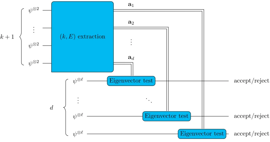
test whether |ψi is an eigenvector of Wai for every i = 0, . . . , k−1 (by performing Weyl measurement twice on two independent copies of |ψi), and accept iff all tests accept. we will give a family of natural protocols that has three parameters:

• the number of times Bell sampling is performed,

k+ 1

ψ⊗2

ψ⊗2

ψ⊗2

Bell Sampling .. . Bell Sampling Bell Sampling

xk

x1

x0

E⊆ {0,1, . . . , k}2

ad

.. .

a3

a2

a1

d

Figure 5.1: A Bell difference extraction parameterized byk∈NandE⊆[k]2, with|E|=d.

• the number of Weyl measurements performed for each WeylWx+y test.

We will define this family of stabilizer testing protocols more formally in Section 5.1. In Section 5.2, we will prove a lemma that helps us analyzing the protocols of the form (k, `, E). This lemma is a generalization of Lemma3.16that we used in Chapter 3 to prove an alternative analysis of the 6-copy algorithm. In Section 5.3, we analyze some interesting stabilizer testing protocols. We prove an upper bound of the error probability for each protocol which depends on the parameters of the protocol. In Section 5.4, we will use the bound that we have obtained to see how each parameter affects the bound to understand the performance of this family of stabilizer testing protocols and answer the Question (∗).

5.1

A natural stabilizer testing protocol

For every positive integer k, let [k] = {0,1, . . . , k}. We define a generalization of Bell difference sampling [GNW17] as follows.

Definition 5.1(Bell difference extraction). Letk∈_N. SupposeE⊆[k]2 _{is non-empty and}