Applying model parameters as a driving force to a
deterministic nonlinear system to detect land cover
change
B.P. Salmon, D.S. Holloway, W. Kleynhans, J.C. Olivier and K.J. Wessels
Abstract—In this paper we propose a new method for extract-ing features from time series satellite data to detect land cover change. We propose to make use of the behavior of a determin-istic nonlinear system driven by a time dependent force. The driving force comprises a set of concatenated model parameters regressed from fitting a model to a MODerate-resolution Imaging Spectroradiometer time series. The goal is to create behavior in the nonlinear deterministic system which appears predictable for time series undergoing no change, while erratic for time series undergoing land cover change. The differential equation used for the deterministic nonlinear system is that of a large amplitude pendulum, where the displacement angle is observed over time. If there has been no change in land cover the mean driving force will approximate zero, hence the pendulum will behave as if in free motion under the influence of gravity only. If however there has been a change in land cover this will for a brief initial period introduce a non-zero mean driving force, which does work on the pendulum, changing its energy and future evolution which we demonstrate is observable. This we show is sufficient to introduce an observable change to the state of the pendulum, thus enabling change detection. We extend this method to a higher dimensional differential equation to improve the false alarm rate in our experiments. Numerical results show change detection accuracy of nearly 96% when detecting new human settlements, with a corresponding false alarm rate of 0.2% (omission error rate of 4%). This compares very favourably with other published methods, which achieved less than 90% detection but with false alarm rates all above 9% (omission error rate of 66%).
Index Terms—Nonlinear detection, Remote sensing, Time se-ries
I. INTRODUCTION
It is estimated that more than a third of the Earth’s land surface has been transformed by anthropogenic activities [1]. These changes affect the environment driven by socio-economical factors. These changes include deforestation, agri-cultural expansion and urbanization which have significant impact on hydrology, ecosystems and climate [2], [3]. The increase in human population is a major driver of settlement expansion, which applies further pressure on the remaining natural resources [4]. The growing human population makes the detection of newly formed human settlements the focus of this study.
B.P. Salmon, D.S. Holloway and J.C. Olivier are with the School of Engineering and ICT, University of Tasmania, Australia
Email: [email protected]. Tel: +61 3 6226 7665. Fax: +61 3 6226 7247
K. Kleynhans is with the Department of Electrical, Electronic and Computer Engineering, University of Pretoria and Remote Sensing Research Unit, Meraka Institute, CSIR, Pretoria, South Africa
[image:1.612.330.547.193.461.2]K.J. Wessels is with the Remote Sensing Research Unit, Meraka Institute, CSIR, Pretoria, South Africa
Figure 1. Land cover change detected in the town of Modimolle (24◦41008.4700S,28◦24045.7500E) located in the Limpopo province, South Africa. The Quickbird image at the top was taken on 24 April 2006 and the bottom on 3 November 2012 (Courtesy of GoogleTM Earth). A change in land cover type is shown in the pink box, while adjacent areas only undergo a seasonal change which is shown in the green box.
Historically, change detection relied largely on image inter-pretation by analysts. Owing to the vast amounts of satellite imagery that are available, machine learning methods are now widely regarded as the most viable option for classification and change detection [5], [6]. The use of machine learning methods enables change detection, which encompasses the quantifica-tion of temporal phenomena from multi-date imagery most commonly acquired by satellite-based multi-spectral sensors [7]. Detecting land cover change using machine learning methods can reduce human interaction and enable large data sets to be potentially processed in a fraction of the time.
images acquired at high temporal frequency should provide the ability to distinguish between change events and phenological cycles [9]. Capitalizing on the high temporal sampling rate which captures the dynamics of different land cover types provides information on the seasonal dynamics in the form of a time series [10]. Incorporating this temporal information into a change detection algorithm allows the method to distinguish between land cover conversion and natural seasonal variations. Over the last decade numerous time series change detection methods have been developed to operate on various satellite images. These methods are limited by the number of images available in the study area and the type of change investigated. Medium resolution satellite imagery is becoming more com-mon in time series analysis, such as the Landsat time series stack which consist of a single image every year [11]. The Vegetation Change Tracker (VCT) algorithm was applied to this stack to detect changes in forests for every year from 1984 untill 2006. This was adequate as undisturbed forests typically maintain stable spectral reflectances over many years, while non-forest land cover types have both seasonal and inter-annual variability [11]. Similarly a linear spectral mixture analysis was used on 8 Landsat images to improve the net loss in sub-Saharan African forests between 1995 and 2011 [12]. In recent work an iteratively re-weighted multivariate alteration detection (IRMAD) was used to detect land cover change in monthly composited Landsat images between 2008 and 2011 [13]. The areas identified as no-change was then supplied to a random forest classifier for classification.
If longer time series are required or larger study areas are surveyed then there is a need for high temporal and wide swath acquisitions of coarse resolution satellite imagery, such as MODerate-resolution Imaging Spectroradiometer (MODIS). An example of surveying a large study area was the inves-tigation of dimensionality reduction in multi-temporal remote sensing images using principal component analysis for land cover classification on MODIS for over 204 training sites [14]. This data set consist of 28 images with an expectation maximization algorithm used to compute missing data. In Bangladesh thousands of hectare of Aus rice was monitored using MODIS [15]. The high temporal revisit time of MODIS allowed temporal and spatial growth profiles for eight sites to be created between May and July 2010. In [16], the conversion of forest to grassland and cropland to grassland was investigated using MODTrendr. MODTrendr is a temporal segmentation algorithm which uses trajectory segmentation to determine change in slopes within time series.
The objective of our research is to detect new human settlements which are unplanned and unregulated, which are quite common in the developing world. This means we do not know where and when these settlements will be erected, so that use of high resolution imagery to detect change is computationally prohibitive and impractical. Thus the goal is to detect potential new human settlements using coarse resolution imagery at moderate computational cost, which will then allow us to task high resolution satellites for confirmation and detailed mapping of change events so detected. We need wide swath images to scan large areas for possible changes as well as high temporal revisit times as these settlements can
quickly be constructed, often in a matter of weeks.
New settlements were reliably detected in our study area using a neural network trained on short-term Fourier transform extracts [17]. This was shown to be a robust approach to extracting meaningful features which most temporal sliding window methods do not comply with [18]. A windowless approach using an extended Kalman filter to extract features from a time series was shown to produce similar results [19]. However all the methods operate on the basis of extracting descriptive features from a time series and present it to a machine learning method. A major challenge for most change detection algorithms is to attain high change detection accu-racy (true positives) while maintaining a low false alarm rate (false positives). This process usually entails the extraction of features which generally improves the ability to learn patterns associated with change.
These methods all rely on significant changes in the spectral reflectance over a short time interval which the machine learning method can identify. The construction time however of these new settlements can vary significantly, which reduces the detection accuracy. Lowering the thresholds to compensate for this reduction unfortunately increases the false alarm rate. In this paper we propose a new paradigm for detecting change, yet maintaining a low probability of false alarm. The proposed method creates new features by applying the extracted features (regressed model parameters) as a driving force to a deterministic nonlinear system. We will demonstrate that the output or state of the deterministic nonlinear system is predictable for geographical areas that are experiencing no land cover change, and unpredictable (erratic) when there is land cover change. Thus the observed state of the nonlinear system presents a straightforward method for change detection. This we will show is the case regardless of the rate of change [20] as a time series undergoing land cover change is time-dependent and has non-stationary properties [21].
The paper is organized as follows. Section II discusses the study area and data set. In section III we present the new proposed method, and in section IV our experimental results are presented. Section V presents the conclusions.
II. STUDY AREA AND LAND COVER DATA
The Limpopo province is located in the northern part of South Africa and is largely covered by natural vegetation that is used by the local population as grazing for cattle and wildlife. The development of settlements in the area is currently one of the most pervasive forms of land cover change and to a large extent informal and unplanned. Mean annual maximum temperature is 29◦C, mean annual minimum temperature is 15◦C and mean annual precipitation during the last 30 years is below 600 mm with 84% occurring between October and March. The province experienced a drought during 2002 [22].
regions was used as a control set to moderate between analysts. The analysts had assess to various high resolution satellite imagery for validation which is summarized as follows:
• SPOT2 imagery at 20 m spatial resolution for year 2000– 2001,
• SPOT5 imagery at 5 m spatial resolution for year 2006– 2008,
• Quickbird imagery (courtesy of GoogleTM Earth) at 0.65 m panchromatic, 2.62 m multi-spectral (at nadir) spatial resolution for the period 2001–2013.
Each analyst had to map out various polygons of change and no-change using all the imagery available. The number of images available varied significantly between geographical areas but there were always at least two images available; SPOT2 and SPOT5 images. Due to this variation, determining the exact date of change was impossible. Software was then used to determine the percentage overlap between mapped polygons and MODIS pixels. An investigation from past work concluded that methods proposed for change detection could detect change if more than 70% of MODIS pixels were changed, which we used as a benchmark to test our new proposed method [19]. The polygons varied significantly in size from single MODIS pixels to several dozens of pixels. In our analysis we applied cross validation to avoid common pitfalls in evaluating methods [23]. This allowed different polygons to be included in the validation phase of inspecting various methods. The study area, which was validated by visual inspection, had geographical areas experiencing no change of natural vegetation and human settlement covering an area of 558 km2(2232 MODIS pixels). The study area also contained geographical areas where land cover changed and this class covered 29.25 km2 (117 MODIS pixels).
The time series of the MODIS pixels identified in this work were extracted from the 500 m MCD43A4 land surface reflectance product. It was used because it offers nadir and bidirectional reflectance distribution function (BRDF) adjusted spectral reflectance bands [24]. For each pixel a time series was extracted from all seven spectral bands of the 8-day composite MODIS MCD43A4 data set (year 2000–2012). The quality flags in the MODIS data were used to identify cases where quality was low due to persistent cloud cover (or other atmospheric factors) over the 8 day period of data collection [24]; these samples were replaced by interpolating through temporal neighbors using a cubic spline.
III. PROPOSEDCHANGEDETECTIONMETHOD
A. Feature extraction
The ability to differentiate between seasonal variations and land cover change makes time series analysis very appealing [7]. We start our discussion with a traditional approach to detect land cover change in a time series. A N-sample time series of reflectance values for a given pixel is
~
xb={xn,b}nn==1N ={x1,bx2,b. . . xN,b}, (1)
where the time index is denoted by n ∈ [1, N] and the spectral band byb∈[1, . . . ,7]. Machine learning methods can detect change in a time series by considering either the entire
time series or a set of sub-sequences extracted with a sliding window [18]. The ability of the machine learning method to detect change is improved when more descriptive features are extracted.
A common feature extraction approach is to fit a parametric model to a time series with a suitable regression algorithm. The regressed model parameters are then used as input to the machine learning method. The model can be fitted on the extracted sub-sequences with either a least squares [25] or a Fourier transform [18]. A windowless approach is also possible based on an extended Kalman filter using internal co-variance matrices [19]. The extended Kalman filter described in [25] was used to fit a triply modulated cosine model [26]. There is no restriction on the model used, except that it should be appropriate for the study area and model parameters must be regressed with a suitable algorithm.
For our study area the triply modulated cosine model is used and is defined as
xn,b=µn,b+αn,bcos(ωn+φn,b) +vn,b. (2)
The variable xn,b denotes the n-th observed value of the b
-th spectral band’s time series. Additive noise is denoted by vn,b ∼ N(0, σb2). The angular frequencyω is assumed to be
the same over all seven spectral bands and is computed with ω = 2πf, where f is based on the annual vegetation growth cycle. Given the eight daily composite MCD43A4 MODIS product,f was calculated to be 3658 . The cosine function was separately fitted on each spectral band at each time index to compute the following set of model parameters: the non-zero mean µn,b, the amplitude αn,b and the phase φn,b. Previous
studies have found that the most relevant features for change detection in this study area are the non-zero mean µn,b and
amplitudeαn,b [19]. These derived model parameters form a
new pair of time series as
~
µb = {µn,b}nn==1N ={µ1,bµ2,b. . . µN,b}, (3) ~
αb = {αn,b}nn==1N ={α1,bα2,b. . . αN,b}. (4)
These time series are concatenated into matrices for multi-band analysis as
M ={~µb}bb=7=1=
µ1,1 µ2,1 . . . µN,1
µ1,2 µ2,2 . . . µN,2
..
. ... . .. ... µ1,7 µ2,7 . . . µN,7
, (5)
A={~αb}bb=7=1 =
α1,1 α2,1 . . . αN,1
α1,2 α2,2 . . . αN,2
..
. ... . .. ... α1,7 α2,7 . . . αN,7
. (6)
[17]
δc =
F(~µb) for mean parameter analysis F(~αb) for amplitude parameter analysis F(~µb, ~αb) for single band analysis
F(M,A) all spectral bands analysis
,
(7) whereδc denotes the change metric produced by the machine
learning function F. This metric is used to compute the true positive rate as P(c|δc, c) and false positive rate with P(c|δc, c). The variable c denotes change and c denotes no
change. This concludes the introduction to the conventional approach of detecting land cover change in a time series.
B. Using a nonlinear deterministic system to extract new features
In this section new input features are presented to be used by the machine learning functionF. These inputs are derived from the output state of a nonlinear system driven by a force P. Key requirements of this system are that it does not respond when there is no change in land cover, regardless of the values of~µb and~αb, but it will respond (ideally strongly) when there
is a change.
This first requirement is most simply achieved if we subtract the expected value, evaluated as a moving window average of recent past values, i.e. P = µn,b−E[µn,b] or P = αn,b−
E[αn,b], leaving essentially a stochastic process with a zero
mean when there is no change in land cover. This will be described more formally below. However if there is a change in land cover there will be a lag between µn,b and E[µn,b]
(or αn,b and E[αn,b]), so for a brief period there will be a
net action (or time integral) of the force acting on the system, producing a response which is readily detected (derivation in Appendix).
Regarding the second requirement, we propose a nonlinear system to provide improved detection compared with tradi-tional approaches. We propose a large amplitude pendulum as such a system, and will demonstrate that this provides higher true positive rates while significantly lowering the false positive rate. We propose to utilize the model parameters regressed from a time series and apply it as a driving forcePk
to a differential equation describing the pendulum as shown in Figure 2 at time index k. This driving force will move the pendulum’s bob away from its original periodic motion of swinging back and forth into a new state of oscillation.
A large amplitude pendulum is shown in Figure 2, which consists of a bob of massmsuspended from a massless rod of lengthLto a fixed frictionless pivot. The pendulum is released from an initial displacement angle θ0 and swing back and
forth with a periodic motion. The motion is dictated by all the tangential forces exerted on the bob which are the driving force and the tangential component of the gravitational force. By applying Newton’s second law for a rotational system, the motion of the pendulum in discrete closed-form is
∆2θ
k
∆k2 +C1sinθk =C2Pk, (8)
withC1= g∆t
2
L andC2 = −∆t2
[image:4.612.332.546.51.225.2]mL . The variableg denotes the
Figure 2. A large amplitude pendulum with no friction or air resistance.
gravitational acceleration. The variableθk denotes the angular
offset at time k relative to the static equilibrium position, i.e. relative to the bob hanging straight down, and ∆t is the time between successive samples (in this case 8 days). Counter-clockwise positions from the static equilibrium point are considered to have positive angles and clockwise positions with negative angles.
A small angle approximation of sinθk = θk is used to
compute the harmonic motion when the bob is released from a small initial displacement angle (|θ0|<30◦). This reduces
Equation (8) to a linear deterministic system. The period of a single swing depends only on the length of the rod and the strength of the gravitational field g. The initial displacement angle θ0 and the mass of the bob have no effect.
The small angle assumption however is not valid if the initial displacement angle θ0 is large (|θ0| ≥ 30◦), which
means the sinθk term remains in its nonlinear form shown
in Equation (8) and the motion should be tracked using a numerical method to approximate the solutions of the ordinary differential equation. The pendulum becomes “more” nonlin-ear for largerθ0. Although the pendulum motion is described
by a nonlinear response it is still completely predictable.
Let us formally define the driving force to illustrate the relation to the model parameters given in (3) and (4). The driving forceP~bµ for the time series~µb is
~
Pbµ={Pk,bµ }k=K k=1 ={P
µ
1,bP µ
2,b. . . P µ
K,b}, (9)
where in our experiments K N is arbitrarily large since the regressed model parameters are finite and the the motion of the pendulum can be observed as far into the future as is desired. Individual terms in the time series are
Pk,bµ =
µn,b−E[µn,b] for n=kandk≤N
0 otherwise . (10)
whereE[µn,b]is the expected value defined above. Similarly
the driving forceP~bα for the time series~αb is
~
Pbα={Pk,bα } k=K k=1 ={P
α
1,bP α
2,b. . . P α
with
Pk,bα =
αn,b−E[αn,b] for n=kandk≤N
0 otherwise . (12)
Without loss of generality all following discussion about the driving force P~b will hold for both P~
µ b andP~
α
b. The angular
offset θk is dependent on the applied driving force. A vector
containing the complete periodic motion of the pendulum for a particular driving force is
~
θb(P~b) = {θk,b({Pi,b}ii==1k)}
k=K k=1
= {θ1,b({Pi,b}ii=1=1). . . θK,b({Pi,b}ii==1K)}.(13)
Based on the conditional equations shown in Equations (10) and (12), there are two phases to the pendulum motion which will be presented in detail in this section.
Phase I (applied driving force), initiation of the pendulum over time periodk= [1,2, . . . , N], indicating that N samples from the time series are available. Over this period only minimal change in θ is desired, and is achieved by making the pendulum period greater thanN (controlled by adjusting the value ofC1). If there has been no change in land cover the
mean driving force will approximate zero, hence the pendulum will behave as if in free motion under the influence of gravity only. This is a state we are able to recognise as theno change
state as its known a priori.
On the other hand, if there has been a change in land cover this will for a brief period introduce a non-zero mean driving force, which does work on the pendulum, changing its energy and future evolution. This is sufficient to introduce a very apparent and observable change to the state of the pendulum at the end of Phase I, which, as demonstrated in the Appendix can significantly change its natural period of oscillation. The degree to which this occurs depends on the degree of non-linearity, which can be controlled by the initial conditions to Phase I. For example, at an amplitude ofθmax= 178◦a 0.01%
change in the pendulum’s energy produces approximately a 4% change in the pendulum’s period. This is in stark contrast to the well known fact cited above that for small to moderate amplitude (θmax≤30◦) the period is essentially independent
of amplitude. Thus the driving force magnitude (governed by C2) need only be small to produce the necessary change in
energy, in fact it needs to be small to ensure that the pendulum state does not change when there is no change in land cover. During Phase II (driving force removed), referred to as
separation of states, the pendulum is unforced and allowed to swing freely (Pk,bµ = 0for k > N), with initial conditions being the state of the pendulum at the end of Phase I. We have shown that for a highly nonlinear pendulum (an amplitude of motion θmax →π) if there has been a change in land cover
the change of state by the end of Phase I will significantly change the pendulum’s free oscillation period. Of course there is some separation in Phase I, but since this occurs over a finite and relatively small time this separation is not yet detectable at the start of Phase II. However over a small number of oscillations the states due to no-change or change will quickly separate, and the separation will be straightforward to observe, presenting us with a change detection strategy.
(a) Pendulum’s angle of displacement over time given driving forces derived from all the MODIS time series undergoing no land cover change.
[image:5.612.333.537.63.227.2](b) Pendulum’s angle of displacement over time given driving forces derived from all the MODIS time series undergoing land cover change.
Figure 3. The observed angle of displacement given the driving force of model parameter αk,2 on the pendulum. The extraction ofαk,2 from no
change MODIS time series shown in (a) and change MODIS time series in (b).
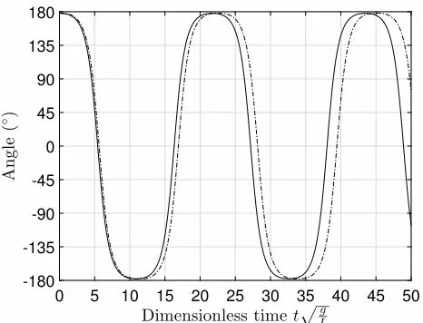
For example (see Figure 8), at an observation time of 2.25 periods the pendulum position will be0◦with no driving force. If the initial amplitude is set to θmax = 178◦ and a driving
force exists that is scaled to increase the system energy by only 0.01% then the new angular displacement at the same observation time will be 142◦. This is explained further in the Appendix and shown in Figure 8, and is because of the sensitivity of the period to the driving force and steepness of the θ versus time relationship around θ = 0. It also has the desirable feature of being relatively insensitive to larger changes in the driving force since above150◦the motion curve is quite flat and can tolerate significant phase shifts before returning below this value (e.g. dimensionless times in the range 40–47 in Figure 8 — thus it matters that change has occurred, but not by how much).
land cover change when present. Equation (7) shows how a machine learning method is used to detect change using model parameters. We change the input features to the periodic motion path as
δc(P) =
F(~θb(P~b)) for single parameter analysis F(~θbµ(P~b), ~θbα(P~b)) for single band analysis F(Θµ,Θα) all spectral bands analysis
,
(14) where δc(P) denote the change metric produced by the
machine learning function F. The spectral bands are paired for multi-band analysis as Θµ = {~θµ
b(P~b)}bb=7=1 and Θ
α =
{~θα
b(P~b)}bb=7=1. The conjecture is a disturbance to the periodic
motion of the pendulum would be a more descriptive feature to the machine learning method than the original regressed model parameters.
Lemma 1. The characteristics of a differential equation can be investigated with the aid of a phase plane plot, which illustrates the limit cycles of the solutions. A three-dimensional phase plane representation that is autonomous can be de-rived for Equation (8) as shown in [27]. The Poincar´e-Bendixson theorem states that a differential equation with a three-dimensional phase plane can be chaotic [28]. Hence Equation (8) is a nonlinear deterministic system that can exert an erratic response.
According to Lemma 1, an erratic response is possible given a suitable time dependent driving force. However given the 8-day acquisition rate of MODIS the change in the time series might only be observed for a few time samples. Here observing the pendulum over infinite time (KN) is highly advantageous as the pendulum is sensitive to changes in the initial conditions, where a small change in Phase I can result in large differences in Phase II. This means the differences in the solutions for change and no change time series should become more clear ask→ ∞. This effect can be even further enhanced by increasing the non-linearity with θ0→180◦ (θ0→π).
Thus the problem of detecting change in the pendulum’s motion path can be formulated as a binary hypothesis test for kN as:
H0:~θb(P~b)|~xb(c) no change in time series~xb
H1:~θb(P~b)|~xb(c) change in time series~xb (15)
Testing hypothesisH1is problematic as~θb(P~b)|~xb(c)could be
unpredictable in practice. Hence only hypothesisH0is deemed
testable as it is predictable and if rejected then we can assume H1. Thus hypothesisH0is formulated as
p~θb(P~b);H0
=
~
θb(~Pb)−~θb(~0)
=
~
θb(P~b)−~θb∗
< γ,
(16) where~θb∗denotes the expected motion path of the pendulum if the initial angleθ0and initial angular velocity
dθ(0)
dt is known
and no driving force is exerted (Pk,b= 0,∀k). The variableγ
is used to set the true positives and false positive rates. This binary hypothesis test suggest that a single parameter — given a single pendulum’s motion path — can be solved
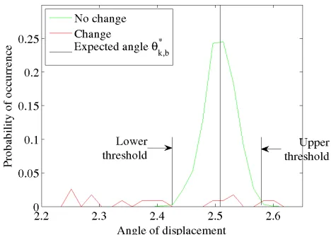
(a) Distribution of displacement angles at the point of index shown in Figure 3.
[image:6.612.320.554.274.440.2](b) An enlarged view of the distribution with the lower and upper threshold inserted.
Figure 4. An illustration of the displacement angle given the exertion of amplitude model parameter of the second spectral band on the pendulum at time index 5670 (point of interest in Figure 3). The expected displacement angle at this time index is 2.507 radians and is denoted with a black dirac delta function. The distribution of the no change MODIS time series is shown in green around the expected displacement angle and change MODIS time series in red. The naive Bayes threshold for the lower threshold is computed as 2.42 radians and upper threshold as 2.58 radians. The threshold produce a change detection accuracy of 95.6% with corresponding false alarm rate of 0.9%.
optimally with a naive Bayes classifier as a change detection algorithm. A single band analysis (mean and amplitude pa-rameter combined) in Equation (14) using both the mean and amplitude model parameters can be viewed as a 3-dimensional space with 2 degrees of freedom which we solved using a Support Vector Machine (SVM). The same holds for the all seven spectral band analysis using both parameters which is 15-dimensional with 14 degrees of freedom for parameter sets {Θµ,Θα}.
Figure 5. Land cover change detected in the town of Dairing (23◦49022.7300S,29◦21027.5500E) located in the Limpopo province, South Africa. The Quickbird image on the left was taken on 23 April 2001 and on the right on 14 April 2013 (Courtesy of GoogleTMEarth). This detection was made on a
small existing settlement growing borders and internal increase in dwellings. All these pixels were successfully detected by our method.
differential equation toM pendulums swinging independently. An advantage of using the independence property is that each pendulum is independent in time to each other. This allows us to investigate each pendulum’s displacement angle at different time indices. This is a powerful property but for the sake of simplicity will not be explored in our analysis as we will restrict ourselves to a single time index for all our experiments.
IV. EXPERIMENTAL SETUP AND RESULTS
A. Setting of parameters and illustrative example
We will start this section by first discussing how to set up the pendulum, followed by a illustrative example and conclude with experimental results.
A requirement was to make the pendulum appear pre-dictable, which implies fixed initial conditions. The pendulum was set with the following conditions: (1) an initial displace-ment ofθ0= 178◦(3.10 radians), (2) initial angular velocity of
∆θ0
∆k = 0, (3)C1= 3.42×10 −6(C
1= g∆t
2π
180◦L, using description in Appendix, we arbitrarily set g = 9.8 m/s2, ∆t = 1
50,
L= 20andm= 1) and (4)C2= 3.49×10⁻⁷ (C2=−∆t
2
mL,
for more description on how to set these parameters please refer to the following paragraphs and the Appendix). The length of the driving force was set to N = 550 as we had 12 years of MODIS data available in our experiments and the number of observations of the pendulum was arbitrarily set high to K= 20000.
C1determines the linear (or minimum) period of oscillation
of the pendulum (Tmin= 2π/
√
C1), which we suggest should
be large compared with the duration of Phase I. This is so that work done by the driving force is either only positive or only negative. When a land use change occurs the expected value of the driving variable will lag the changing actual value, so the driving force will have a constant sign. Work done on the pendulum is the product of this with displacement, so if Tmin
is too short and the pendulum begins to return during Phase I (as would be the case if C1 is too large) there will be both
positive and negative work done on the pendulum, producing cancellation of energy input, hence its change in energy would not be as great as it could be, and could even at times be nearly
zero. This would compromise the nonlinear system’s ability to detect the change.
SettingC2does also change the behavior quite significantly
as it can either amplify or negate the effects of the driving force. A pendulum can complete multiple 360◦ cycles if too much driving force is applied (largeC2). This is undesirable
as the number of completed cycles must be recorded for each individual driving force in the analysis and the properties of the differential equation are negated. The effect of the driving force could also be severely attenuated ifC2 is small, which
will hinder the possibility of measuring any characteristics of the driving force and make Equation (8) appear more linear deterministic. C2 should be selected to ensure a constrained
motion in the pendulum such that θk ∈(−π, π),∀k and that
a desirable response can be observed.
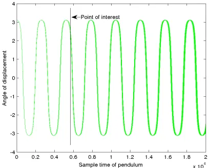
For an illustrative example, shown in Figure 3, let us use the regressed amplitude parameter of the second spectral band to drive a pendulum which is
~
α2={α1,2 α2,2. . . α550,2}, (17)
with corresponding driving force
~
P2α=n{αk,2−E [αk,2]}kk=550=1 {0}
k=20000
k=(551)
o
. (18)
Using this driving force we can approximate the solution of Equation (8) using a fourth-order Runge-Kutta method to derive a time series of displacement angles as
~
θ2(P~2α) ={θk,2({Pi,α2}ii==1k)}kk=20000=1 . (19)
The conjecture was that the displacement angle ~θ2(P~2α)
Figure 6. Land cover change detected in the suburb of Polokwane Extension 28 (23◦54031.4100S,29◦30024.8000E) located in the Limpopo province, South Africa. The Quickbird image on the left was taken on 3 June 2001 and on the right on 25 September 2011 (Courtesy of GoogleTMEarth). Only the top right
MODIS pixel was flagged as changed. The three remaining pixels had to little change in the geographic footprint to be detected.
samples undergoing non-stationary change has a notable net force exertion on the pendulum.
An arbitrary point of k = 5670 was selected as an illus-trative example—denoted as ‘point of interest’ in Figure 3. At this selected point the expected angle θ∗k,b is denoted with a black Dirac delta function in Figure 4. A distribution for time series undergoing no land cover change is shown in green. It is clear that this distribution is located in close proximity to the expected angle. Similarly a distribution for time series undergoing land cover change is shown in red. This distribution however is scattered and can easily be detected by placing an upper and lower threshold around the no change distribution. A Bayesian approach was used to set the two thresholds given a fixed permitted number of false positives. Estimating the thresholds can be done with any machine learning method and is denoted as
δc(P~2) =F
~ θ2(P~2α)
. (20)
In this example a true positive rate of 95.6% was found with corresponding false positive rate of 0.98%.
Investigating M-pendulum simultaneously will require the aid of a support vector machine. Producing meaningful results will require proper presentation of the displacement angles to the SVM [18]. As land cover change is assumed to appear erratic, it would be infeasible to train a classifier to classify this behavior. Instead the support vector machine was used to determine the threshold plane for the responses generated by no land cover change time series and treated the land cover change responses as anomalies. In our work we set up a SVM with a Gaussian radial basis function kernel and used tenfold cross validation to set the influence of the support vectors used and penalty term to trade off the incorrect classifications when deriving the decision surface.
B. Experimental results
The mean and amplitude parameter of all the seven spectral bands were used in separate experiments as driving force. The difference in pendulum oscillation stabilized as k → K and
kN, which means the separation of states in Phase II has taken full effect and no more difference could be found. True positive rates (change detection accuracy) and false positive rates (false alarms) at this point are reported in Table I.
Spectral bands 2, 5, 6 and 7 offered the most promising results on our labeled data set. The amplitude parameter of the second spectral band had the highest detection accuracy at a fixed false positive rate. The mean parameterµk,1 of spectral
band 1 barely offered true positive rates above 70% with a corresponding false positive rate of 10%. Spectral bands 3 and 4 offered unacceptable low true positive rates. The commission and omission error rate on these four spectral bands support this claim.
However, even though the other spectral bands offer poor performance they can still offer valuable information when a supervised classifier like a SVM classifies in a multi-dimensional space. It either has the ability to assist in improv-ing the true positive rate [17] or it can lower the false positive rate [25]. Our experiments found that the false positive rate was further reduced as shown in Table II when a SVM was used on the 14-dimensional pendulum.
An overall true positive rate of 96% was observed with a ten-fold cross validation and a corresponding false positive rate of less than 0.2% for the 14-dimensional pendulum. This was a significant improvement when compared to previous work done on this study area (Table II).
Table I
THE AVERAGE CHANGE DETECTION ACCURACY(TRUE POSITIVES RATES)ALONG WITH THEIR CORRESPONDING FALSE POSITIVES RATES MEASURED ON THE LABELED DATA SET FOR ALL SEVEN SPECTRAL BANDS IS GIVEN ON THE TWO MODEL PARAMETERS. THE OVERALL ACCURACY,COMMISSION
ERROR AND OMISSION ERROR RATE IS ALSO PROVIDED.
Spectral Parameter True positives False positives Overall Accuracy Commission error Omission error
band (%) (%) (%) (%) (%)
Band 1 µk,1 56.9 0.98 96.9 43.1 24.7
αk,1 25.9 0.98 95.4 74.1 41.9
Band 2 µk,2 92.2 0.98 98.6 7.8 16.8
αk,2 95.6 0.98 98.8 4.4 16.3
Band 3 µk,3 0.8 0.98 94.1 99.2 95.9
αk,3 0.0 0.98 94.0 100.0 100.0
Band 4 µk,4 14.6 0.98 94.8 85.4 56.2
αk,4 2.6 0.98 94.2 97.4 87.8
Band 5 µk,5 81.0 0.98 98.1 19.0 18.75
αk,5 76.7 0.98 97.9 23.3 19.6
Band 6 µk,6 87.1 0.98 98.4 12.9 17.6
αk,6 78.4 0.98 97.9 21.6 19.2
Band 7 µk,7 88.7 0.98 98.5 11.3 17.4
αk,7 93.9 0.98 98.7 6.1 16.6
Table II
ACOMPARISON BETWEEN DIFFERENT CHANGE DETECTION ALGORITHMS ON THE LABELED DATA SET.
Algorithm True positives False positives Overall Commission Omission
(%) (%) Accuracy (%) error (%) error (%)
Annual NDVI differencing method [7] 69 13 86 31 78
Multilayer perceptron 2-bands method [17] 79 17 83 21 80
Multilayer perceptron 7-bands method [17] 87 9 91 13 66
EKF spatial window method [19] 89 13 87 11 74
Best 1-dimensional pendulum 96 1 99 4 16
14-dimensional pendulum 96 0.2 99 4 4
of the methods were hindered as the spectral differences were small in the bands undergoing land cover change. A spatial approach yielded higher change detection accuracy in the study area, such as the EKF spatial window method [19]. This method computed the differences between neighboring pixels to detect change. This improved the change detection accuracy to 89% with false alarm rate of 13%. However, none of these methods could compete with a single pendulum let alone a 14-dimensional pendulum. The best performing pendulum used the amplitude parameter of the second spectral band as driving force which obtained a true positive rate of 96% with a false positive rate of 1%.
The increase in change detection accuracy compared to other methods was investigated. One of the improvements that was found is shown in figure 5. In the town of Dairing there was a growth in the borders as is seen in the illustration, but also a growth in the internal number of dwellings. All nine pixels in this illustration was detected with the proposed approach which we defined as success. We also investigated other areas which we knew had small changes compared to a relative size of a MODIS pixel as shown in figure 6. These high resolution imagery show significant change in the upper right MODIS pixel and several minor changes in the remaining three pixels. Only the upper right pixel was declared as changed by our method, which made us aware of the remaining three pixels upon inspection of the high resolution image. This showcases how coarse resolution satellite imagery can be used to task high resolution satellites to find new
settlement expansions.
V. CONCLUSIONS
In this paper we present a new descriptive feature to assist machine learning method to detect change in a time series. The descriptive feature is derived by exerting a regressed model parameter as a driving force to a deterministic nonlinear system. The large amplitude pendulum was biased to exhibit a nonlinear deterministic response for time series undergoing no land cover change and appeared erratic for time series undergoing change.
It was shown that a land cover change prediction signifi-cantly improved with reported change detection accuracy of 96% when using all seven spectral bands of MODIS with false alarms as low as 0.2% and omission error of 4%. This compares with a result of less than 90% detection but with false alarm rates all above 9% and omission errors above 66% for other published methods.
Normalised energy E mgL
0 0.2 0.4 0.6 0.8 1 1.2 1.4 1.6 1.8 2
A m p li tu d e ( ◦) 0 30 60 90 120 150 180
(a) Effect of energy on amplitude.
Amplitude (◦)
0 30 60 90 120 150 180
N o rm a li se d p er io d
T 2π
p g L 0 0.5 1 1.5 2 2.5 3 3.5 4
[image:10.612.60.293.49.445.2](b) Effect of amplitude on period.
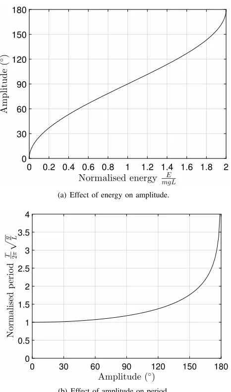
Figure 7. Showing how the pendulum’s energy affects its period by increasing its amplitude.
We postulate various different Earth observed processes and changes may be better expressed or viewed by modulating the correct differential equation.
APPENDIX
The governing equation in continuous time for the motion of the large amplitude pendulum of Figure 2 is
d2θ
dt2 +C1sinθ=C2P(t) (21)
with C1 = Lg and C2 = mL−1. For an unforced motion P(t) = 0 ∀t starting from rest dθ0
dt = 0
with initial angular displacement θ0, the problem reduces to solving
C3
d2θ
dt2 + sinθ= 0 (22)
with C3 = Lg. To analytically derive the unforced natural
period of the large amplitude pendulum we reduce (22) to a first order equation by multiplying it with dθdt
C3
d2θ
dt2 dθ dt =− dθ dt
sinθ. (23)
Then integrate (23) with respect to time with initials conditions of (22) to yield
C3 2 dθ dt 2
= cosθ−cosθ0, (24)
hence
dθ dt =−
r 2
C3
(cosθ−cosθ0). (25)
where the negative square root must be taken over the first half period to satisfy the initial conditions. The period of oscillation T is computed if Equation (25) is solved by separation of variables and integrating over a quarter of the period, which brings the pendulum to the vertical position at whichθ= 0, thus
− r C3 2 Z 0 θ0 dθ √
cosθ−cosθ0
= T
4 . (26)
Ifsinθ2 = sinθ0
2 sinφ, then a change of variable will replace
the integration limitsθ= 0andθ0withφ= 0andarcsin 1 =
π
2 respectively, which gives
1 2
r
1−sin2θ0 2 sin
2φ dθ = sinθ0
2 cosφ dφ (27)
cosθ−cosθ0 =
1−2 sin2θ0 2 sin
2φ
−
1−2 sin2θ0 2
= 2 sin2θ0 2 cos
2φ .
(28)
which simplifies after some reduction to
T = 4pC3
Z π2
0
dφ
q
1−sin2θ0
2 sin 2φ = 4 s L gK sin2θ0
2
,
(29) whereKis the complete elliptic integral of the first kind [29]. Note that K(0) = π2 and K0(0) = 0, hence we recover the classic small amplitude pendulum period solutionT = 2πqLg independent of amplitude.
As confirmed by (25), the total energy of the pendulum system in the absence of a driving force is constant and equal to the potential energy at the maximum amplitude, namely E =mgL(1−cosθ) if the potential energy is referenced to the static equilibrium positionθ= 0. As shown in Figure 7(a), if the pendulum’s amplitude is close to 180◦then a small input of additional energy may change the amplitude significantly. Figure 7(b) shows that at these angles the period is also very sensitive to the amplitude, so this input of energy will in turn significantly change the pendulum’s period.
If we now change the one initial condition of dθ0
dt(0) = −ω0, how will it alter the pendulum angle θ(t) at arbitrary
time? We assumeω0 is positive, so the pendulum has already
[image:10.612.313.569.347.520.2]Dimensionless time tpLg
0 5 10 15 20 25 30 35 40 45 50
[image:11.612.59.292.52.230.2]A n g le ( ◦) -180 -135 -90 -45 0 45 90 135 180
Figure 8. Showing the effect of a 0.01% increase in energy from an initial displacement of 178.0000◦(solid line) to 178.3608◦(broken line). Time is normalised such that the linear (small amplitude) period is2π. At an amplitude of 178◦the actual period is 3.460 times the linear period (t
q
g
L= 21.74).
energy is less than2mgL, hence based on energy conservation we can define an amplitude θmax satisfying
cosθmax= cosθ0−
1 2C3ω
2
0. (30)
We note therefore that the period is now
T = 4 s
L gK
sin2θmax 2
. (31)
Lettrefdenote the reference time which is the last time before
t= 0 at whichθ=θmax. In order to retain the negative sign
on the right of (25) we define a reduced timeτ as the shortest time aftertref at whichθ(τ) =θ(t). Given that the pendulum
motion is periodic, this is
τ =
mod(t−tref, T) mod(t−tref, T)< T2
T−mod(t−tref, T) otherwise
,
(32) which is always in the range 0 ≤τ < T
2. In the manner of
deriving Equation (26) we integrate (25) with modified limits and divide the integral into two parts to obtain
τ = −
r C3 2 Z 0 θmax dθ √
cosθ−cosθmax
+ Z θ(t)
0
dθ √
cosθ−cosθmax
, (33)
−tref = −
r C3 2 Z 0 θmax dθ √
cosθ−cosθmax
+ Z θ0
0
dθ √
cosθ−cosθmax
. (34)
The appropriate change of variable is now
sinθ 2 = sin
θmax
2 sinφ , (35)
and the first integral is just T4, so following the same approach
as above,
τ = T
4 − p
C3
Z ϕτ
0
dφ
q
1−sin2θmax
2 sin 2φ = T 4 − s L gF
ϕτ\ θmax
2
(36)
where sinϕτ =
sin(θ/2)
sin(θmax/2) and F(ϕ\α) = F(ϕ|m) is the (incomplete) elliptic integral of the first kind, defined by Abramowitz and Stegun [29, S17.2] with m = sin2α. Note that K(m) =F(π
2|m) =F(
π
2\α). Similarly
tref=
s
L gF
ϕtref\ θmax
2
−T
4 (37)
whereϕtref =
sin(θ0/2)
sin(θmax/2).
In principle therefore, we can evaluate the angle at any given time by solving (36) givenτ from (32), (37) and (30).
For example, in the case of ‘no change’, after 214 periods τ= 0.250T exactly andθ= 0, but, as illustrated in Figure 8 (mentioned also above) where we started at an angle of 178◦ and increased the energy by 0.01%, the amplitude is increased to 178.3608◦, the period is increased by approximately 3.66% from 21.7396 to 22.5349 (the dashed line in the Figure 8), so we will haveτ= ( 2.25
1.0366−2)T = 0.1706Tandθ= 142
◦. This
is a dramatic change fromθ= 0for only a 0.01% increase in energy.
REFERENCES
[1] P. Vitousek, H. Mooney, J. Lubchenco, and J. Melillo, “Human domina-tion of earth’s ecosystems,”Science, vol. 277, pp. 494–499, July 1997. [2] R. DeFries, L. Bounoua, and G. Collatz, “Human modification of the landscape and surface climate in the next fifty years,”Global Change Biology, vol. 8, no. 5, pp. 438–458, 2002.
[3] J. Foleyet al., “Global consequences of land use,”Science, vol. 309, no. 5734, pp. 570–574, 2005.
[4] G. Daily and P. Ehrlich, “Population, sustainability, and Earth’s carrying capacity,”Bioscience, vol. 42, no. 10, pp. 761–771, November 1992. [5] D. Lu and Q. Weng, “A survey of image classification methods and
tech-niques for improving classification performance,”International Journal of Remote Sensing, vol. 28, no. 5, pp. 823–870, 2007.
[6] R. DeFries and J. Chan, “Multiple criteria for evaluating machine learning algorithms for land cover classification from satellite data,”
Remote Sensing of Environment, vol. 74, no. 3, pp. 503–515, 2000. [7] R. Lunettaet al., “Land-cover change detection using multi-temporal
MODIS NDVI data,”Remote Sensing of Environment, vol. 105, no. 2, pp. 142–154, November 2006.
[8] P. Coppin, I. Jonckheere, K. Nackaerts, B. Muys, and E. Lambin, “Digital change detection methods in ecosystem monitoring: a review,”
International Journal of Remote Sensing, vol. 25, no. 9, pp. 1565–1596, 2004.
[9] T. Grobleret al., “Using Page’s cumulative sum test on MODIS time series to detect land-cover changes,” IEEE Geoscience and remote sensing letters, vol. 10, no. 2, pp. 332–336, 2013.
[10] R. Lunetta, D. Johnson, J. Lyon, and J. Crotwell, “Impacts of imagery temporal frequency on land-cover change detection monitoring,”Remote Sensing of Environment, vol. 89, no. 4, pp. 444–454, 2004.
[11] C. Huang, S. Goward, J. Masek, N. Thomas, Z. Zhu, and J. Vogelmann, “An automated approach for reconstructing recent forest disturbance history using dense Landsat time series stacks,” Remote Sensing of Environment, vol. 114, pp. 183–198, 2010.
[13] K. Wesselset al., “Rapid land cover map updates using change detection and robust random forest classifiers,”Remote sensing, vol. 8, pp. 1–24, 2016.
[14] H. Glanz, L. Carvalho, D. Sulla-Menashe, and M. Friedl, “A parametric model for classifying land cover and evaluating training data based on multi-temporal remote sensing data,”ISPRS Journal of Photogrammetry and Remote Sensing, vol. 97, pp. 219–228, 2014.
[15] M. Sarker, M. Uddin, M. Ali, M. Akhand, and S. Rhaman, “Temporal monitoring of Monsoon crop using MODIS 16 day composite NDVI data for food security,”Journal of environmental sciences and natural resources, vol. 8, pp. 147–152, 2015.
[16] H. Yin, D. Pflugmacher, R. Kennedy, D. Sulla-Menashe, and P. Hostert, “Mapping annual land use and land cover changes using MODIS time series,”IEEE Journal of selected topics in applied earth observations and remote sensing, vol. 8, pp. 3421–3427, 2014.
[17] B. Salmonet al., “The use of a multilayer perceptron for detecting new human settlements from a time series of MODIS images,”International Journal of Applied Earth Observation and Geoinformation, vol. 13, pp. 873–883, 2011.
[18] B. Salmon, J. Olivier, K. Wessels, W. Kleynhans, F. van den Bergh, and K. Steenkamp, “Unsupervised land cover change detection: Meaningful sequential time series analysis,” IEEE Journal of selected topics in applied earth observations and remote sensing, vol. 4, no. 2, pp. 327– 335, 2011.
[19] W. Kleynhans et al., “Detecting land cover change using an extended kalman filter on MODIS NDVI time-series data,”IEEE Geoscience and Remote Sensing Letters, vol. 8, no. 3, pp. 507–511, May 2011. [20] C. Werndl, “What are the new implications of chaos for
unpredictabil-ity?”Br J Philos Sci, vol. 60, no. 1, pp. 195–220, January 2009. [21] W. Kleynhans et al., “Land cover change detection using
autocorre-lation analysis on MODIS time-series data: Detection of new human settlements in the Gauteng province of South Africa,”IEEE Journal of selected topics in applied earth observations and remote sensing, vol. 5, no. 3, pp. 777–783, June 2012.
[22] S. Mpandeli, E. Nesamvuni, and P. Maponya, “Adapting to the impacts of drought by smallholder farmers in Sekhukhune district in Limpopo province, South Africa,” Journal of Agricultural Science, vol. 7, pp. 115–124, 2015.
[23] S. Salzberg, “On comparing classifiers: Pitfalls to avoid and a recom-mended approach,”Data mining and knowledge discovery, vol. 1, no. 3, pp. 317–328, 1997.
[24] C. Schaaf et al., “First operational BRDF, albedo nadir reflectance product from MODIS,”Remote Sensing of Environment, vol. 83, no. 1/2, pp. 135–148, November 2002.
[25] B. Salmonet al., “Meta-optimization of the Extended Kalman Filter’s Parameters through the use of the Bias Variance Equilibrium Point Criterion,” IEEE Transactions on Geoscience and Remote Sensing, vol. PP, no. 99, pp. 1–16, November 2013.
[26] W. Kleynhans et al., “Improving land cover class separation using an Extended Kalman Filter on MODIS NDVI Time-Series Data,”IEEE Geoscience and Remote Sensing Letters, vol. 7, no. 2, pp. 381–385, April 2010.
[27] S. Strogatz, Nonlinear Dynamics and Chaos; with applications to physics, biology, chemistry and engineering, 1st ed. Cambridge, MA, USA: Westview Press, 2001.
[28] I. Bendixson, “Sur les courbes d´efinies par des ´equations diff´erentielles,”
Acta Mathematica, vol. 24, no. 1, pp. 1–88, 1901.
[29] M. Abramowitz and I. Stegun, Handbook of Mathematical Functions with Formulas, Graphs and Mathematical Tables, ser. Applied Mathe-matics. National Bureau of Standards, 1964, vol. 55.
B.P. Salmonreceived a M.Eng degree in electronic
engineering and a Ph.D. degree in electronic engi-neering from the University of Pretoria, South Africa in 2008 and 2012 respectively. He is presently a postdoctoral research fellow in the School of Engi-neering at the University of Tasmania. His research interests are information theory, coding theory, ma-chine learning and graph theory. He served as a guest editor for the IEEE Journal of Selected topic in applied earth observations and remote sensing.
D.S. Holloway has undergraduate degrees in both
music and civil engineering, with a University Medal in the latter. He received his Ph.D. in 1999 from the University of Tasmania, Australia, where he is now senior lecturer in structural engineering. He has held postdoctoral positions in applied mathematics and mechanical engineering. His current research interests span architectural acoustics, vibration and waves, fluid-structure interactions, ship hydrody-namics, thin shell buckling, and the boundary ele-ment method.
W. Kleynhansreceived a B.Eng., M.Eng. and Ph.D.
(Electronic Engineering) from the University of Pre-toria, South Africa as well as an MBA from Heriot-Watt University, Scotland. He is currently a principal researcher with the Remote Sensing Research Unit at the Council for Scientific and Industrial Research in Pretoria, South Africa and is also affiliated with the University of Pretoria. His research interests in-clude remote sensing, time-series analysis, wireless communications, statistical detection and estimation theory as well as machine learning.
J.C. Olivierreceived the Ph.D. degree in 1990 from
the University of Pretoria in Electrical Engineering. He is currently a Professor with the School of Engi-neering at the University of Tasmania, Australia. He was with Bell Northern Research (BNR) in Canada, and with Nokia Research Center in the United States. His research interests are in Estimation and Detection theory, as well as applications of Machine Learning. He serves as an Editor for the IEEE Trans. on Wireless Communications.
K.J. Wesselsreceived an M.Sc. in Landscape