The Influence of the Spatial Distribution of 2D
Features on Pose Estimation for a Visual Pipe
Mapping Sensor
Rahul Summan, Gordon Dobie, Graeme West, Stephen Marshall, Charles Macleod, Gareth Pierce
Abstract—This paper considers factors which influence the visual motion estimation of a sensor system designed for visually mapping the internal surface of pipework using omnidirectional lenses. In particular, a systematic investigation of the error caused by a non-uniform 2D spatial distribution of features on the resultant estimate of camera pose is presented. The effect of non-uniformity is known to cause issue and is commonly mitigated using techniques such as bucketing, however, a rigorous analysis of this problem has not been carried out in the literature. The pipe’s inner surface tend to be uniform and texture poor driving the need to understand and quantify the feature matching process. A simulation environment is described in which the investigation was conducted in a controlled manner. Pose error and uncertainty is considered as a function of the number of correspondences and feature coverage pattern in the form of contiguous and equiangular coverage around a circular image acquired by a fisheye lens. It is established that beyond 16 feature matches between the images, that coverage is the most influential variable, with the equiangular coverage pattern leading to a greater rate of reduction in pose error with increasing coverage. The application of the results of the simulation to a real world dataset are also provided.
Index Terms—Structure from Motion, Pipe Scanning, Bucket-ing.
I. INTRODUCTION
I
N sensors systems which employ cameras for motion estimation, it is commonly understood that uniform sam-pling of feature correspondences across an image yields more accurate estimates of relative motion in comparison to a biased distribution of points [1]. However, in scenes which contain highly variable textures in which feature points may be clustered together, uniform sampling may not be possible. This is of particular interest in the authors’ application area in which a sensor with a spherical field of view camera is used to perform Structure from Motion (SFM) within industrial pipelines. In such a setting, non-homogeneously distributed texture on the interior surface of the pipework can result in the majority of feature points being concentrated in one area of the image, see Figure 1. This shows a fisheye view down a pipe with the features correspondences highlighted by the line segments, the concentration of these features can clearly be seen. Such non-uniform texture can be caused by the surface finish of the material and or production method as well as defects including cracks and corrosion. The novel contribution of this paper is to provide a rigorous analysis, by way of simulation, of the relationship between the spatial distribution and number of features in the image and the accuracy of the resultant estimate of camera pose. In addition to this, thisresearch provides a design tool for implementers within this application area to assess the accuracy of their camera based sensor systems.
Monitoring the condition of structural assets through peri-odic inspection is of critical importance across many industries [2], [3]. Visual inspection of the interior surface of pipework in the nuclear and oil & gas industries is a priority inspection area in terms of safety and maintaining process flow by avoiding forced outages. Internal visual inspection is often used as a first pass inspection to identify areas of concern while volumetric imaging techniques such as ultrasound may be used to obtain dimensional data from the external surface of the pipe. However, due to access restrictions and potentially hazardous environmental conditions, it is desirable to use the visual data to also size defects. Such inspections are generally carried out by mounting a camera with associated illumination onto a push rod which is manually deployed into the pipework. Alternatively the camera may be driven through the pipe with a teleoperated tractor. In both cases, the inspection is a time consuming activity which is error prone especially in the manual deployment case due to probe orientation changes. Furthermore, by investigating a large structure using a camera with a relatively small field of view, it is very difficult to appreciate the nature and extent of surface defects.
The research presented herein is of interest for a particular engineering application concerned with visually mapping the internal geometry of pipework in the nuclear industry. In this application, a bespoke sensor system will be deployed into the pipeline and capture synchronised data from an on-board omnidirectional camera, laser line projector and inertial measurement unit (IMU). The objective is to then convert the resultant data into a 3D textured model of the surface of the pipe using SFM [4] assisted by orientation measurements from the IMU. Such a model will then be used to identify defects such as cracks, pits and loss of wall thickness that will inform a decision making process about the structural health of the pipe.
II. 3D MODELGENERATIONAPPLICATIONS INPIPE
INSPECTION
pipes using video captured through a fisheye lens deployed on a remotely operated tractor. Harris features are used in an structure from motion algorithm implementing bundle adjustment to estimate motion and a surface point cloud. The model is created by fitting short tubular segments to the point cloud enabling gentle bends to be captured. However, no consideration is given to the visualisation of the data in terms of texture mapping of the image sequence onto the segments. Hansen et al in [7] describe a system for building a model of the interior surface of liquefied natural gas fibreglass pipes using only image data. As in [6], a fisheye lens is used with a camera deployed on a mobile robot travelling through the pipe. Sliding window bundle adjustment based on Harris features is used to track the motion of the camera and build a point cloud. Prior knowledge of the geometry of the pipeline is incorporated by classifying images as belonging to straight sections or junctions. A model fitting operation is then performed to fit cylindrical pipe sections and T-junctions accordingly. The authors present results on a relatively large scale sample (32 m in length) and produce a texture mapped model. In [8] Matsui et al describe a system based around a video camera using a catadioptric lens and laser profiler to track camera motion and construct a surface point cloud. An issue associated with single camera systems is that the scale of the scene cannot be estimate from image data alone. In [8], the laser profiler serves to provide a scaling measurement whereas [7] use the known pipe diameter to scale the model. In contrast to [7], a mesh is applied to the point cloud thereby making no assumptions regarding the underlying geometry. In Kahi [9] describe a system composed of a forward facing camera with SFM processing based on Lucas Kanade features.The technique operates successfully on a feature rich steel pipe sample and less accurately on concrete and glass reinforced pipes the authors acknowledge that a wide field of view lens could lead to higher accuracy and lower uncertainty on such samples. In [10], Dobie et al develop a feature based planar visual odometry system for use in industrial setting. The matching performance of the Scale Invariant Feature Transform (SIFT) [11] on images of aluminium, new steel, rusted steel and bricks is considered in terms of features density and match percentage. It is found that rusted steel and brick produce the best matching results due to matte surface finishes and rich texture.
III. RELATEDWORK
It is well known that the calculation of two-view geometry requires projections of 3D points which lie in a general 3D configuration. If the 3D points are co-planar or if the camera undergoes pure rotation there exists multiple solutions for the fundamental matrix [4]. In the case of a spherical field of view camera which is of interest in the pipe mapping context, given two sets of matching features the Essential matrix, E, which encodes the inter-frame camera motion forms the following constraint between correspondences:
[image:2.612.368.506.59.201.2]f(xi−1)Ef(xi) = 0 (1)
Fig. 1. Non-uniform distribution of SIFT correspondences in a stainless steel pipe
wheref(x) :R2→
R3 is the function mapping from a pixel x onto a unit vector routed at the origin of the sphere of equivalence [12], [13] andxi−1andxi are projections of the
same 3D point in images i and i−1. The Essential matrix may be computed with the five [14] or eight point algorithm [15] and then decomposed into four possible estimates for the transformation matrix i−1Ti, relating the camera coordinate
systems of imagesi−1 andi:
i−1T
i =
R t
0 1
(2)
whereR∈SO(3)is a rotation matrix andt∈R3×1is a unit
translation vector. The positive depth constraint may be used to select the correct solution for perspective cameras. However, this is not suitable for omnidirectional models such as those for catadioptric lenses in which the field of view enables points from behind the lens to be imaged. In this case, the correct estimate is selected by the solution which yields the minimum reprojection error,ereproj, defined as follows:
ereproj =
N
X
i
(xi−g(PiXi))2 (3)
whereg(X) :R3→
R2is the function mapping a world point Xto the pixel coordinatesxandPi= [R|t] is the projection
matrix of theithcamera.
(a) (b)
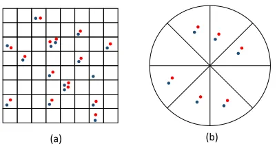
Fig. 2. Bucketing Schemes used for uniform correspondence sampling (a) Rectangular grid (b) Polar grid
et al [1] introduced the idea of bucketing to select feature correspondences to compute the fundamental matrix. The method involves dividing the image into ab×bgrid and then associating correspondences with each cell, see Figure 2. One correspondence is selected from eight randomly selected buck-ets which are sampled without replacement. In this process, a uniform random number generator is used to select a bucket in which the probability of selecting theithbucket is proportional to the number of correspondences lying within it. The sampled correspondences are used to instantiate a fundamental matrix from which the residuals of the remaining correspondences are computed. A statistical criterion based on the median is then used to determine the best candidate solution. This idea can be trivially extended to a spherical field of view camera by sampling from sectors of the circular image. Rituerto et al [18] consider bucketing in the context of feature track longevity in conventional perspective and omnidirectional field of view cameras. In the omnidirectional case the image is divided into a polar grid. They establish that the polar bucketing scheme allows for longer mean feature tracks in the context of a moving ground vehicle.
Miˇcuˇs´ık et al [19] present an algorithm to simultaneously estimate an omnidirectional camera model and epipolar ge-ometry from matching features. The accuracy of the computed camera model is a function of the distribution of features in the circular image. Namely, if features near the centre of the image are used the resulting model is incorrect. By rejecting these points and using the remaining matches the correct model can be found. This idea is effected through a bucketing technique which divides the image into concentric rings of equal area from which the algorithm then samples.
Along similar lines but different in implementation, Mei et al [20] suggested the idea of storing the features within a quadtree data structure in order to sample 2D features uniformly. The quadtree is a data structure which encodes the spatial relationship between the features. Strasdat [21] introduced an extension of this concept in the form of a depth first search to select features uniformly from the quadtree. Scaramuzza and Siegwart [22] present a visual odometry sys-tem for an outdoor vehicle utilising an omnidirectional camera. The system extracts SIFT features belonging to the ground plane in order to estimate the plane induced homography which is then decomposed into the rigid body motion. It is possible for the SIFT points to reside in only half of the
received circular image and the authors recognise that this yields an erroneous estimate using their standard algorithm. When the spatial distribution of features is evaluated to lie in half of the image, an alternative algorithm is used to estimate the motion.
To the authors’ knowledge no systematic analysis of the effect of spatial distribution on the accuracy of the computed rigid body transform has been performed. This is of practical relevance in the target application for several reasons. A non-uniform spatial distribution of 2D features may arise from cap-turing low texture images of generally homogeneous materials used in the construction of the pipework. In addition to this, blurred images may be acquired due to fast probe motion causing a reduction in feature matches - this is especially true for manual deployment. Omnidirectional lenses are often used in this application to capture a cross sectional view of the pipe surface in a single shot. However, the strong radial distortion of such lenses cause the appearance features to warp as they moves across the lens thus making the matching process more challenging - this warping leads to a reduction of feature matches. Hansen et al in [23] develop a version of SIFT to account for such radial distortion, however, the performance gains are negligible. Ultimately the estimated pose of the probe will be used to direct remedial action if any defects deemed to be a threat to safety are detected during the inspection. To this end, this article seeks to investigate this relationship under simple camera motion that is representative of the pipe mapping application. The paper proceeds by describing the simulation environment and the rationale behind the distributions, the analysis tools and results from running the simulation environment.
IV. SIMULATIONENVIRONMENT
A simulation environment was developed to consider the accuracy of relative camera pose computed from two spherical images as a function of feature coverage around the images and the number of noise corrupted correspondences used in the calculation. In accordance with the target application, the 3D points originate from a cylindrical surface. Correspondences were swept fromFminup toFmaxin steps of sizeFstepwhile coverage was varied by generating sectors of angle, S, from
0◦ up to 360◦ according to two coverage patterns described below. For a given Fstep, the sector angle, S, adhered to the
following constraint:
S≥ 360
Fstep
(4)
[image:3.612.75.276.58.166.2](a) (b)
Fig. 3. Example of coverage patterns for two sectors (a) Contiguous (b)
Equiangular
1𝑇2
𝑧
𝑥
𝑦 𝐹𝐶1
𝑧
𝑥
𝑦 𝐹𝐶2
𝑧
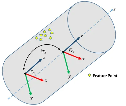
Fig. 4. Simulation of two cameras in a pipe with relative pose,c1Tc
2. The
3D points lie upon the surface of the pipe
was of interest, therefore, this constraint was relaxed. Note that the five point algorithm was found to be numerically unstable in some cases, therefore, the eight point algorithm was used instead. As a result, 8 matches were required as a minimum such that Fmin = Fstep = 8. In cases where M was not a factor of the number of features to be distributed amongst the sectors, the remainder were inserted sequentially from the first sector.
Two classes of distribution pattern were considered with respect to the coverage pattern of feature correspondences in the image. Given a fixed sector angle S, the first case incrementally adds feature correspondences from 0 to jS
degrees where j ∈ 1. . .360
S to form a contiguous region
of the image this is shown in Figure 3(a). In the second case, as shown in Figure 3(b), the feature correspondences are added toj sectors equally separated by an angle of 360j −S. An alternative approach would be to divide the image into concentric rings in the manner of [19], however, this would result in matches being distributed around 360◦ and thus restrict the non-uniform coverage aspect of the study. The feature correspondences were generated randomly and added to the sectors such that patterns with higher density included all points from a pattern with lower density. To prevent the final results being a function of specific feature correspondence patterns, the patterns were generated randomly and results averaged overN Monte Carlo trials.
The simulation made use of the forward and backward
projection functions,f(X)andg(X)obtained from calibrating a real camera with a fisheye lens [13] which was then used in the experimental validation of the study described in a section VIII. The camera had a resolution of 2048×2448 pixels and was calibrated to subpixel accuracy. The acquired image was a circle of radius 686 pixels with an inner circle of radius 180 pixels which contained no useful data as it pertained to the central black region of the pipe. The pose of the first camera,
wTc
1, was set to be parallel and positioned along the main axis of a pipe of radius 30 mm. Given knowledge of the field of view of the camera it was possible to compute the width,
W, of the observed cross sectional area when centred in the pipe. A second camera with pose,wTc2, was translated by
W
2
along the Z axis of the pipe relative to the first camera, thus forming the transform matrices:
wTc
1 =
1 0 0 0 0 1 0 0 0 0 1 0 0 0 0 1
,wTc2 =
1 0 0 0 0 1 0 0 0 0 1 W2 0 0 0 1
(5)
The constraint of translation only motion can be justified with reference to the target application where the camera will be approximately centralised in the pipe using circumferential brushes. Random 3D feature points were generated to lie within the region of intersection of the cameras view fields and spanned an angle defined by the sector size. For each camera, the 3D features were firstly transformed into the respective coordinate frame and then projected to form the image. A schematic of the setup is shown in Figure 4.
ciX=wT−1
ci
wX (6)
where wX ∈
R4×1 is a homogeneous vector of a point
on the surface of the pipe and g(ciX) is its projection in the image of camera ci. Through selection of the relative pose defined by Equation 5, the image points associated with each camera occupied 50% of the image. The image points corresponding to the second image were perturbed with additive white Gaussian noise of varianceσ2= 10pixels2 to simulate detector noise.
Using this simulation environment it was possible to gen-erate a controlled number of feature matches with known correspondence and varying coverage patterns. A summary of the input parameters, computed quantities and outputs of the simulation are shown in Table I.
V. ANALYSIS
[image:4.612.72.277.201.373.2]Simulation Input Input Parameter Computed Quantity Simulation Output
3D Point X F P
hCi,Fji
2D Point x 1Tˆ2 eF,Ct
Relative Pose 1T2 θF,C
Camera Model g(X),f(x)
Detector Noise σ2
Sector Size S
Feature Sweep F
Coverage Type Equiangular, Contiguous
TABLE I
SUMMARY OFSIMULATIONPARAMETERS
evaluated in terms of uncertainty, translation error and angular error, each error metric is discussed in turn.
The worst case configuration consisted of a single sector populated with the minimum number of correspondences. A comparison metric for uncertainty was used to express all other coverage and correspondence configurations relative to this case. Using the Monte Carlo approach, covariance matrices were generated from the expectation of vectors representing pose with the following form:
ˆ
p= [ˆqx,qˆy,qˆz,tˆθ,ˆtφ]T (7)
where the rotation, Rˆ, of the estimated transformation was converted into a unit length quaternion [25], qˆ. Note that the hat operator,ˆ, is used to denote an estimated quantity. The axis of rotation, [ ˆqx,qˆy,qˆz]T, was then extracted and
concatenated with the estimated direction vector expressed in spherical coordinates as azimuth and elevation angles θ and
φ respectively. The axis angle encoding of rotation provided by the unit quaternions and the use of spherical coordinates allowed a minimal problem representation.
In order to compare the covariance resulting from different coverage and correspondence configurations, a metric was required for measuring the distances between these matrices. Metrics such as the Jensen-Bregman LogDet divergence have been proposed in [26] in the context of image feature descrip-tors while [27] describe an approach based on the complex Wishart distribution in the application of synthetic aperture radar. In a similar manner to [24], Entropy measured in bits was used to express the relative magnitude of the uncertainty of the worst case coverage and correspondence configuration against all other configurations. Entropy is defined as follows:
En(i,j)=
1 2log2
det(P
hCi,Fji)
det(P
hC1,F1i)
(8)
where, P
hC,Fi ∈ R5×5, is a covariance matrix in which,
C, is the coverage index, F, is the feature count index and
detis the determinant operator. Geometrically, entropy can be considered to be a ratio of covariance ellipsoid volumes.
Given knowledge of the fixed true transformation, 1T 2, the
absolute error in rotation and translation were computed to give meaningful metrics with respect to the target application. For simplicity, they were computed separately rather than as a combined error metric. The estimated translation vectors,ˆt, resulting from N Monte Carlo trials are of unit magnitude due to the scaleless nature of monocular systems. In order to compare them with the true motion of the camera, the
estimated translation vectors were scaled by the magnitude of the true translation, |ttrue|, as follows:
ˆ
tscaled=ˆt|ttrue| (9)
such that the scaled translation error was in the unit of mm and thus meaningful in the pipe mapping context. The error was then calculated as the Root Mean Square Error (RMSE) in the XY plane:
e(tF,C)=
v u u t
1
N N
X
u=0
(ˆxu+ ˆyu)2 (10)
The rotation error was computed by forming the following matrix:
e
R=RRˆT (11)
which in the ideal case would be the identity matrix due to rotation being orthonormal. This was then mapped onto a scalar value [28] as follows:
θ(F,C)= cos−1(
tr(Re)−1
2 ) (12)
wheretr()is the trace operator.
It would be expected that each error metric would reduce for increasing correspondence count and coverage for both the contiguous and equiangular cases. Notwithstanding, it is the rate of reduction caused by the different coverage patterns that is of interest within this study. The following section presents results obtained from executing Monte Carlo trials of the simulation environment.
VI. RESULTS
0 -20
16 -15
16.7 32
-10
Entropy (bits)
-5
33.3
Match Count 48 0
Coverage %
50.0 66.7 83.3100.0 96 8064
(a)
0 0
1
16 2
3
16.7 32
RMSE (mm)
4 5
33.3
Match Count
48 6
Coverage %
50.0 66.7 83.3100.0 96 8064
(b)
0 0
0.02
16 0.04
0.06
16.7 32
Angular Error (
°)
0.08 0.1
33.3
Match Count
48 0.12
Coverage %
50.0 66.7 83.3100.0 96 8064
[image:6.612.57.288.67.277.2](c)
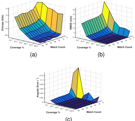
Fig. 5. Equiangular (a) Entropy for equiangular coverage (b) RMSE for
equiangular coverage (c) Rotational error for equiangular coverage
0 -20
16 -15
16.7 32
-10
Entropy (bits)
-5
33.3
Match Count 48 0
Coverage %
50.0 66.7 83.3100.0 96 8064
(a)
0 0
1
16 2
3
16.7 32
RMSE (mm)
4 5
33.3
Match Count
48 6
Coverage %
50.0 66.7 83.3100.0 96 8064
(b)
0 0
0.02
16 0.04
0.06
16.7 32
Angular Error (
°)
0.08 0.1
33.3
Match Count
48 0.12
Coverage %
50.0 66.7 83.3100.0 96 8064
(c)
Fig. 6. Contiguous (a) Entropy for contiguous coverage (b) RMSE for
contiguous coverage (c) Rotational error for contiguous coverage
values for 16.7% and 100% coverage when sweeping through the correspondence count. This was achieved by fixing the seed of the random number generator which allowed for easier comparison of error metrics. The detector noise variance was set to 0.1 pixels2 whileN = 500trials were run to compute a mean value for each performance metric. It was expected that the equiangular coverage pattern would result in lower uncer-tainty and lower estimation error of translation and rotation in comparison to contiguous coverage. This supposition is borne out by the previously defined metrics.
A. Entropy
The uncertainty in pose, expressed as entropy, is shown in Figure 5 (a) for the equiangular case and in Figure 6
(a) for the contiguous case. In both graphs it is evident that increased coverage causes entropy reduction as expected. However, for the equiangular case, the curve descends and plateaus at around≈ −20 bits with a coverage angle of 50% while the contiguous curve converges to a similar value at a greater coverage angle of 83.3%. Is is clear that the rate of reduction in the entropy-coverage projection of Figures 5 (a) and 6 (a) is greater than that for the rate due to correspondence increase. This demonstrates that the coverage of feature correspondences is more important beyond a certain number of matches,M, in this simulationM ≥16. As in [24] a continuous function of the form:
En(C, F) =a1log(C+a2) +a3log(F+a4) +a5; (13)
could be used to model the surface generated from the discrete points of the simulation assuming the large values along the minimum match count line of the graphs are discounted.
B. Translation
As shown in Figures 5 (b) and 6 (b), the maximum error was 6.4 mm which coincided with the fewest correspondences and least coverage. As expected, the minimum error was achieved at full coverage and matches with a value of 0.031 mm. For the equiangular case, at a coverage of 33% of the image circle, the RMSE was 0.034 mm while the contiguous coverage assumed an error of 0.195 mm. Thus with only 2 sectors separated by an angle of135◦ the error dramatically reduces to within approximately 12% of the final value achieved at full coverage and correspondence count. Only at a contiguous coverage of 83.3%, does the RMSE reduce to a comparable mean value of 0.036 mm. Note that the mean has been evaluated along the feature count axis forM ≥16. For both coverage patterns an increase in correspondences results in very little change in the RMSE in terms of the RMSE-No of Matches projection when
M ≥16.
C. Rotation Error
Interestingly, the estimate of rotation appears to be much less affected by coverage pattern in comparison to the trans-lation error and entropy. This agrees with the results of Rodehorst et al [29] in which relative pose algorithms are evaluated for multi-camera setups. They establish that for all tested algorithms, the estimate of camera rotation is much more stable than translation. As shown in Figures 5 (c) and 6 (c), the introduction of two sectors leads to a substantial reduction in error for coverage patterns. The coverage patterns converge to a final mean value of 9.15×10⁻⁶◦. At 50% coverage, the equiangular graph has essentially converged to the minimum value while for the contiguous case the rotation error has essentially converged to the final value at 83.3% coverage. Again beyond, M ≥ 16, for the Angular Error-Coverage projection the curves exhibit very little variability.
VII. DISCUSSION
[image:6.612.56.289.325.533.2]𝑑 𝑒
𝑒 Image 1
[image:7.612.106.244.56.170.2]𝑥1 𝑥2
Fig. 7. Illustrative 2D example of concept
to contiguous coverage thus demonstrating that greater uni-formity in coverage yields more accurate estimates of pose. The error in rotation has been shown to be less affected by the coverage pattern type, however, the equiangular case converges to in effect the final value at a quicker rate than contiguous coverage. Interestingly, beyond a minimum number of correspondences,M ≥16, the rate of reduction effectively plateaus for both patterns and coverage dominates.
The results may be explained through the simplified illus-trative example shown in Figure 7. In this diagram, image 2 is rotated with respect to image 1 around the midpoint,(0,0), of the image and two feature points, x1 andx2, disturbed by
noise, e, and separated by a distance, d, are used to compute the angle of this rotation. In the worst case the noise could result in the features assuming the values,x1+eandx2−e,
which would cause an angular error, θerror, of:
θerror= arctan(2e
d) (14)
By increasingd,θerror→0, for a fixed value ofe. Although simplified, this planar example serves to highlight the under-lying cause for the reduction in error caused by more uniform coverage in the image. The following section describes how the results of the simulation could be applied to a real world image sequence.
VIII. EXPERIMENTALVALIDATION
In order to demonstrate the use of the simulated results on real world data, an image sequence was acquired in an environment representative of the target application. A Point Grey Research Blackfly 2 camera with a fisheye lens producing an image circle of diameter 686 pixels was used for data collection. A ring of camera mounted LED’s was used to generate approximately uniform lighting inside a stainless steel pipe sample. The modelsg(X)andf(x)resulting from calibration [13] were used to produce the simulation error surfaces. Images were captured in discrete 10 mm steps (delivered by a KUKA KR5 robot) along a distance of 150 mm of the central axis of the pipe, see Figure 8 for the experimental setup. This allowed controlled steps between successive images with no motion induced image blur. This step size corresponded to approximately 50%overlap in the images, in practice this would be the minimum desired overlap. Because the simulation is evaluated on a finite grid, all combinations of coverage and feature correspondence counts
Fig. 8. Experimental Setup. Point Grey Research Blackfly camera mounted to KUKA KR5 for controlled linear motion
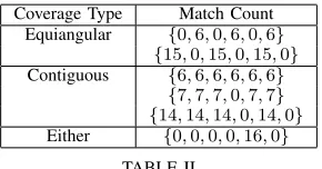
Coverage Type Match Count
Equiangular {0,6,0,6,0,6}
{15,0,15,0,15,0}
Contiguous {6,6,6,6,6,6}
{7,7,7,0,7,7} {14,14,14,0,14,0}
Either {0,0,0,0,16,0}
TABLE II
COVERAGEPATTERNENUMERATIONS
are not represented. The results of the simulation could be mapped onto a real world setting in the following manner. Given the feature correspondences extracted in a real image, all possible coverage patterns that are represented in the sim-ulation data could be enumerated. The error corresponding to the nearest neighbour within the simulation could then be used to estimate the expected error in the computed transform. The alternative would be to fit a function to the simulation surfaces that would map coverage and feature count to expected error in the transform as described in VI.
A predefined sector size of S = 60◦ was chosen for the experiment resulting in a six sector mask being applied to the raw images. The number of correspondences in each sector was then counted - an example is shown in Figure 10. Prior to counting the number of matches, some basic filters were used to reject gross outliers. The first filter removed correspondences in which the line connecting matching fea-tures crossed the inner circle of the image. The second filter removed matches where the length of the line,L, connecting matches satisfied the following constraint:
L > R2−R1 (15)
The filtered matches were subsequently used in a Random Sample Consensus [30] scheme to estimate the fundamental matrix and ultimately camera pose as described by Equations 1 - 3.
Given the match counts in the image of Figure 10, c =
{15,14,15,6,16,7} it was possible to enumerate the Equian-gular and Contiguous coverage patterns shown in Table II, some examples are shown visually in Figure 9.
[image:7.612.366.511.230.306.2](a) (b)
Fig. 9. Example of enumerated coverage patterns (a) Equiangular (b)
[image:8.612.322.547.59.397.2]Contiguous
Fig. 10. An example image acquired inside the pipe segment. Polar bucketing is applied followed by counting the number of correspondence in each sector.
count step, s, was computed as follows:
n=round(ci
s) (16)
where ci is the ith element of c. Assuming the noise level
contained in the simulation data is representative of the real world noise level, it could be used in the manner of a lookup table to place an upper bound on the expected transform error where the lookup table is essentially a form of the graphs shown in Figures 5 and 6 (b). A noise variance of
0.1 pixels2 was used to represent detector noise. Through
artificially masking out correspondences in post processing, it was possible to control coverage thus allowing the same dataset to be used to test the approach with different coverage patterns. Clearly, with pipes composed from different materials the distribution and number of correspondences will change however the algorithm is still applicable since the simulation data is independent of the imaged surface.
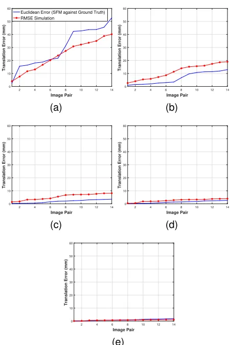
The true and predicted cumulative RMSE in translation for different coverage patterns consisting of 33%, 50%, 83% and 100% are shown in Figure 11. It can be seen that the simulation data for 33% and 100% under estimates the error while in the remaining cases, the error is over estimated. This is due to using the nearest neighbour approach to generate the simulation curves. Note that images were processed using visual odometry leading to an increasing error with increasing image pair. The error expressed as the difference between the final values of the curves for each of the graphs in Figure 11 was 12.61 mm, 6.05 mm, 4.59 mm, 1.31 mm and 0.79 mm respectively. In each graph, with the exception of Figure 11(a) the curves due to the simulation can be seen to follow
2 4 6 8 10 12 14
Image Pair 0
10 20 30 40 50 60
Translation Error (mm)
Euclidean Error (SFM against Ground Truth) RMSE Simulation
(a)
2 4 6 8 10 12 14
Image Pair
0 10 20 30 40 50 60
Translation Error (mm)
(b)
2 4 6 8 10 12 14
Image Pair
0 10 20 30 40 50 60
Translation Error (mm)
(c)
2 4 6 8 10 12 14
Image Pair
0 10 20 30 40 50 60
Translation Error (mm)
(d)
2 4 6 8 10 12 14
Image Pair
0 10 20 30 40 50 60
Translation Error (mm)
(e)
Fig. 11. Real error computed from known robot motion vs the predicted error from the simulation for different percentage coverages (a) 33.3% (b) 50% (c) 66.6% (d) 83.3% (e) 100%
the general trend of the error curve computed with respect to the robots motion.
The presented method allows an error to be estimated based purely upon the spatial distribution and number of matches which can be potentially fed into a Bayesian framework for an overall estimate of pose uncertainty. Furthermore, this operation can be performed at low computational cost since it only involves indexing a lookup table. In context of pipe mapping, this enables one to predict the error per metre travelled through the pipework which is invaluable knowledge with respect to remedial action.
IX. CONCLUSION
[image:8.612.118.231.217.331.2]which forms part of a visual pipe mapping sensor. In partic-ular, a quantitative measure of error and uncertainty on the estimation of a rigid body transform caused by non-uniform 2D feature correspondence coverage and a variable number of correspondences, perturbed by fixed pixel noise has been investigated. Sampling the matches through bucketing is often employed to mitigate bias and uncertainty in the computed camera pose, however this may not always be possible. This is true in the application of pipe mapping in which image features may be clustered due to prominent structures such as welds on an otherwise largely uniform texture surface. In such cases, the investigation presented here enables an error to be predicted from the percentage coverage of the matches and the number of such matches. It has been established through the development of a simulation environment, that the equi-angular coverage pattern results in more accurate estimates of pose in comparison to the contiguous case. A method has been developed to apply the results of the simulation to a real world example through using the simulation data as a lookup table. In the target application, the described method enables predictions with respect to the error incurred per metre travelled to be computed thus providing invaluable data for informing follow up remedial action.
ACKNOWLEDGMENT
This work was funded by Innovate UK (102067) in the ”Mo-saicing for Automated Pipe Scanning” project. The authors would like to thanks the project partners, National Nuclear Laboratory, Wideblue, Inspectahire and Sellafield Ltd.
REFERENCES
[1] Z. Zhang, R. Deriche, O. Faugeras, and Q.-T. Luong, “A robust technique for matching two uncalibrated images through the recovery of the
unknown epipolar geometry,” Artificial intelligence, vol. 78, no. 1,
pp. 87–119, 1995.
[2] C. N. Macleod, G. Dobie, S. G. Pierce, R. Summan, and M. Morozov, “Machining-based coverage path planning for automated structural
in-spection,”IEEE Transactions on Automation Science and Engineering,
vol. PP, no. 99, pp. 1–12, 2016.
[3] C. N. MacLeod, R. Summan, G. Dobie, and S. G. Pierce, “Quantifying and improving laser range data when scanning industrial materials,”
IEEE Sensors Journal, vol. 16, pp. 7999–8009, Nov 2016.
[4] R. Hartley and A. Zisserman,Multiple view geometry in computer vision.
Cambridge university press, 2003.
[5] R. Mur-Artal, J. Montiel, and J. D. Tardos, “Orb-slam: a versatile
and accurate monocular slam system,”Robotics, IEEE Transactions on,
vol. 31, no. 5, pp. 1147–1163, 2015.
[6] J. Kannala, S. S. Brandt, and J. Heikkil¨a, “Measuring and modelling
sewer pipes from video,” Machine Vision and Applications, vol. 19,
no. 2, pp. 73–83, 2008.
[7] P. Hansen, H. Alismail, P. Rander, and B. Browning, “Pipe mapping
with monocular fisheye imagery,” in Intelligent Robots and Systems
(IROS), 2013 IEEE/RSJ International Conference on, pp. 5180–5185, IEEE, 2013.
[8] K. Matsui, A. Yamashita, and T. Kaneko, “3-d shape measurement of pipe by range finder constructed with directional laser and
omni-directional camera,” in Robotics and Automation (ICRA), 2010 IEEE
International Conference on, pp. 2537–2542, IEEE, 2010.
[9] S. El Kahi, D. Asmar, A. Fakih, J. Nieto, and E. Nebot, “A vison-based
system for mapping the inside of a pipe,” inRobotics and Biomimetics
(ROBIO), 2011 IEEE International Conference on, pp. 2605–2611, IEEE, 2011.
[10] G. Dobie, R. Summan, C. MacLeod, and S. G. Pierce, “Visual odometry
and image mosaicing for nde,”NDT & E International, vol. 57, pp. 17–
25, 2013.
[11] D. G. Lowe, “Object recognition from local scale-invariant features,” in
Computer vision, 1999. The proceedings of the seventh IEEE interna-tional conference on, vol. 2, pp. 1150–1157, Ieee, 1999.
[12] P. Corke, Robotics, vision and control: fundamental algorithms in
MATLAB, vol. 73. Springer Science & Business Media, 2011. [13] D. Scaramuzza, A. Martinelli, and R. Siegwart, “A toolbox for easily
calibrating omnidirectional cameras,” inIntelligent Robots and Systems,
2006 IEEE/RSJ International Conference on, pp. 5695–5701, IEEE, 2006.
[14] D. Nist´er, “An efficient solution to the five-point relative pose problem,”
Pattern Analysis and Machine Intelligence, IEEE Transactions on, vol. 26, no. 6, pp. 756–770, 2004.
[15] R. I. Hartley, “In defense of the eight-point algorithm,”Pattern Analysis
and Machine Intelligence, IEEE Transactions on, vol. 19, no. 6, pp. 580– 593, 1997.
[16] G. Csurka, C. Zeller, Z. Zhang, and O. D. Faugeras, “Characterizing
the uncertainty of the fundamental matrix,”Computer vision and image
understanding, vol. 68, no. 1, pp. 18–36, 1997.
[17] T. Papadopoulo and M. I. Lourakis, “Estimating the jacobian of the
singular value decomposition: Theory and applications,” in Computer
Vision-ECCV 2000, pp. 554–570, Springer, 2000.
[18] A. Rituerto, L. Puig, and J. Guerrero, “Comparison of omnidirectional
and conventional monocular systems for visual slam,”10th OMNIVIS
with RSS, 2010.
[19] B. Miˇcuˇs´ık and T. Pajdla, “Omnidirectional camera model and epipolar
geometry estimation by ransac with bucketing?,” in Image Analysis,
pp. 83–90, Springer, 2003.
[20] C. Mei, G. Sibley, M. Cummins, P. Newman, and I. Reid, “Rslam: A
system for large-scale mapping in constant-time using stereo,”
Interna-tional journal of computer vision, vol. 94, no. 2, pp. 198–214, 2011.
[21] H. Strasdat,Local accuracy and global consistency for efficient visual
slam. PhD thesis, Citeseer, 2012.
[22] D. Scaramuzza and R. Siegwart, “Appearance-guided monocular
om-nidirectional visual odometry for outdoor ground vehicles,” Robotics,
IEEE Transactions on, vol. 24, no. 5, pp. 1015–1026, 2008.
[23] P. Hansen, P. Corke, W. Boles, and K. Daniilidis, “Scale invariant feature
matching with wide angle images,” inIntelligent Robots and Systems,
2007. IROS 2007. IEEE/RSJ International Conference on, pp. 1689– 1694, IEEE, 2007.
[24] H. Strasdat, J. M. Montiel, and A. J. Davison, “Visual slam: why filter?,”
Image and Vision Computing, vol. 30, no. 2, pp. 65–77, 2012. [25] J. Kuipers, “Quaternions and rotation sequences: A primer with
appli-cations to orbits, aerospace and virtual reality (p. 400),” 2002. [26] A. Cherian, S. Sra, A. Banerjee, and N. Papanikolopoulos, “Efficient
similarity search for covariance matrices via the jensen-bregman logdet
divergence,” in Computer Vision (ICCV), 2011 IEEE International
Conference on, pp. 2399–2406, IEEE, 2011.
[27] J. Schou, H. Skriver, A. A. Nielsen, and K. Conradsen, “Cfar edge
detector for polarimetric sar images,”IEEE Transactions on Geoscience
and Remote Sensing, vol. 41, no. 1, pp. 20–32, 2003.
[28] “E2919-14 standard test method for evaluating the performance of systems that measure static, six degrees of freedom (6dof), pose.” [29] V. Rodehorst, M. Heinrichs, and O. Hellwich, “Evaluation of
rela-tive pose estimation methods for multi-camera setups,” International
Archives of Photogrammetry and Remote Sensing (ISPRS08), pp. 135– 140, 2008.
[30] M. A. Fischler and R. C. Bolles, “Random sample consensus: a paradigm for model fitting with applications to image analysis and automated
cartography,”Communications of the ACM, vol. 24, no. 6, pp. 381–395,