QL-BT: Enhancing Behaviour Tree Design and Implementation with Q-Learning

City, University of London Institutional Repository

Citation

:

Child, C. H. T. and Dey, R. (2013). QL-BT: Enhancing Behaviour Tree Design

and Implementation with Q-Learning. Computational Intelligence in Games (CIG), 2013

IEEE Conference on, pp. 275-282. doi: 10.1109/CIG.2013.6633623

This is the unspecified version of the paper.

This version of the publication may differ from the final published

version.

Permanent repository link:

http://openaccess.city.ac.uk/3000/

Link to published version

:

http://dx.doi.org/10.1109/CIG.2013.6633623

Copyright and reuse:

City Research Online aims to make research

outputs of City, University of London available to a wider audience.

Copyright and Moral Rights remain with the author(s) and/or copyright

holders. URLs from City Research Online may be freely distributed and

linked to.

City Research Online: http://openaccess.city.ac.uk/ [email protected]

QL-BT: Enhancing Behaviour Tree Design and

Implementation with Q-Learning

Rahul Dey

[email protected]

Dr. Chris Child

[email protected]

Abstract— Artificial intelligence has become an increasingly important aspect of computer game technology, as designers attempt to deliver engaging experiences for players by creating characters with behavioural realism to match advances in graphics and physics. Recently, behaviour trees have come to the forefront of games AI technology, providing a more intuitive approach than previous techniques such as hierarchical state machines, which often required complex data structures producing poorly structured code when scaled up. The design and creation of behaviour trees, however, requires experience and effort. This research introduces Q-learning behaviour trees (QL-BT), a method for the application of reinforcement learning to behaviour tree design. The technique facilitates AI designers’ use of behaviour trees by assisting them in identifying the most appropriate moment to execute each branch of AI logic, as well as providing an implementation that can be used to debug, analyse and optimize early behaviour tree prototypes. Initial experiments demonstrate that behaviour trees produced by the QL-BT algorithm effectively integrate RL, automate tree design, and are human-readable.

Keywords—behaviour tree; Q-Learning; reinforcement learning; virtual environments; computer games

I. INTRODUCTION

Behaviour trees (BTs) have come to the forefront of artificial intelligence (AI) in games since their introduction in the last decade [1], and have been utilized in a number of games, including Halo 2 [2], Driver [3], and Spore [4]. They provide an intuitive, human readable and scalable form of representation for the decision making logic of non-player characters (NPCs).

Initial design of a BT requires experience and effort on the part of a designer. A poorly designed tree can cause AI characters to exhibit strange behaviour, breaking the user’s sense of immersion. This paper presents Q-learning behaviour trees (QL-BTs), a method for the application of reinforcement learning (RL) to enhance BT design. The technique assists AI designers by identifying the most appropriate scenarios in which to execute behaviours. Learned knowledge is integrated into a resulting BT data structure.

Experimental results show that the method exhibits a number of advantages over standard BT design techniques including: simplified BT designs; reduced code duplication;

and a restructured tree which provides optimization, taking the utility values of each action into account.

II. BACKGROUND

A. Behaviour Trees

A BT is a data structure designed to be a more intuitive revision of a finite state machine (FSM). FSMs represent NPC behaviour as a group of states and a number of transitions between these states [5]. As the number of states increases the number of transitions between the states can grow exponentially referred to by Knafla as an “often intangible growing mess” [6].

The combinatorial explosion associated with the number of transitions in an FSM is often mitigated by using hierarchical finite state machines (HFSM) where behaviours are split into smaller tasks. HFSMs with high state counts will, nonetheless, require a large number of transitions, again becoming difficult to manage [7]. BTs are similar to HFSMs in that they construct a hierarchy of behaviours where higher level behaviours (e.g. Attack) can be composed of atomic lower level behaviours (e.g. Find Weapon, Aim and Fire Weapon).

On each update, a BT performs a depth-first traversal until a low level behaviour (represented by a leaf node) has either succeeded or is set to the “running” state [8]. Due to this traversal method, behaviours are usually placed from left to right in descending order of priority to ensure that important behaviours are visited before less significant ones. For example, fleeing from the danger of an incoming grenade should be of higher priority than talking to a team mate [9].

In the standard form, BTs are composed of nodes that either dictate tree traversal logic or execute behaviours. Behaviour nodes contain various status codes to indicate the current behaviour’s state (“success”, “fail” or “running”). Traversal logic nodes are called Composite behaviours where, depending on the results returned from one or more of their children, they can succeed or fail. The most common examples of traversal logic nodes are the Sequence and Selector nodes [8][10].

Sequence nodes evaluate each child node in order and will only succeed if all children execute their behaviours successfully, similar to an AND-node in AND-OR trees [8]. Selector nodes also evaluate each child node in order but will

succeed as soon as any child executes a behaviour successfully and will stop checking later child nodes, similar to OR-nodes.

Another node commonly used in BTs is the Condition node [10]. These are usually located as part of a Sequence node’s children and can be used to check the state of an agent or the environment. Early checks within a Sequence node can indicate whether any of the node’s children are likely to succeed or fail and inhibit later behaviours in the sequence from running. This is particularly useful if the behaviour to be executed is computationally expensive and the cost could be avoided. Condition nodes are the primary focus of this research.

B. Machine Learning and BTs

There has been some previous research applying machine learning techniques to BTs. There is currently, however, little research into automated manipulation or improvement of an initial BT implementation. Lim, Baumgarten and Colton [27] made use of evolutionary algorithms. They generated BTs by creating an initial population of trees and used genetic operators to produce improved BTs in the computer game DEFCON. Results of this research were marginally successful against the game’s AI players.

Perez et al. [11] have also applied evolutionary computing to BTs using a genetic programming approach based on grammatical evolution [13], where “the syntax of possible solutions is specified through a context-free grammar”. BTs were applied to procedurally generated levels in the game, Super Mario [14]. The research found that the initial grammar was too flexible for use with BT evolution and a modified version was applied using an AND-OR tree structure [8]. This structure, using alternating layers of Selector and Sequence nodes, is also recommended by Champandard [10] and was therefore considered appropriate for use with this research.

Case based reasoning (CBR) is the process of solving new problems based on prior experience [15]. Flórez-Puga et al. [16] applied CBR to BTs in order to dynamically retrieve behaviours from a knowledge base. The process requires the addition of querying functionality to the behaviour nodes, such that, an agent being in a particular state will cause the node to query the knowledge base for cases of similar states visited in the past, and load an appropriate behaviour. This method provided a further source of inspiration for QL-BTs. CBR techniques generate experiential records manually, whereas a similar method can be used to create knowledge in an automated manner, using RL.

A number of hybrid approaches to RL have been implemented, including hierarchical evolutionary learners [28] and, more relevant to games AI, evolving game controllers using RL [29]. Pena utilizes the WEREWoLF algorithm to combine evolutionary algorithms with RL with effective results [29]. BTs were used in the research but only as static behaviour for an opponent controller.

C. Q-Learning

Q-Learning [17] is an RL algorithm that creates and maintains a table of values which estimate the utility of taking an action in a state. The agent is given a function associating

states with a predetermined reward. The algorithm then feeds rewards back to state-action pairs that lead to reward states creating gradually improving utility estimates.

A state can consist of any configuration of variables in an environment. Q-learning is not a model based algorithm, however, and will only record a Q-value for a state that has been visited by the agent during training. Q-learning can also be applied as a perceptual model. For example, if percepts consisted solely of health values of agents, nothing would be learned regarding the positions of agents in the environment (which may in fact be an important factor).

The update formula for Q-learning is:

Q(s, a) = (1 - α)Q(s, a) + α(r + γ maxa’(Q(s', a' ) ) ) (1) Where:

 Q(s, a) is the Q value of the current state-action pair  Q(s’, a’) is the Q value of the successor state-action pair  r is the reward associated with the successor state  α is the learning rate parameter

 γ is the discount factor parameter

The learning rate parameter, α, determines the extent to which new information overrides the previous information in the Q value. The discount factor, γ, determines the importance of future versus immediate rewards [18].

Action selection for an agent is governed by a predefined policy such as greedy, ε-greedy or softmax [19]. A greedy policy will select the currently estimated best action at any time. An ε-greedy policy encourages exploration, over a purely greedy policy, by introducing a small probability of choosing any available action at random. This has the effect of balancing exploitation (choosing the best available action) and exploration of alternative actions. Experiments in this research used an ε-greedy policy, providing a flexible approach in the absence of domain information.

III. QL-BT:INTEGRATING Q-LEARNING INTO A BEHAVIOUR TREE

This section details the mapping of RL concepts to features of BTs used in QL-BTs. Q-learning systems are comprised of states, actions, and a reward function. Each agent’s internal state values were combined with percept values to provide a single state for use with the Q-learning algorithm.

A. Overview

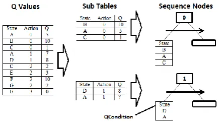
The algorithm begins with a BT as input. The tree is analysed to find the deepest Sequence nodes. These nodes are identified as actions for the RL stage. These actions are used in an offline Q-learning phase to generate a Q-value table. The table is then divided into sub-tables by action and the highest valued states for the action are extracted into the Q-Condition nodes within the BT. The Condition nodes in the input BT are then replaced with the Q-Condition nodes. Finally, the BT’s topology is reorganized by sorting each node’s child by their maximum Q-value, which provides AI designers with a more optimized permutation of the BT.

B. Generating Knowledge

The Q-learning algorithm is executed in a pre-processing step, generating experiential data that can be used in future runs of the simulation to determine the most appropriate action to execute in the agent’s current state. This inspired the replacement of Condition nodes with Q-Condition nodes: a simple lookup table containing all high-utility states, from which it was possible to select a particular action.

Tabular RL is used so that the Q-value table can be separated into sub-tables easily. The Q-values resulting from the initial Q-learning phase are divided into sub-tables for each action within the QL-BT. Each sub-table is then sorted in descending order of the Q value for each state. The states with the highest Q-values are extracted from the table, according to a parameter that determines the percentage of states to acquire. An example of the process can be seen in Figure 1. This example keeps all states for a particular action within the lookup tables. Later, the algorithm filters these by taking the top x percent of states in the tables (where x is a modifiable parameter).

C. Q-Condition Nodes

Q-Condition nodes contain a lookup table of high-utility states for a particular action. When these nodes are updated in the BT, a test is performed against the agent’s current state to check whether the state is present in the table. If present, the node passes, otherwise it fails.

Algorithm 1 shows the pseudo-code used to load Q-values from the initial Q-learning phase into the Q-Condition nodes. Rather than use standard Condition nodes that query the environment each time they are executed to establish whether an action can be performed (“Can I do this?”), Q-Condition nodes use knowledge acquired from the prior RL step to find out if an action should be performed (“Is this a good action based on what I already know?”).

For example, consider Figure 1. The Sequence node at the top of the image executes the behaviour “action 0” and the Q-Condition node contains “state A”. Let “action 0” be the Flee behaviour and “state A” mean “health is low”. The RL stage of the algorithm has determined that executing the Flee action from the low health state is desirable. This is the equivalent of a designer creating a Condition node testing whether an agent’s health is low. As the agent’s state updates whilst exploring the environment, instead of having to test using a manually created Condition node, it can look up its current state in a

Q-Condition node from a set of pre-evaluated states to determine whether it should execute a behaviour.

The required conditions for a behaviour to execute could also include tests that the designer has not previously considered. The designer can examine the highest utility states loaded into the Q-Condition nodes to find suggestions for conditions that could trigger behaviours.

D. Reorganizing Tree Topology

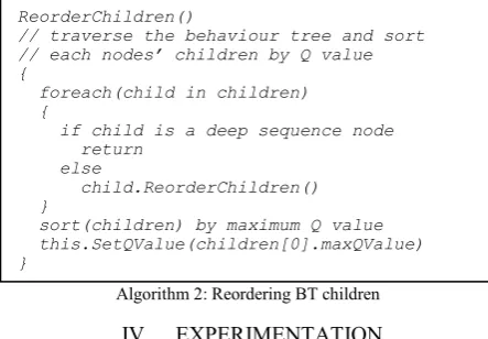
After the Q-Condition nodes have successfully loaded, the first element in the sorted array is the state exhibiting the highest Q-value when paired with the action (i.e. the maximum Q-value for the action). This maximum Q value is first stored in the Q-Condition’s parent node and can then be used to re-order the children. Algorithm 2, below, shows the ReorderChildren function, which recursively traverses the BT until it reaches one level above the deepest Sequence node. The children of the node reached are then sorted by their respective maximum values, in descending order, and the node’s Q-value is then set to the Q-Q-value of the first child.

Fig. 1: Inserting Q-values into QL-BT [] GetBestStates(action, pct, qvalues) // produces a sorted array of state-qvalue // pairs for an action

{

foreach(state in stateSpace) {

q = qvalues.GetQValue(state, action)

if(q > 0)

results.add(state, action, q) }

sort(results) by descending Q value numValues = results.size * (pct/100) return results[0]...results[numValues] }

Algorithm 2: Reordering BT children

IV. EXPERIMENTATION

The intention of this research was to assist designers by suggesting modifications to an input BT. It was therefore decided to use the most common application of BTs, a game scenario, to evaluate the performance of QL-BT. A simulation was created containing a group of prey and a group of predator agents. The prey’s reward function was designed to encourage behaviours which led to its survival. The input BT for each prey agent was also designed to have survival as their primary goal.

A. Agents

The predator agents made use of a simple finite state machine (FSM) [5], consisting of two states: Patrol and Attack. When prey agents were within a predator’s neighbourhood, the predator would transition from its Patrol to its Attack state where it selected one of the prey agents randomly and pursued it. If the predator killed the prey or lost track of it, it would transition back to the Patrol state where it would wander the environment randomly.

Both types of agents also made use of steering behaviours in order to move within the game world [30]. This allowed agents to move in a relatively free way without having to be constrained to paths.

100 prey agents and 20 predator agents were used in each experiment. Each prey agent had a finite set of actions that they could perform which were organised into a common BT (Figure 2).

The actions were defined as follows:

 Flee: Follow a steering vector away from the nearest predator agent

 SeekSafety: Move towards the nearest Haven zone (described below).

 Forage: Move towards the nearest Food zone (described below).

 Eat: When inside a Food zone, gain health each time this action is executed.

 Flock: Move according to location and orientation of neighbouring agents.

 Wander: Move towards a random point projected in front of the agent.

 Charge: Attack the nearest predator.

 Assist: Attack the nearest predator agent, targeting a neighbouring prey agent.

The initial BT consisted of a root Selector node that chose from three subtrees. The left most subtree (i.e. the highest priority branch) consisted of the “retreat” behaviours – Flee and SeekSafety. This was given the highest priority in order to try to ensure survival as a priority for prey agents.

The next subtree was the “idle” subtree, that was further split into two subtrees: “graze” (containing Forage and Eat behaviours); and “explore” (containing Wander and Flock behaviours). The “idle” subtree helps to define a prey agent’s natural behaviour when not under threat of attack.

The final subtree contained the “attack” behaviours. This subtree was placed at the lowest priority position in the BT as prey agents were intended to be non-combative but could defend themselves when necessary.

The predator-prey scenario incorporated inflicting damage to each agent so that more complex behaviours could be defined that extended beyond having a prey agent retreat from a predator every time. Each agent was given a health value of 100 and collisions between agents were resolved as follows:

 A predator in the Attack state colliding with a prey agent caused 7 units of damage to the prey agent.  A prey agent executing a Charge or Assist behaviour

colliding with a predator agent caused 5 units of damage to the predator agent.

 Predator-predator or prey-prey collisions caused no damage to either agent.

ReorderChildren()

// traverse the behaviour tree and sort

// each nodes’ children by Q value

{

foreach(child in children) {

if child is a deep sequence node return

else

child.ReorderChildren() }

sort(children) by maximum Q value this.SetQValue(children[0].maxQValue) }

B. Zones

The environment contained two types of zone in order to aid prey agents. These were Food zones and Haven zones.

Food zones simulated areas where prey agents could “eat” in order to regain health. Haven zones were areas that could not be entered by predator agents. These zones allowed the creation of interesting behaviour beyond simply fleeing from predators when they were seen.

C. Prey State and Rewards

Each prey agent was given a percept: a set of state values representing the agent’s perception of its environment. The percept was updated each frame of the simulation. The percept contained values for:

 Health (None, Low, Medium, High);

 Number of ally neighbours (None, Low, Medium, High);

 Distance to nearest Food (Inside, Near, Medium, Far);  Distance to nearest Haven (Inside, Near, Medium,

Far);

 Distance to nearest Predator (Inside, Near, Medium, Far).

Each value in the percept was divided into categories, such as none, low, medium and high, discretising environmental states. These were then combined into a single integer value that represented an index to the state space of the simulation.

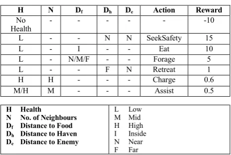
Rewards were administered using a predefined table that associated some state-action pairs with rewards. For example, when the agent’s health was depleted, any further action had a penalty of -10. If the agent had low health, was near a haven, was near an enemy, and then executed the SeekSafety action, it gained a reward of 15. Table 1 shows the full set of reward values. All other state-action pairs resulted in a reward of 0. These values were chosen after initial experimentation and observation of preliminary results.

In a computer game setting, it is desirable for agents to exhibit actions that appear intelligent from the perspective of a human observer. Rewards were therefore biased in favour of such behaviours. If, for example, an agent is being chased and is closer to a haven than a food source, it would be appropriate for the agent to travel to the haven.

D. Implementation and Visualisation

Three sets of simulations were each run 100 times, and the result of the trials recorded. At the beginning of each trial, both prey and predators’ positions were randomized within the confines of the game world. Each trial ended when either:

 All prey agents were within a Haven zone.  All prey agents were dead.

 All predator agents were dead.

 A timeout value was reached (set to 7500 ticks of the update loop).

TABLE 1:REWARDS FOR STATE-ACTION PAIRS

The first set of simulations used a standard BT for the prey AI. The second set used a greedy policy on the learned Q-values (always choosing the highest utility action from the current state). The third set used the BT containing Q-Condition nodes (QL-BT) instead of standard Condition nodes. Results at the end of each trial recorded:

 Number of living prey;

 Number of living prey that were safe (i.e. within a haven zone at the end of the trial);

 Average health of prey;  Number of living predators;  Average health of predators.

The Q-learning pre-processing stage ran for 1,000,000 iterations and the resulting values were stored. Both the learning rate (α) and the discount factor (γ) were set to 0.9, allowing agents to learn at a reasonable speed and providing a balance between maximizing current rewards and potential future rewards. An ε-greedy policy was used in order to promote exploration of the state-action space, with the ε parameter set to 0.3. No further learning was applied when each set of trials was run.

In the experimentation stage: the Q-learning prey agents employed a greedy policy on the previously learned Q-values in order to make decisions; and the QL-BT prey agents loaded the appropriate values into each Q-Condition node. The percentage of states loaded into each Q-Condition node was 50, resulting in half of the possible states observed for a particular action being loaded into each sub-table.

In some instances the agents would not perform any action because they were in a state that none of the Q-Condition nodes included, resulting in the tree traversal failing because all conditions would fail. Perez et al. [11] also noticed this when evolving BTs and resolved the issue by adding an unconditional fall-back behaviour. During the experiments, a similar mechanism was adopted, with the use of a fall-back branch that contained a RandomWalk action which always succeeded. This provided two advantages: first, the agent would convey the sense of some intelligence (the illusion of intelligence is particularly important to maintain player engagement in a game environment [12]); and second, the behaviour made the agent wander the environment updating its

H N Df Dh De Action Reward No

Health - - - -10

L - - N N SeekSafety 15

L - I - - Eat 10

L - N/M/F - - Forage 5

L - - F N Retreat 1

H H - - - Charge 0.6

M/H M - - - Assist 0.5

H Health

N No. of Neighbours Df Distance to Food

Dh Distance to Haven

De Distance to Enemy

state accordingly, thus being more likely to be in a state contained within one of the Q-Condition nodes.

V. EVALUATION

A. Reordered BT

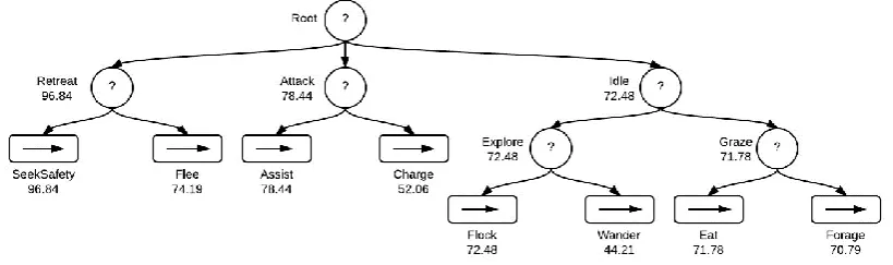
Figure 3 shows the reordered QL-BT after the Q-learning stage had taken place, in which some of the sub-trees of the original BT have been reorganized. Most notably, the Idle branch has been given the lowest priority by making it the last child of the root node. This indicates that the learning phase has found that the Wander and Flock behaviours are less useful in achieving the overall goal of survival for prey agents.

Another suggested reordering was within the Attack branch. The Assist behaviour had a higher maximum Q-value than the Charge which still supports the intended passivity of prey agents, while still able to defend other agents.

B. Number of Prey Alive

Table 2 shows that the majority of prey agents survived in each of the three trial types. Slightly fewer prey agents survived when using the Q-learning algorithm on its own, and the standard deviation indicated slightly more dispersion within the results, as can be seen in Figure 4. However, the standard deviations for the BT and the QL-BT trials were very similar and relatively small, indicating a stable set of values and providing an indication that the two BT types were performing similarly.

C. Number of Prey Safe

Table 3 shows the results for the number of prey in Haven areas at the end of each trial. Use of the standard BT resulted in some of the prey agents seeking safety. Both the relatively high standard deviation shown in the table and the trial results shown in the graph (Figure 5) show that the percentage of agents seeking safety varied widely between each trial execution .

When employing the Q-learning algorithm, a relatively small minority of the remaining prey agents resided within a haven zone. The percentage of safe prey was substantially lower (84.9% prey unsafe on average) than the results of the BT (60.2% prey unsafe on average).

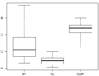
Promising results were demonstrated by the QL-BT. On average 47% of prey agents were within a Haven zone at the

end of each trial: almost twice as many as the mean number of prey using the BT alone, and almost half of the entire prey population. In addition, the standard deviation was substantially reduced, indicating the QL-BT outperformed the standard BT in this test.

D. Number of Predators Alive

Table 4, shows the number of living predator agents at the end of the simulation and provides interesting results. The prey agents using the original BT did not kill any predators in any of the trials. In stark contrast to this, however, when the prey used the greedy Q-learning algorithm they exhibited aggressive behaviour, resulting in almost all of the predators (~95% on average) being killed in each trial.

When using QL-BT, less than 5% of the predator population was killed on average. Use of the original BT resulted in all predators surviving every trial. The aggression shown by the Q-learning agents was substantially reduced in the QL-BT, which indicated attacking predator agents directly was implicitly discouraged, but necessary in some cases. These few cases could be inferred to demonstrate altruistic behaviour by prey agents defending their neighbouring flock mates. This conclusion is further supported by the reordered BT (Figure 3) in which the Assist action (attack a predator when a flockmate was being attacked) has a much higher Q value than the Charge action (attack the nearest predator).

TABLE 2: MEAN RESULTS FOR ALIVE/DEAD PREY

Simulation Type

BT QL BT with QL

Mean Alive Prey 84.41 79.13 86.5 Standard Deviation 3.44 5.33 3.52

TABLE 3: MEAN RESULTS FOR SAFE/UNSAFE PREY

Simulation Type

BT QL BT with QL

Mean Safe Prey 27.4 8.75 47 Standard Deviation 15.96 4.48 7.1

TABLE 4: MEAN RESULTS OF ALIVE/DEAD PREDATORS

Simulation Type

BT QL BT with QL

Mean Alive Predators 20 0.82 19.01 Standard Deviation 0 0.869 1.08

E. Discussion of Results

QL-BT agent attacked fewer predators during the test runs than Q-learning agents. This behaviour maintained the intended image of prey passivity, but also demonstrated altruism in appropriate situations.

BTs re-ordered using QL-BT demonstrated the use of prior knowledge in order to execute behaviours within Q-Condition nodes, instead of manually crafted Condition nodes, for each possible condition. This can reduce both the design and implementation time required for the tree allowing designers to

shift their focus from the creation of specific conditions to developing the behaviours of agents.

The tree reordering suggested an optimized BT that successfully prioritized behaviours by their respective utility values and ensured that all behaviours would be executed at the appropriate times. The resulting utility values could provide designers with an initial metric to determine the frequency of an executed action, which can be useful for debugging BTs when creating behaviours that are intended to run in many situations but are found to be executed rarely.

A drawback of the QL-BT algorithm is its reliance on correct Q-values. The validity of the Q-values relies on an appropriate reward function and an effective learning phase providing accurate utility estimates for each state-action pair. Values can be improved by a longer training period because this is an offline pre-processing step and does not cause performance issues at run-time.

Further drawbacks of Q-learning based techniques, in general, are that the simulation time for a complex game can be intractable, and the time taken to produce accurate Q-values is exponential to the state-action space of the agent. This research mitigated the problem by discretizing state values into a small number of categories using an agent’s perception of the state-space. However, additional research could further develop techniques for large state spaces.

QL-BT provides an advantage over the manual generation of prior cases presented in [16], in that the use of RL automates the generation of knowledge and stores it in the tree at runtime, providing a simple and intuitive process for designers to use.

The reordering of the BT at the end of the learning process is an optimization step that can suggest to designers the best tree-structure to use (as learned by the RL stage of the algorithm). These changes could signal errors at early stages of development (an important factor in reducing design and development time) and allow designers to choose which parts of the changed structure they incorporate into the final BT. Llansó et al. [21] demonstrate a method of validating BTs, however their findings are reliant on a component-based architecture to identify potential errors within a BT which requires domain knowledge on the part of the designer. QL-BT provides an approach which can be generalised more easily, requiring no domain-dependent tweaks, and can be applied to many different types of architectures and game engines. The learning approach is completely independent of the architecture of the game and the type of game being developed.

VI. CONCLUSIONS AND FUTURE WORK

This paper has presented Q-learning behaviour trees, a technique which combines RL with BTs. Results in a predator-prey scenario show that a tree resulting from QL-BT performs on a par with the original BT or outperforms it in all areas.

The state space of a typical game is, however, a concern if the technique is to be applied more generally. Combating the “curse of dimensionality” created by large state-spaces is an active area of research, and Approximate Dynamic Programming (ADP) [22] techniques could be applied to the Fig. 4: Boxplot showing number of prey alive in 100 trials

Fig. 5: Boxplot showing number of safe prey in 100 trials

state space of a game by effectively reducing the dimensions an agent needs to explore. Furthermore, soft state aggregation [23] could be used to share knowledge between similar states with learning applied to the aggregated state space.

Q-learning has many variants which could provide optimizations to the learning process. Dyna-Q [19] uses a model of the environment to assist learning and could be implemented in the system. “On policy” algorithms such as SARSA [19] could also be utilized within the framework.

BTs are hierarchical data structures, therefore hierarchical RL techniques [24] such as MAXQ [25] could be used as a further benchmark for the research.

The Q-learning implementation used in this research could be improved by dynamically altering the learning rate using McClain’s formula [26], for example.

In light of the results, it is believed that QL-BT provides a number of key benefits to existing BT design and implementation. In the scenario presented the QL-BT performed on a par with standard BTs in some situations, and better in other situations. An issue that remains to be addressed is the reduction and approximation of the state space, but the simple Q-learning approach shows promising results.

Designing effective AI is a difficult and error prone task for game developers when manually crafting conditions to decide when a behaviour should execute. Behaviour trees provide an intuitive interface with which to create robust NPC AI. Q-learning behaviour trees integrate well with existing technology and provide a promising basis for future research.

REFERENCES

[1] D. Isla, "Handling complexity in the Halo 2 AI" in Game Developer Conf., San Francisco, 2005

[2] Halo 2, [video game] USA: Bungie, Inc., 2004

[3] S. Ocio, “Adapting AI Behaviors To Players in Driver San Francisco” in The Eighth Annual AAAI Conf. on Artificial Intelligence and Interactive Digital Entertainment, Stanford, CA, 2012.

[4] C. Hecker, “My liner notes for spore/Spore Behavior Tree Docs”, n.d. [5] M. Buckland, “AI Game Programming by Example”. Wordware

Gazelle, Plano, Tex.; Lancaster, 2004.

[6] B. Knafla, “Data-Oriented Streams Spring Behavior Trees”, blog, 9 Jul. 2011; http://www.altdevblogaday.com/2011/07/09/data-oriented-behavior-tree-overview/

[7] I. Millington and J.D. Funge, “Artificial Intelligence for Games”. Morgan Kaufmann/Elsevier, Burlington, MA, 2009.

[8] A.J. Champandard, “Behavior Trees for Next-Gen Game AI”, blog, 28 Dec. 2008; http://aigamedev.com/insider/article/behavior-trees/ [9] A.J. Champandard, “The #fsmgate Scandal and What it Means for Your

AI Architecture”, blog, 28 Mar. 2012; http://aigamedev.com/open/editorial/fsmgate-scandal/

[10] A.J. Champandard, “Understanding the Second Generation of Behavior

Trees”, blog, 26 Feb. 2012;

http://aigamedev.com/insider/tutorial/second-generation-bt/

[11] D. Perez et al., “Evolving Behaviour Trees for the Mario AI Competition Using Grammatical Evolution”, in: Applications of Evolutionary Computation, Springer Berlin Heidelberg, Berlin, Heidelberg, 2011, pp. 123–132.

[12] A.J. Champandard, “Teaming Up with Halo’s AI: 42 Tricks to Assist

Your Game”, blog, 29 Oct. 2007;

http://aigamedev.com/open/review/halo-ai/

[13] M. O’Neill, C. Ryan, “Grammatical evolution?: evolutionary automatic programming in an arbitrary language”. Kluwer Academic Publishers, Boston, 2003

[14] Super Mario Bros., [video-game], Nintendo, Inc, 1985

[15] J.L. Kolodner, “An introduction to case-based reasoning”, Artificial Intelligence Review 6, 1992, pp. 3–34.

[16] G. Florez-Puga et al., “Dynamic Expansion of Behaviour Trees”in The Fourth Annual AAAI Conf. on Artificial Intelligence and Interactive Digital Entertainment, Stanford, CA, 2008

[17] C.J.C.H. Watkins, “Learning from Delayed Rewards”. Ph.D. dissertation, Cambridge University, 1989

[18] I. Millington, “Artificial intelligence for games”, Morgan Kaufmann Publishers, San Francisco, CA, 2006.

[19] R.S. Sutton, “Introduction to reinforcement learning”, MIT Press, Cambridge, Mass, 1998.

[20] D. Xiaoqin et al., “Applying hierarchical reinforcement learning to computer games” in the IEEE Symp. on Computational Intelligence and Games, 2009, pp. 929–932.

[21] D. Llanso et al., “Self-Validated Behaviour Trees through Reflective Components” in The Fifth Annual AAAI Conf. on Artificial Intelligence and Interactive Digital Entertainment, Stanford, CA, 2009

[22] W.B. Powell, “Approximate dynamic programming: solving the curses of dimensionality”, Wiley, Hoboken, N.J, 2011

[23] S. Singh et al., “Reinforcement learning with soft state aggregation”, 1995.

[24] A.G. Barto and S. Mahadevan, “Recent Advances in Hierarchical Reinforcement Learning” in Discrete Event Dynamic Systems 13, 2003, pp. 341–379

[25] T.G. Dietterich, “Hierarchical Reinforcement Learning with the MAXQ Value Function Decomposition”, J. Artif. Intell. Res. (JAIR) 13, 2000, pp. 227–303.

[26] J. O. McClain, “Dynamics of exponential smoothing with trend and seasonal terms”, Management Science 20, 1974, pp.1300-1304 [27] C. u Lim, R. Baumgarten, and S. Colton, “Evolving behaviour trees for

the commercial game defcon,” in EvoGAMES, 2010.

[28] M. Yoshikawa, T. Kihira, and H. Terai, “Q-learning based on hierarchical evolutionary mechanism,” WSEAS Transactions on Systems and Control, vol. 3, no. 3, pp. 219–228, 2008.

[29] L. Pena, S. Ossowski, J.M. Pena, S.M. Lucas, "Learning and evolving combat game controllers," in the IEEE Symp. on Computational Intelligence and Games, 2012, pp.195-202