City, University of London Institutional Repository
Citation
: Zu, Y. (2015). Consistent nonparametric specification tests for stochastic
volatility models based on the return distribution (15/02). London, UK: Department of Economics, City University London.This is the published version of the paper.
This version of the publication may differ from the final published
version.
Permanent repository link:
http://openaccess.city.ac.uk/12206/Link to published version
: 15/02
Copyright and reuse:
City Research Online aims to make research
outputs of City, University of London available to a wider audience.
Copyright and Moral Rights remain with the author(s) and/or copyright
holders. URLs from City Research Online may be freely distributed and
linked to.
City Research Online: http://openaccess.city.ac.uk/ [email protected]
Department of Economics
Consistent nonparametric specification tests for
stochastic volatility models based on the return
distribution
Yang Zu1
City University London
H. Peter Boswijk2
University of Amsterdam
Department of Economics Discussion Paper Series
No. 15/02
1 Corresponding author: Email: [email protected]. Department of Economics, City University London, Northampton Square, EC1V 0HB, London, United Kingdom. Telephone: +44 (0)20 7040 8619. Fax: +44 (0)20 7040 8580.
Consistent nonparametric specification tests for
stochastic volatility models based on the return
distribution
Yang Zu
1City University London
H. Peter Boswijk
2University of Amsterdam
April 29, 2015
1Email: [email protected]. Department of Economics, City University London,
Northamp-ton Square, EC1V 0HB, London, United Kingdom. Telephone: +44 (0)20 7040 8619. Fax: +44 (0)20 7040 8580.
2Email: [email protected]. Amsterdam School of Economics, University of Amsterdam,
Abstract
JEL Classification: C58, C12, C14.
1
Introduction
In this paper we consider specification tests for a class of parametric stochastic volatility models, given by
dYt=σtdBt,
dσ2t =b(σt2;θ)dt+a(σt2;θ)dWt,
(1)
where (Bt, Wt)t≥0 is a bivariate standard Brownian motion process, where b and a are
known functions, and where θ is an unknown parameter vector. The model is tested within a larger class of nonparametric stochastic volatility models
dYt=σtdBt, (2)
where (σt)t≥0 is a stochastic process satisfying certain regularity conditions. The model
(2) is nonparametric in the sense that there is no parametric structure specified for the volatility process. Model (1) is often used in financial econometrics to describe a logarithmic stock price process (Yt)t≥0, where (σt)t≥0 is an unobserved spot volatility
process. It includes popular models such as the Hull-White model, the Heston model and the GARCH diffusion model, which motivates the development of specification tests for this class of models.
Let Y be observed discretely at times ti =i∆, i= 0,1, . . . , n. Consider the re-scaled
∆-period return sequence
Xi =
1
√
∆(Yti−Yti−1) = 1
√
∆
Z ti
ti−1
σsdBs, i= 1, . . . , n. (3)
Let (Xi)ni=1 having a stationary density, denoted by q(x), and let q(x;θ) be its
spec-ification implied by the parametric model (1). In this paper we propose to test the specification (1) by comparing the estimated parametric return density to its nonpara-metrically estimated counterpart. Stated formally, we are testing
H0 :q(x) = q0(x)∈ {q(x;θ), θ∈Θ},
where Θ ⊆Rk is the parameter space, and define θ
0 to be the true parameter under the
null hypothesis: that is, it satisfies q(x;θ0) = q0(x).
detecting certain deviations in the functions{b(.;θ), a(.;θ)}1; however, tests constructed
this way would still be an important ”first check” because of its empirical significance in any structural modelling. The problem could be solved by defining test statistics based on the transition distribution of the observed returns, we discuss this issue in Section 7. To formulate the test statistic, one can compare either the density functions or the cumulative distribution functions. It is known from the literature that generally speaking, density-based tests are more sensitive to local deviations, whereas distribution-based tests are more sensitive to global deviations (see e.g. Eubank and LaRiccia (1992), Escanciano (2009) and A¨ıt-Sahalia, Fan, and Peng (2009)), we thus consider both in this paper.
A long-span asymptotic scheme is used in this paper. That is, we consider the asymp-totics whenn → ∞with fixed ∆. This is because model (1) is often used to describe price processes observed at relatively low frequencies (usually daily), prominent microstructure noise effects in prices observed at higher frequencies make the model unsuitable for such data. Throughout, we assume that (Xi)ni=1 is a stationary and ergodic sequence, and
that it is β-mixing with exponentially decaying coefficients. In Appendix A, checkable sufficient conditions for these properties to hold in the parametric model are given.
The stochastic volatility model we consider here is essentially a (partially observed) two dimensional diffusion process, so our test is related to the vast literature of nonpara-metric test for diffusion models, such as A¨ıt-Sahalia (1996), Hong and Li (2005), Corradi and Swanson (2005), Li (2007), Chen et al. (2008), A¨ıt-Sahalia et al. (2010), Kristensen (2011) and A¨ıt-Sahalia and Park (2012), among others. However, the unobservability of the volatility process in Model (1) makes the aforementioned research not applicable. Closely related to this paper is Corradi and Swanson (2011), who consider a conditional distribution based nonparametric test for stochastic volatility models. Other than the test statistics we consider are different from that of Corradi and Swanson, the model we consider is also different. Corradi and Swanson consider the stochastic volatility model where the observed series is assumed to be strictly stationary; while in our model we assume the observed return series (first difference of the observed series) to be station-ary and we allow the observed series to exhibit say unit-root type of dynamics. From a practical perspective, the stochastic volatility model considered in Corradi and Swanson in more appropriate to be used with interest rate data, where mean-reversion is often observed; while our model is more appropriate for equity and exchange rate price data, where unit-root behaviour is often observed. Zu (2015) analyzes an alternative approach to a similar testing problem, by comparing the nonparametric kernel deconvolution esti-mator of the volatility density with its parametric counterpart.
The structure of this paper is as follows. Sections 2 and 3 discuss nonparametric and parametric estimation of the return density and distribution functions, respectively.
Section 4 defines the test statistics, derives their asymptotic null distributions and consis-tency, and discusses using the bootstrap to approximate the null distribution. In section 5 Monte Carlo evidence for the size and power properties of the tests are given. In Section 6 we study an empirical application. Section 7 discusses possible extensions and con-cludes. Technical assumptions are collected in Appendix A. The proofs for the theorems are collected in Appendix B.
2
Nonparametric estimation
We now discuss the nonparametric estimation of density and distribution functions. In the nonparametric model (2), estimation of the stationary marginal return density and distribution functions is considered under the direct assumption that the sequence (Xi)ni=1
is stationary, ergodic and β-mixing with exponentially decaying coefficients.
To estimate q(x), the stationary return density function of (Xi)ni=1. Let hn be a
bandwidth,K(.) be a kernel function. It is well known that the density functionq(x) can be estimated by the kernel density estimator
ˆ
q(x) = 1
nhn n
X
i=1 K
x−Xi hn
.
Under appropriate conditions on the bandwidth parameter and the kernel function, the consistency and asymptotic distribution of the kernel density estimator are classical re-sults, we refer the readers to e.g. Pagan and Ullah (1999).
Denote the distribution function of the sequence (Xi)ni=1 to be Q(x). Letting I(.)
denote the indicator function, the distribution function Q(x) can be estimated by the empirical distribution function
ˆ
Q(x) = 1
n n
X
i=1
I(Xi 6x).
3
Parametric estimation
Given a parameterization{b(x;θ), a(x;θ)}, to obtain the parametric estimate of the func-tions q(x;θ) and Q(x;θ), we first need an estimate for the parameter vector, denoted as ˆ
θ, then evaluate the two functions given ˆθ.
On the one hand, parametric estimation of stochastic volatility model is by no means an easy task; substantial research efforts were devoted to it in the past decades. Here we first briefly review the existing methods and just assume we have a parametric estimator satisfying certain conditions. On the other hand, evaluating the two functions given ˆθ is also not trivial, because the density and distribution functions of the observed returns usually do not have closed-form expressions and one needs to resort to approximation methods to evaluate them.
3.1
Parametric estimation of stochastic volatility models
Many efforts have been devoted to the estimation of stochastic volatility models in the past decades. For a review, see e.g. Renault (2009). Here we do not confine to any particular parametric estimation method, but only give conditions that a parametric estimator should satisfy. We will need different assumptions for the density function based test and the distribution function based test. For the density function based test, we only need to assume the parametric estimator ˆθn is
√
n-consistent. We will also need the parametrization to be smooth.
(P1a) Under the null hypothesis,
|θˆ−θ0|=Op(n−1/2),
and q(x, θ) is Lipschitz in the parameter θ with the Lipschitz constant L(x) to be square integrable.
For the distribution function based test, however, stronger assumptions are needed — the estimator has to satisfy a certain first order asymptotic expansion, which will be a non-vanishing part of the asymptotic distribution. We also need the parameterization to be differentiable.
(P1b) Under the null hypothesis,
√
n(ˆθ−θ0) =
1
√
n n
X
i=1
ψθ0(Xi) +op(1),
withPθ0ψθ0 = 0 andPθ0kψθ0k
3.2
Approximating parametric density and distribution
func-tion
When no closed-form expressions for the density and distribution functions exist, we can in principle use an Euler scheme to simulate the process and hence evaluate intractable functionals of the process.
Given an estimate ˆθ, the parameterization b(., θ) and a(., θ), the observation interval ∆, and the objective variablesXi = √1∆
Rti
ti−1σsdBs, i= 1, . . . , n, to be approximated, we
first choose an integermas the steps to simulatewithinthe interval ∆, and another integer
M as the number of ∆-interval returns, such that we simulate the process Y with step sizeδ = ∆/mform×M steps. Then take first differences to getδ-returns, and aggregate and rescale over everym returns to getM simulated ∆-returns,Xi∗,i= 1, . . . , M. Using a kernel density estimator we can approximate q(x; ˆθ) from the simulated sample with
q∗(x; ˆθ) = 1
M hM M
X
i=1 K
x−Xi∗ hM
,
where K(.) is a kernel function, andhM is the bandwidth parameter.
Standard consistency results for the kernel density estimator and convergence theo-rems for the Euler scheme simulation of stochastic differential equations imply that when
M → ∞, hM →0 and m → ∞, q∗(x; ˆθ) → q(x; ˆθ) pointwise in x ∈R. The convergence
should be understood as in the probability space of Monte Carlo simulation. For the tech-nical conditions on the kernel functionK(.), bandwidthhM and the consistency result for
the kernel density estimator, we refer to, e.g. Section 2.6.2 of Pagan and Ullah (1999). For the convergence result of the Euler simulation method, we refer to Chapter 9 of Kloeden and Platen (1992). The accuracy of this approximation is determined by the number M
and mthat we choose. Because these numbers do not have to be bounded by the sample size n, they can be chosen very large to make the approximation error arbitrarily small. The parametric distribution function ˆQ(x,θˆ) can be approximated analogously using the empirical distribution function with the simulated data. In this reason, in the following we take the approximated q∗(x;θ) and Q∗(x;θ) to be equal to the corresponding exact ones q(x;θ) and Q(x;θ) to avoid complication.
order to evaluate the conditional distribution given a certain value. However, we remark that for the purpose of conditional distribution function approximation given a certain value, simulating paths conditional on that value is not necessary.
Remark 2 Bhardwaj, Corradi, and Swanson (2008) notice that the Milestein scheme simulation for the stochastic volatility is not convergent if the commutative condition is not satisfied, which is the case for most of the stochastic volatility models with leverage effects. They use a generalized Milestein scheme from Kloeden and Platen (1992) to deal with this problem. We emphasize that the Euler’s scheme is valid both in univariate and multivariate diffusions, and it is convergent both in the weak and in the strong sense when the simulating interval goes to 0. When used with stochastic volatility model, usually the Eulers Scheme is applied to a finer grid within the needed sampling interval, as in the method used in this paper. This will not cause the “stochastic integral” problem as discussed in Bhardwaj, Corradi, and Swanson (2008). Actually the Euler’s scheme is widely used in the literature to simulate stochastic volatility models with leverage effects. This include Andersen and Lund (1997), Bollerslev and Zhou (2002), A¨ıt-Sahalia and Kimmel (2007) and Barndorff-Nielsen, Hansen, Lunde, and Shephard (2008), to name just a few.
4
Test statistics and asymptotic properties
4.1
Asymptotic null distribution and the consistency
Define
T1 =nh1/2 Z
R
(ˆq(x)−Kh∗q(x; ˆθ))2dx,
whereKh∗q(x; ˆθ) =
R
RKh(x−y)q(y; ˆθ)dyis the convolution ofKh(x) = K(x/h)/hwith
q(x; ˆθ), the functionK(.) and bandwidth hare the same as used in the definition of ˆq(x). Using the convoluted return density in the formulation of the test statistic corrects the bias of the test statistic and deliver better asymptotic properties of the test statistic, we refer to Fan (1994) for a discussion of this issue in the general density test problem with
i.i.d. data.
Theorem 1 Under the null hypothesis, and if (SV0)–(SV5), (N1)–(N4), and (P1a) are satisfied, then
T1−h−1/2 Z
R
K2(u)du
d
−
→ N
0,2
Z
R
q02(x)dx Z
R
K(2)(v)2
dv
where K(2)(v) denote the convolution of the kernel function K with itself. Let
ˆ
σ2 = 2
n n
X
i=1
ˆ
q(Xi)
Z
R
K(2)(v)2dv,
which is a consistent estimator of the variance of the asymptotic distribution, then
T2 =
T1−h−1/2 R
RK
2(u)du
ˆ
σ
d
−
→N(0,1).
The test T1 is not pivotal as it depends on the unknown density q0(x). However the
corresponding studentized test T2 is pivotal.
A Cramer-von Mises type statistic can be formulated by comparing distribution esti-mates:
T3 =n Z
R
(Qb(x)−Q(x; ˆθn))2dQ(x; ˆθ).
Theorem 2 Under the null hypothesis, and if (SV0)–(SV5), (N2) and (P1b) are
satis-fied, then as n → ∞
T3
d
− →
Z
R
GQI(· ≤x)−GQψTθ0(·)
∂Q(x, θ)
∂θ |θ=θ0
2
dQ(x), (4)
where GQ is a Q-Brownian bridge indexed by F = {I(· ≤ x), x ∈ R} ∪ {ψθ(·)}, with
zero mean and the covariance function Γ(f, g) = limk→∞P∞i=1Cov(f(Xk), g(Xi)) with f, g∈ F.
The above limiting distribution ofT3is a functional of a Brownian bridge process, and
it depends on the model structure (thus not model-free) as well as the unknown parameter values. For this reasons, this limiting theorem cannot be used directly to define critical values of the test. We discuss the approximation method to obtain test critical values in the next Section 4.2.
We then look at the asymptotic power of these tests under fixed alternatives. To be specific, we consider
H1 :{q(x) =q1(x)=6 q(x;θ),∀θ∈Θ}.
We will need assumptions on the parametric estimator under the alternative model.
(P1a1) Under the alternative hypothesis H1,
|θˆ−θ∗|=Op(n−1/2),
Theorem 3 Assume Conditions (SV0)–(SV5) and Assumptions (N1)–(N4), and (P1a1) in Appendix A; let α∈(0,1) be a level of significance, and Z1−α be the 1−α quantile of
the standard normal distribution. Then under H1,
P
T1−h−1/2 Z
R
K2(u)du >ˆσZ1−α
→1,
and
P (T2 > Z1−α)→1.
For the distribution based test, we assume that under the alternative hypothesis the parametric estimator satisfy
(P1b1) Under the alternative hypothesisH1,
√
n(ˆθ−θ∗) = √1
n n
X
i=1
ψθ∗(Xi) +op(1),
with Pθ∗ψθ∗ = 0 and Pθ∗kψθ∗k2 < ∞, and Q(x;θ) is differentiable with respect to
θ.
Theorem 4 Under the null hypothesis, and if (SV0)–(SV5), (N2) and (P1b) are satis-fied; let α∈(0,1) be a level of significance, and c1−α be the 1−α quantile of the limiting
distribution in (4), then as n→ ∞,
P(T3 > c1−α)→1.
As with most nonparametric tests, both tests are consistent. That is, they can detect any fixed deviation to the true model as long as the sample size is sufficiently large.
4.2
Bootstrap null distribution
We use a parametric bootstrap procedure to approximate the distributions of the tests under the null hypothesis. Parametric bootstrap is also called model based bootstrap. As contrary to classical bootstrap, where one generate bootstrap samples by resampling the available dataset, parametric bootstrap involves generating bootstrap samples by first estimating a parametric model and then simulating data from the estimated parametric model (see Section 6.5 of Efron and Tibshirani (1994)). The dependence of the bootstrap sample on the original data is only through the estimated parameters. The parametric bootstrap is in particular useful in approximating the null distribution in a testing con-text because it always simulates data based on the null model: it will mimic the null model both under the null hypothesis and under the alternative hypothesis. In contrast, bootstrap procedures that do not exploit the model structures will usually mimic the data generating process (alternative model) under the alternative hypothesis. For example, in testing diffusion models, Corradi and Swanson (2011) use a block bootstrap procedure. Since the block bootstrap procedure mimics the data generating process under the al-ternative hypothesis, the bootstrapped statistic cannot reproduce the null distribution under a misspecified model, and they further define a re-centered test statistic to make the block bootstrap to work.
The parametric bootstrap procedure is as follows (use T1 as an example):
Step 1 Given a parametric estimate ˆθ, and step size ∆, simulaten (original sample size) discretely observed returns {Xi∗}n
i=1, which is called one bootstrap sample. Notice
this step has to be done using the method in Section 3.2 over a finer grid.
Step 2 With this bootstrap sample, compute the nonparametric estimator ˆq∗(x) and the parametric estimator ˆθ∗, then compute the test statistic T1∗ analogous to T1.
Step 3 Repeat step 1 and 2 B times to get a bootstrap sample T1∗1, . . . , T1∗B for the statisticT1.
WhenBis large, the empirical distribution ofT1∗1, . . . , T∗B
1 approximates the finite sample
null distribution.
Theoretical justification of the proposed parametric procedure is missing in this pa-per. This is a highly non-trivial problem, although it can probably be solved using the methodology developed in Fan (1994) and Andrews (1997). In absence of such results, we use extensive Monte Carlo simulations to study the power properties of the tests under various realistic scenarios and across different sample sizes in the next section.
5
Monte Carlo simulations
In this section, we study the finite sample performance of the density-based testsT1andT2
section to determine the null distribution of the test statistic. The empirical quantiles of the null distribution are used to determine the critical values. The cross-validation method (e. g. Wasserman (2004), Section 20.3) is used to determine the bandwidth, and we use the Gaussian kernel in all the nonparametric kernel density estimators. The GMM method of Meddahi (2002) is used to estimate the parametric model. The GMM method is less efficient than the likelihood based method, but it achieves a good compromise between the estimation efficiency and computation time. To save space, for all the simulated size and power, we only report the results at 5% significance level.2
5.1
Size of the tests
We simulate 1000 sample paths of daily observations (∆ = 1/252) from the Heston model,
dYt =σtdWt,
dσt2 = 5(0.1−σt2)dt+ 0.75pσ2
tdBt,
(5)
where the two Brownian motions W and B are independent. Within one day, 10 steps are simulated to reduce discretization error. We consider the sample sizes 1000, 2000 and 3000, roughly corresponds to 4 years, 8 years and 12 years of daily observations.
With the parameters and sample sizes, the test statistics T1,T2 and T3 are simulated
1000 times. The distribution of these realized test statistics are taken as the true distri-bution (except for the Monte Carlo errors). For each of the realized 1000 sample path, we obtain 5 bootstrap samples and compute their resulting test statisticsT1∗,T2∗ andT3∗. Aggregating them together across 1000 sample yields 5000 bootstrap statistics. Their sampling distribution is taken as the distribution of the bootstrap method.
Table 1 summarizes the simulated 5% level size of all the tests for the three sample sizes. The bootstrap test statistics seem to have a reasonable size property, especially when the sample size is large. For T1 and T3, the size property becomes better as the
sample size increases, though this is not the case for T2.
[Table 1 about here.]
5.2
Power of the tests
We study the power performance of the tests under four different sample sizes 500, 1000, 2000 and 3000, and we still use 1000 simulations. We take the Heston model (5) as the null hypothesis. We evaluate the power functions of the three test statistics under the
2The computations in this section are conducted with MatlabR 2012b on the Lisa computing cluster
three families of alternative models. Each family of models is indexed by τ, with τ = 0 corresponding to the null model (5).
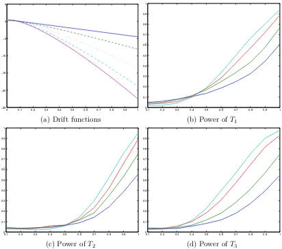
In the first family of alternative models, the drift functions of the volatility processes are deviated from the Heston model. In the second family of models, the diffusion func-tions are deviated from the Heston model. In the third family of models, jumps are included in the volatility process.
5.2.1 Misspecification in the drift function
We evaluate the power function of the three test statistics under the following sequence of alternative models,
dσ2t ={(1−τ)(α(β−σt2) +τ µ(σ2t)}dt+γpσ2
tdWt, (6)
for τ = 0,0.1, ...,1, where µ(σt2) = σt2[a(b−lnσ2t)] with a = 9, b = 3.5. The functional form of the drift part is motivated by the log SARV model
dYt = σtdBt,
d lnσt2 = κ(θ−lnσt2)dt+γdWt.
By Ito’s lemma, the volatility process of the log SARV model is
dσt2 =σt2
κ(θ−lnσ2t) + 1 2γ
2
dt+γσ2tdWt,
where the drift function is a highly nonlinear function of σ2
t and we use this to determine
the specification of µ(σ2
t).
Figure 1 shows the differences of the drift functions between the null model and the alternative models. It also gives the 5% level power functions of the three tests at the 4 different sample sizes. All the three tests show increasing power as the sample size goes large, confirming the consistency result of the tests. The performance of the three tests seems to be similar for this type of deviations in the drift function.
[Figure 1 about here.]
5.2.2 Misspecification in the diffusion function
process.
dYt =σtdBt,
dσt2 =α(β−σt2)dt+{(1−τ)γpσ2
t +τ ρ(σ
2
t)}dWt
(7)
for τ = 0,0.1, ...,1, where ρ(σ2
t) =cσ2t with c= 5. When τ = 1, the alternative model is
a GARCH diffusion process.
Figure 2 shows the differences of the diffusion functions between the null model and the alternative models. It also gives the 5% level power functions of the three tests at the 4 different sample sizes. Again all the three tests show increasing power (to 1) as the sample size goes large. The power of T1 seems to be slightly better than T3 when the
deviation is small, while when the deviation is large, the power seems to be similar. The power of T2 seems to be lower than the other two tests; when the sample size is small
(n= 500), the test T2 seems to have no power at all.
[Figure 2 about here.]
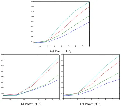
5.2.3 Jumps in the volatility process
We now consider the power of the three tests against a sequence of models where the volatility process contains jumps
dσt2 =α(β−σt2)dt+γpσ2
tdBt+Jt−dNt, (8)
where Nt is a Poisson process with intensity λ. Jt is the jump size that is independent
of (Wt) and (Bt). We consider the following 5 jump intensities: 52, 104, 252, 252×1.5,
252×2, these can be understood as the average number of jumps in a year. We consider a jump size that is normally distributed with mean 0 and standard deviation equal to 1.5%.
Figure 3 gives the power functions of the three tests under different sample sizes. We observe again the consistency of the three tests for this type of deviations to the null hypothesis. Also we see that as the jump intensity of the volatility process increases, the tests are more powerful in detecting the deviations. The relative performance of the three tests seems to be similar to this type of deviations.
[Figure 3 about here.]
6
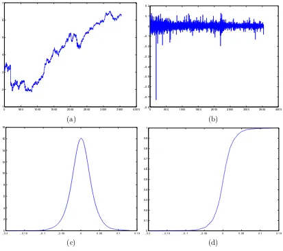
Empirical application
observations in total. Figure 4 gives the plot of the series, the log returns, the nonpara-metrically estimated density function, as well as the empirical distribution function of the dataset.
[Figure 4 about here.]
The dataset is fitted to the Heston model (5). The estimated parameter is ˆα = 17.5119, ˆβ = 0.1793, ˆγ = 2.4715. We then apply the nonparametric specification tests proposed in this paper to study the validity of the Heston model estimated. We still use the cross-validation method to determine the bandwidth and use the Gaussian kernel. Based on 1000 bootstrap samples, the estimatedp-values forT1,T2 andT3are 0.009, 0.014
and 0.000 respectively. Thep-values of all the tests provide strong evidence of rejection of the Heston model. The p-value of the distribution-based test is smaller than the p-values of the other two tests. From the Monte Carlo evidence, under the misspecification of the diffusion function, the distribution-based test seems to be slightly more powerful than the density-based tests. This give us the hint that the misspecification of the current model may come from the diffusion function. The results of this empirical application provides evidences that the model may not provide a good approximation of the marginal distribution of empirical data, although it is widely used in pricing options in real world applications.
7
Discussion and conclusion
We propose three tests for stochastic volatility model specification by comparing the parametrically and nonparametrically estimated stationary marginal density functions and distribution functions. Our approach can be adapted to discrete-time stochastic volatility models easily, as long as the volatility process is stationary. For example ,con-sider the classical discrete-time stochastic volatility model
yti = σtiεti,
logσt2
i = ω+γlogσ
2
ti−1 +σηηt,
(εt, ηt) ∼ i.i.d. N(0, I2).
When |γ| < 1, and the volatility process logσt2 is initiated from the stationary distri-bution N(ω/(1−γ), σ2
As discussed in the introduction section, the stationary marginal return distribution does not contain the information of dynamics in the data, such that tests defined on the marginal distribution will not be able to detect the misspecification in the dynamic structure of a model. To exploit the dependence structure in the model, we could consider to the one-step conditional distribution function and density function of Xi|Xi−1, i =
2, . . . , n, to formulate the test statistics.
Denote the density function of Xi|Xi−1 by p(y, x) and the corresponding conditional
distribution function by P(y, x).
For the nonparametric estimation of the two functions, we can proceed as follows. A simple kernel type density estimator forp(y, x) is
ˆ
p(y, x) =
1
nh2
n
Pn−1
i=1 K
x−Xi
hn
Ky−Xi+1 hn
1
nhn
Pn
i=1K
x−Xi
hn
,
and the estimator for the conditional distribution function P(y, x) is
ˆ
P(y, x) =
Pn−1
i=1 I(Xi 6x)I(Xi+16y)
Pn
i=1I(Xi 6x)
.
For parametric estimation of the above functions, we again need approximations and we can again resort to simulation based approximation.
Analogously to the univariate density based test, conditional density based test statis-tics can be formulated as:
T4 = Z
R2
ˆ
p(x, y)−Kh∗p(x, y; ˆθn)
2
dxdy,
whereKh(x, y) =K(x/h)×K(y/h)/h2 is the two dimensional kernel used in the definition
of ˆp(x, y). And the conditional distribution function based test is
T5 =n Z
R2
P(x, y; ˆθn)−Pˆ(x, y)
2
dP(x, y; ˆθn).
A similar parametric bootstrap is used to obtained the null distribution of the tests.
Appendix A: Basic setup and probabilistic properties
(N1) (kernel function) The kernel function K is a bounded, symmetric, nonnegative function on R, satisfying
Z ∞
−∞
K(x)dx= 1,
Z ∞
−∞
xK(x)dx= 0,
Z ∞
−∞
where k >0 is a constant, and
Z ∞
−∞
K2(x)dx <∞.
(N2) (density function)q(x) and its second order derivative are bounded and uniformly continuous on R.
The above assumptions on the kernel function, and the smoothness assumption on the density function are not the weakest possible. However, Assumptions (N1) and (N2) are sufficient for the present purpose and simplify the argument in the proof.
(N3) For the process (Xi)ni=1, all four dimensional joint densities of (yi1, . . . , yi1) exist, are
bounded and Lipschitz continuous. This implies that the corresponding distribution functions satisfy the same conditions.
(N4) As n → ∞,hn →0 and nhn → ∞.
These set of conditions will be used to derive the asymptotic properties of the test statis-tics, but together with the mixing conditions we assume throughout, they are also suffi-cient to make ˆq(x) a (pointwise) consistent estimator ofq(x) for allx∈R. (N3) is stronger than necessary for consistency, but will be required for the asymptotic distribution of the test based on the bivariate distribution of (Xi, Xi+1)ni=1−1.
The tests developed in this paper require the observed return sequence to be station-ary, ergodic andβ-mixing with exponentially decaying coefficients. In the nonparametric model, it is sufficient to assume the observed return sequence (Xi)ni=1 to satisfy the above
conditions directly. However, in the parametric model, it is non-trivial to check that these conditions are satisfied for particular choices of the functions b(x;θ) and a(x;θ). In the parametric stochastic volatility model (1), we first assume
(SV0) (B, W) is a standard Brownian motion in R2, defined on the probability space (Ω,F,P), and σ02 is random variable defined on the same probability space, inde-pendent of (B, W).
The following are standard assumptions from Genon-Catalot et al. (1998).
(SV1) For all θ ∈ Θ, the function b(x) = b(x;θ) is continuous on (0,+∞), and the function a(x) =a(x;θ) is continuously differentiable on (0,+∞), such that
∃K >0, ∀x >0, b2(x) +a2(x)≤K(1 +x2),
and
This assumption ensures the existence and uniqueness of an almost surely positive strong solution to the stochastic differential equation (1) generating the volatility process.
Define, for v0 >0, thescale measure
s(x;θ) = exp
−2
Z x
v0
b(v;θ)
a2(v;θ)dv
,
and thespeed measure
m(x;θ) = 1
a2(x;θ)s(x;θ).
Then the assumption
(SV2)
Z ·
0
s(x;θ)dx=∞,
Z ∞
·
s(x;θ)dx=∞,
Z ∞
0
m(x;θ)dx=M < ∞,
where the · in the integral means a arbitrary point in the domain of s(x;θ), ensures a unique and positive recurrent solution on (0,∞), see Genon-Catalot et al. (1998).
The last condition in (SV2) guarantees the existence of a stationary distribution (for the volatility process), with density defined as
π(x;θ) = m(x;θ)
M I(x >0).
If the process is initiated from this stationary distribution, i.e., under assumption
(SV3) The initial random variable σ02 has density π(x;θ), the solution is strictly stationary and ergodic.
Now we give sufficient conditions to ensure that the volatility process is β-mixing with exponentially decaying coefficients. From Theorem 3.6 of Chen et al. (2010), a sufficient condition (together with (SV1) and (SV2)) for exponential decay of theβ-mixing coefficients is that the process is ρ-mixing, so in the following we give the conditions for the process to beρ-mixing. Also, we note the result that if a diffusion process isρ-mixing, its ρ-mixing coefficients decay at an exponential rate (Bradley (2005), Theorem 3.3, or Genon-Catalot, Jeantheau, and Laredo (2000), Proposition 2.5). Furthermore, β-mixing andρ-mixing with exponential decay are almost equivalent concepts for scalar diffusions, as discussed in Chen et al. (2010).
(SV4)
lim
x↓0 a(x;θ)m(x;θ) = 0, xlim↑∞a(x;θ)m(x;θ) = 0.
(SV5) Let
γ(x;θ) =a0(x;θ)−2b(x;θ)
Appendix B: Lemmas and proofs
Conditions in Appendix A ensure strict stationarity, ergodicity and β-mixing of the volatility process. Notice that the return sequence (Xi)ni=1 is a sequence of stochastic
integrals of the volatility process with respect to an independent Brownian motion B
over small fixed intervals. By the following lemma from Zu (2015), the return series in-herit the stationarity, ergodicity and the β-mixing properties from the volatility process.
Lemma 1 In the model (1), if the volatility process (σt2)t≥0 is stationary, ergodic and β-mixing with a certain decay rate, then the normalized return sequence (Xi)ni=1 is also
stationary, ergodic and β-mixing, with a mixing decay rate at least as fast as that of
(σ2
t)t≥0.
In all the proofs in this appendix, we take the above mentioned probabilistic properties for the return series as given to avoid repetition. When we use a integral without the range of integration, the integration is over the full real axisR.
Proof (of Theorem 1) We first derive the asymptotic distribution of T1. Notice that
T1
= nh1/2 Z
(ˆq(x)−Kh ∗q(x; ˆθn))2dx
= nh1/2 Z
(ˆq(x)−Kh ∗q(x))2dx+nh1/2
Z
(Kh∗q(x)−Kh∗q(x; ˆθn))2dx
+nh1/2 Z
(ˆq(x)−Kh∗q(x))(Kh∗q(x)−Kh∗q(x; ˆθn))dx.
Define
T10 =nh1/2 Z
(ˆq(x)−Kh∗q(x))2dx.
It will be shown later that T10 = Op(1); the second term nh1/2
R
(Kh ∗ q(x) − Kh ∗ q(x; ˆθn))2dx=Op(h1/2) because ˆθn is a
√
n-consistent estimator forθ0 and the square
in-tegrable assumption on the Lipschitz constantL(x) as in Assumption (P1a), so this term is dominated by T10; the crossproduct term is clearly dominated by T10 by the Cauchy-Schuwarz inequality. Thus we have that
T1 =T10(1 +op(1)),
First notice
Z 1
n n
X
i=1
(Kh(x−Xi)−Kh∗q(x))
!2
dx
= 1
n2
n
X
i=1 Z
(Kh(x−Xi)−Kh∗q(x))2dx
+ 2
n2 X
i<j
Z
(Kh(x−Xi)−Kh ∗q(x))(Kh(x−Xj)−Kh∗q(x))dx
:= 1
n2
n
X
i=1
ϕn(Xi, Xi) +
2
n2 X
i<j
ϕn(Xi, Xj),
where
ϕn(u, v) :=
Z
(Kh(x−u)−Kh∗q(x))(Kh(x−v)−Kh ∗q(x))dx.
Next, we show that
1. The sum of the diagonal terms 1
n2
n
X
i=1
ϕn(Xi, Xi) p
−
→(nh)−1
Z
K2(u)du.
2. The sum of the off-diagonal terms
nh1/2 2 n2
X
i<j
ϕn(Xi, Xj)
!
d
− →N
0,2
Z
q02(u)du Z
(K(2)(u))2du
.
3. Then we show that
T10 −→d N
0,2
Z
q02(u)du Z
(K(2)(u))2du
,
Step 1 We first compute the order of the mean, E 1 n2 n X i=1
ϕn(Xi, Xi)
!
= 1
nEϕn(X1, X1)
= 1
n
Z Z
(Kh(x−X1)−Kh∗q(x))2dxq(X1)dX1
= 1
nh2
Z Z
K
x−X1 h
2
q(X1)dxdX1(1 +o(1))
= 1
nh
Z Z
(K(u))2q(X1)dudX1(1 +o(1))
= (nh)−1
Z
K2(u)du(1 +o(1)). (9)
Then we compute the order of the variance
Var 1
n2
n
X
i=1
ϕn(Xi, Xi)
!
6 E 1 n2
n
X
i=1
ϕn(Xi, Xi)
!2
= 1
n3Eϕ 2
n(X1, X1) +
2
n4 X
i<j
Eϕn(Xi, Xi)ϕn(Xj, Xj). (10)
We look at the two terms separately. For the first term
Eϕ2n(X1, X1)
=
Z Z
Kh2(x−X1)dx
2
q(X1)dX1(1 +o(1))
= 1
h4
Z Z
K2
x−X1 h
dx
2
q(X1)dX1(1 +o(1))
= 1
h2
Z Z
K2(u)du
2
q(X1)dX1(1 +o(1))
For the second term,
Eϕn(Xi, Xi)ϕn(Xj, Xj)
=
Z Z Z
Kh2(x−Xi)dx
Z
Kh2(x−Xj)dxq(Xi, Xj)dXidXj(1 +o(1))
= 1
h2
Z Z Z
K2(u)du
2
q(Xi, Xj)dXidXj(1 +o(1))
= O 1 h2 . (12)
Use the result in (11) and (12) in (10), we get
Var 1
n2
n
X
i=1
ϕn(Xi, Xi)
!
6 1 n3O
1
h2
+ 2
n4n 2O 1 h2 = O 1
n2h2
. (13)
Use the results in (9) and (13) and apply Markov’s inequality we have
P 1 n2 n X i=1
ϕn(Xi, Xi)−(nh)−1
Z
K2(u)du > ε ! 6 E n12
Pn
i=1ϕn(Xi, Xi)−(nh) −1R
K2(u)du 2 ε2 = O 1
n2h2
=o(1),
because nh→ ∞. Thus we have proved that
1
n2
n
X
i=1
ϕn(Xi, Xi)−(nh)−1
Z
K2(u)du = op(1).
Step 2 Now we use Theorem A, Appendix 1 in Hjellvik, Yao, and Tjøstheim (1998) to show
nh1/2 2 n2
X
i<j
ϕn(Xi, Xj)
!
d
− →N
0,2
Z
q02(u)du Z
(K(2)(u))2du
.
Notice that ϕn(x, y) is a degenerate symmetric kernel, and the mixing condition is
satis-fied.
the same distribution asXi. First we compute
Eϕ2n( ˜Xi,X˜j)
=
Z Z Z
Kh(x−Xi)Kh(x−Xj)dx
2
q(Xi)q(Xj)dXidXj(1 +o(1))
= 1
h2
Z Z Z
K(u)K
u+Xi−Xj
h
dx
2
q(Xi)q(Xj)dXidXj(1 +o(1))
= 1
h2
Z Z
K(2)
Xi−Xj h
2
q(Xi)q(Xj)dXidXj(1 +o(1))
= 1
h
Z Z
(K(2)(u))2q(Xj+uh)q(Xj)dudXj(1 +o(1))
= 1
h Z
(K(2)(u))2du Z
q2(x)dx(1 +o(1)).
then the asymptotic variance
σn2 = n
2
2 Eϕ
2
n( ˜Xi,X˜j) = n2
2h Z
(K(2)(u))2du Z
q2(x)dx(1 +o(1)). (14)
Then we check the conditions related to the 6 quantities Mni, i= 1, . . . ,6, as defined
in Theorem A, Appendix 1 in Hjellvik, Yao, and Tjøstheim (1998). ForMn1, notice that
for 1> δ >0,
E|ϕn(X1, Xj)ϕn(Xi, Xj)|1+δ
=
Z Z Z
Z
Kh(x−X1)Kh(x−Xj)dx
Z
Kh(x−Xi)Kh(x−Xj)dx
1+δ
q(X1, Xi, Xj)dX1dXidXj(1 +o(1))
=
Z Z Z
1 h4 Z K
x−X1 h
K
x−Xj h dx Z K
x−Xi h
K
x−Xj h dx 1+δ
q(X1, Xi, Xj)dX1dXidXj(1 +o(1))
=
Z Z Z
1
h2K (2)
X1−Xj h
K(2)
Xi−Xi h 1+δ
q(X1, Xi, Xj)dX1dXidXj(1 +o(1))
= h2
Z Z Z
1
h2K
(2)(u)K(2)(v)
1+δ
q(Xj +uh, Xj+vh, Xj)dudvdXj(1 +o(1))
= 1
h2δ
Z
|K(2)(u)|1+δdu
2Z
q(Xj +uh, Xj+vh, Xj)dXj(1 +o(1))
= O
1
h2δ
.
Using the same strategy it can be shown thatMn1 also has this upper bound and we thus
have
n2M 1 1+δ
n1 /σ2n=O
h h2δ/(1+δ)
=Oh11+−δδ
Similarly, we can show that
E|ϕn(X1, Xj)ϕn(Xi, Xj)|2(1+δ) = O
h2 h4(1+δ)
=O
1
h4δ+2
,
E|ϕn(X1, Xj)ϕn(Xi, Xj)|2 = O
1
h2
,
E|ϕn(X1, Xi)ϕn(Xj, Yk)|2(1+δ) = O
1
h4δ+2
,
which further imply that
n32M 1 2(1+δ) n2 /σ
2
n =O
1
n1/2hδ/(1+δ)
=o(1),
n32M 1 2 n3/σ
2
n=O
1
n1/2
=o(1).
n32M 1 2(1+δ) n4 /σ
2
n =O
1
n1/2hδ/(1+δ)
=o(1),
by noticing again that δ/(1 +δ)<1/2 and nh→ ∞. For Mn5, we first calculate
E Z
ϕn(X1, Xi)ϕn(X1, Xj)dP(X1)
2(1+δ)
= Z Z Z Z
Kh(x−X1)Kh(x−Xi)dx
Z
Kh(x−X1)Kh(x−Xj)dx
q(X1)dX1
2(1+δ)
q(Xi, Xj)dXidXj(1 +o(1))
= Z Z Z 1 h4 Z K
x−X1
h
K
x−Xi
h dx Z K
x−X1
h
K
x−Xj
h
dx
q(X1)dX1
2(1+δ)
q(Xi, Xj)dXidXj(1 +o(1))
= Z Z Z 1
h2K
(2)
X1−Xi
h
K(2)
X1−Xj
h
q(X1)dX1
2(1+δ)
q(Xi, Xj)dXidXj(1 +o(1))
= Z Z Z 1 hK
(2)(u)K(2)
u+Xi−Xj
h
q(Xi+uh)du
2(1+δ)
q(Xi, Xj)dXidXj(1 +o(1))
6 1
h2(1+δ)
Z Z Z
K(2)(u)K(2)
u+Xi−Xj
h
2(1+δ)
q(Xi+uh)duq(Xi, Xj)dXidXj(1 +o(1))
= h
h2(1+δ)
Z Z Z
|K(2)(u)K(2)(u+v)|2(1+δ)q(Xi+uh)duq(Xi, Xi−vh)dXidv(1 +o(1))
6 C× h
h2(1+δ)
Z
|K(2)(u)|2(1+δ)du
2
= O
1
h2δ+1
.
also have this upper bound andMn5 =O h21δ+1
. We thus have
n2M 1 2(1+δ) n5 /σ
2
n=O
h
h2(1+2δ+1δ)
=O
h2(1+1δ)
=o(1).
Similarly we have
E Z
ϕn(X1, Xi)ϕn(X1, Xj)dP(X1) 2 = O 1 h , and
n2M 1 2 n6/σ
2
n=O
h12
=o(1).
We have then checked the condition 1 σ2 n n2 M 1 1+δ
n1 +M 1 2(1+δ)
n5 +M
1 2 n6
, n32
M
1 2(1+δ)
n2 +M
1 2 n3+M
1 2(1+δ) n4
→0,
and the CLT for the U-statistic is proved and we have finished proving Step 2.
Step 3 The asymptotic distribution ofT10 is an easy consequence of Step 1 and 2. The asymptotic distribution of T1 is obtained by noticing T1 =T10(1 +op(1)).
For the asymptotic distribution of T2. First use the result in Fan and Ullah (1999)
Theorem 4.1 we have
1 n n X i=1 ˆ
q(Xi) p
− →
Z
q2(x)dx,
then the CLT for T2 follows easily from Slutsky’s lemma.
In proving Theorem 2, we will need the following weak convergence results for empir-ical process ofβ-mixing sequences:
Lemma 2 (Kosorok (2008), Theorem 11.24) Let X1, X2, . . . be stationary with marginal distribution P, and β-mixing with
∞ X
k=1
k2/(p−2)β(k)<∞,
for some 2 < p < ∞. Let F be a class of functions in L2(P) satisfying the entropy condition, where the bracketing number satisfies
J[ ](∞,F, Lp(P))<∞. (15)
then
Gnf =n1/2 n
X
i=1
(f(Xi)−P f) d
inl∞(F), wheref 7→GPf is a tight, mean zero Gaussian process with covariance function
Γ(f, g) = lim
k→∞ ∞ X
i=1
Cov(f(Xk), g(Xi)),
for all f, g ∈ F.
Proof (of Theorem 2) We prove the theorem using empirical processes techniques. We are working with dependent data, so we need the empirical process result for β-mixing sequences in Lemma 2, which is Theorem 11.24 in Kosorok (2008). The exponential decay of β-mixing coefficients is sufficient for the above lemma to work.
We first prove
√
n(Qb(x)−Q(x; ˆθn)) l
∞(F)
x7→GQI(u6x)−GQψθT0
∂Q(x, θ)
∂θ |θ=θ0, (16)
using the strategy discussed in Van der Vaart (2000), pp. 278–279. Here the notation
l∞ denote weak convergence of stochastic process. Notice that
√
n(Qb(x)−Q(x; ˆθn)) =
√
n(Qb(x)−Q(x;θ))−
√
n(Q(x; ˆθn)−Q(x;θ))
= √n(Qb(x)−Q(x;θ))−
√
n(ˆθn−θ)
∂Q(x, θ)
∂θ ,
= √n(Qb(x)−Q(x;θ))−
1 √ n n X i=1
ψθ(Xi)
∂Q(x, θ)
∂θ +op(1),
where we use the differentiability of the parameterization and the assumption (P1b) about the expansion of the parametric estimator. With this, the above limiting distribution is determined by the joint distribution of
√
n(Qb(x)−Q(x;θ)),
1 √ n n X i=1
ψθ0(Xi)
! .
Notice that our F is the class of indicator functions F = {I(−∞, x)}, which satisfies the entropy condition (15) and thus is a Donsker class. Adding the k components of ψθ
to F will make a larger class which we call G, which is again Donsker (a finite class is Donsker); this is because the union of Donsker classes is also Donsker. Therefore
√
n(Qb(x)−Q(x;θ)),
1 √ n n X i=1
ψθ0(Xi)
!
l∞(G)
g 7→GQg,
and using the continuous mapping theorem we get
√
n(Qb(x)−Q(x;θ))−
1 √ n n X i=1
ψθ0(Xi)
∂Q(x, θ)
∂θ
l∞
x7→GQI(u6x)−GQψθT
∂Q(x, θ)
Notice that the processGQI(u6x) and the variable GQψθT are dependent because they
can be viewed as marginals of the processg 7→GQg. Therefore, under the null hypothesis,
(16) is proved.
Then, under the null hypothesis,
T2n = n
Z
(Qb(x)−Q(x; ˆθn))2dQ(x; ˆθ)
=
Z √
n(Qb(x)−Q(x; ˆθn))
2
dQ(x;θ0)(1 +Op(n−1/2))
=
Z √
n(Qb(x)−Q(x; ˆθn))
2
dQ(x;θ)(1 +op(1)),
and the result of the theorem follows easily from continuous mapping, because the map
z 7→ R
z2(t)dQ(t) from D[−∞,+∞] into
R is continuous with respect to the supremum
norm.
Proof (of Theorem 3) Under the alternative hypothesis, we can make the following decomposition of the test statistic,
T1
= nh1/2 Z
(ˆq(x)−Kh∗q(x; ˆθn))2dx
= nh1/2 Z
(ˆq(x)−Kh∗q1(x))2dx+nh1/2 Z
(Kh∗q1(x)−Kh∗q(x; ˆθn))2dx
+2nh1/2 Z
(ˆq(x)−Kh∗q1(x))(Kh∗q1(x)−Kh∗q(x; ˆθn))dx
Using the same approach as in Theorem 1, it can be shown that the first term satisfies
nh1/2 Z
(ˆq(x)−Kh∗q1(x))2dx−(nh)−1 Z
K2(u)du
d
−
→ N
0,2
Z
q02(u)du Z
(K∗K)2(u)du
.
For the second term, by definition
Z
(Kh∗q1(x)−Kh ∗q(x; ˆθn))2dx p
− →
Z
(q1(x)−q(x; ˆθn))2dx=Op(1),
as h → 0, because this is the L2 distance between the alternative model and the
pe-sudotrue model. The limit exists because we are considering functions in the L2 space.
Thus we have
nh1/2 Z
For the third term, by Cauchy-Schuwarz inequality
Z
(ˆq(x)−Kh∗q1(x))(Kh∗q1(x)−Kh∗q(x; ˆθn))dx
6 Z
(ˆq(x)−Kh∗q1(x))2dx
1/2Z
(Kh∗q1(x)−Kh∗q(x; ˆθn))2dx
1/2
= Op(n−1/2h−1/4).
Then it is obvious that T1 → ∞ underH1 and the test is consistent.
The consistency of the test T2 can be shown analogously.
Proof (of Theorem 4) Let F(x) = Q(x, θ∗) be the projection of Q1(x) onto the space
of parametric models. That is, Q(x, θ∗) is the pseudotrue model. Let X1, X2, . . . be
the observations generated from Q(x, θ∗), and denote ˆF(x) be the empirical distribution function of the sample {Xi}ni=1. Then under the alternative hypothesis, we can make the
following decomposition
T3
= n Z
( ˆQ(x)−Q(x; ˆθn))2dQ(x; ˆθn)
= n Z
( ˆQ(x)−Fˆ(x))2dQ(x; ˆθn) +n
Z
( ˆF(x)−Q(x; ˆθn))2dQ(x; ˆθn)
+2n Z
( ˆQ(x)−Fˆ(x))( ˆF(x)−Q(x; ˆθn))ddQ(x; ˆθn).
When n → ∞, the first term
n Z
( ˆQ(x)−Fˆ(x))2dQ(x; ˆθn) p
− →n
Z
(Q1(x)−F(x))2dF(x) = Op(n).
Using the same method as in the proof of Theorem 2, it can be shown that the second term nR
( ˆF(x)−Q(x; ˆθn))2dQ(x; ˆθn) satisfy the same convergence in distribution result
as in that theorem, such that
n Z
( ˆF(x)−Q(x; ˆθn))2dQ(x; ˆθn) =Op(1).
By Cauchy-Schuwarz inequality the cross product term is Op(n1/2). Then it is obvious
References
A¨ıt-Sahalia, Y. (1996). Testing continuous-time models of the spot interest rate. Review of Financial Studies 9, 385–426.
A¨ıt-Sahalia, Y., J. Fan, and J. Jiang (2010). Nonparametric tests of the Markov hypoth-esis in continuous-time models. The Annals of Statistics 38(5), 3129–3163.
A¨ıt-Sahalia, Y., J. Fan, and H. Peng (2009). Nonparametric transition-based tests for jump diffusions. Journal of the American Statistical Association 104, 1102–1116. A¨ıt-Sahalia, Y., L. P. Hansen, and J. A. Scheinkman (2010). Operator methods for
continuous-time Markov processes. In Y. A¨ıt-Sahalia and L. P. Hansen (Eds.),
Hand-book of Financial Econometrics, Volume 1, pp. 1–66. Amsterdam: North Holland.
A¨ıt-Sahalia, Y. and R. Kimmel (2007). Maximum likelihood estimation of stochastic volatility models. Journal of Financial Economics 83(2), 413–452.
A¨ıt-Sahalia, Y. and J. Y. Park (2012). Stationarity-based specification tests for diffusions when the process is nonstationary. Journal of Econometrics 169(2), 279–292.
Andersen, T. and J. Lund (1997). Estimating continuous-time stochastic volatility models of the short-term interest rate. Journal of Econometrics 77(2), 343–377.
Andrews, D. W. (1997). A conditional Kolmogorov test. Econometrica: Journal of the
Econometric Society, 1097–1128.
Andrews, D. W. (2005). Higher-order improvements of the parametric bootstrap for markov processes. Identification and Inference for Econometric Models: Essays in
Honor of Thomas Rothenberg, Cambridge, 171–215.
Barndorff-Nielsen, O. E., P. R. Hansen, A. Lunde, and N. Shephard (2008). Designing realised kernels to measure the ex-post variation of equity prices in the presence of noise. Econometrica 76, 1481–1536.
Bhardwaj, G., V. Corradi, and N. R. Swanson (2008). A simulation-based specification test for diffusion processes. Journal of Business & Economic Statistics 26(2), 176–193. Bollerslev, T. and H. Zhou (2002). Estimating stochastic volatility diffusion using
condi-tional moments of integrated volatility. Journal of Econometrics 109, 33–65.
Bradley, R. C. (2005). Basic properties of strong mixing conditions. A survey and some open questions. Probability Surveys 2, 107–144.
Chen, S., J. Gao, and C. Tang (2008). A test for model specification of diffusion processes.
Annals of Statistics 36, 167–198.
Chen, X., L. P. Hansen, and M. Carrasco (2010). Nonlinearity and temporal dependence.
Journal of Econometrics 155, 155–169.
Corradi, V. and N. Swanson (2005). Bootstrap specification tests for diffusion processes.
Journal of Econometrics 124, 117–148.
304–324.
Efron, B. and R. J. Tibshirani (1994). An introduction to the bootstrap, Volume 57. CRC press.
Escanciano, J. C. (2009). On the lack of power of omnibus specification tests.Econometric
Theory 25(01), 162–194.
Eubank, R. and V. LaRiccia (1992). Asymptotic comparison of cramer-von mises and nonparametric function estimation techniques for testing goodness-of-fit. The Annals of Statistics, 2071–2086.
Fan, Y. (1994). Testing the goodness of fit of a parametric density function by kernel method. Econometric Theory 10, 316–356.
Fan, Y. (1995). Bootstrapping a consistent nonparametric goodness-of-fit test.
Econo-metric Reviews 14(3), 367–382.
Fan, Y. and A. Ullah (1999). On goodness-of-fit tests for weakly dependent processes using kernel method. Journal of Nonparametric Statistics 11, 337–360.
Franke, J., J.-P. Kreiss, and E. Mammen (2002). Bootstrap of kernel smoothing in nonlinear time series. Bernoulli 8(1), 1–37.
Gao, J. and I. Gijbels (2008). Bandwidth selection in nonparametric kernel testing.
Journal of the American Statistical Association 103, 1584–1594.
Gao, J. and M. King (2004). Adaptive testing in continuous-time diffusion models.
Econo-metric Theory 20, 844–882.
Genon-Catalot, V., T. Jeantheau, and C. Laredo (1998). Limit Theorems for Discretely Observed Stochastic Volatility Models. Bernoulli 4, 283–303.
Genon-Catalot, V., T. Jeantheau, and C. Laredo (2000). Stochastic volatility models as hidden Markov models and statistical applications. Bernoulli 6, 1051–1079.
Hjellvik, V., Q. Yao, and D. Tjøstheim (1998). Linearity testing using local polynomial approximation. Journal of Statistical Planning and Inference 68, 295–321.
Hong, Y. and H. Li (2005). Nonparametric specification testing for continuous-time mod-els with applications to term structure of interest rates.Review of Financial Studies 18, 37.
Kloeden, P. E. and E. Platen (1992). Numerical Solution of Stochastic Differential Equa-tions. Berlin: Springer.
Kosorok, M. R. (2008). Introduction to Empirical Processes and Semiparametric Infer-ence. Berlin: Springer.
Kristensen, D. (2011, October). Semi-nonparametric estimation and misspecification testing of diffusion models. Journal of Econometrics 164(2), 382–403.
Li, F. (2007). Testing the parametric specification of the diffusion function in a diffusion process. Econometric Theory 23(02), 221–250.
Pagan, A. and A. Ullah (1999). Nonparametric Econometrics. Cambridge: Cambridge University Press.
Pham, T. D. and L. T. Tran (1985). Some mixing properties of time series models.
Stochastic Processes and Their Applications 19, 297–303.
Renault, E. (2009). Moment-based estimation of stochastic volatility models. In T. G. Andersen, R. A. Davis, and J.-P. K. T. Mikosch (Eds.), Handbook of Financial Time Series, pp. 269–311. Berlin: Springer.
Van der Vaart, A. (2000). Asymptotic Statistics. Cambridge: Cambridge University Press.
Wasserman, L. (2004). All of statistics: a concise course in statistical inference. Springer. Zu, Y. (2015). Nonparametric specification tests for stochastic volatility models based
0 0.1 0.2 0.3 0.4 0.5 0.6 0.7 0.8 0.9 1 −25
−20 −15 −10 −5 0 5
(a) Drift functions
0.1 0.2 0.3 0.4 0.5 0.6 0.7 0.8 0.9 1
0 0.1 0.2 0.3 0.4 0.5 0.6 0.7 0.8 0.9 1
(b) Power of T1
0.1 0.2 0.3 0.4 0.5 0.6 0.7 0.8 0.9 1
0 0.1 0.2 0.3 0.4 0.5 0.6 0.7 0.8 0.9 1
(c) Power ofT2
0.1 0.2 0.3 0.4 0.5 0.6 0.7 0.8 0.9 1
0 0.1 0.2 0.3 0.4 0.5 0.6 0.7 0.8 0.9 1
[image:35.595.91.503.71.435.2](d) Power of T3
Figure 1: Power under the misspecification of the drift function. (a): drift function with
0 0.1 0.2 0.3 0.4 0.5 0.6 0.7 0.8 0.9 1 0
0.5 1 1.5 2 2.5 3 3.5 4 4.5 5
(a) Diffusion functions
0.1 0.2 0.3 0.4 0.5 0.6 0.7 0.8 0.9 1
0 0.1 0.2 0.3 0.4 0.5 0.6 0.7 0.8 0.9 1
(b) Power ofT1 under different sample sizes
0.1 0.2 0.3 0.4 0.5 0.6 0.7 0.8 0.9 1
0 0.1 0.2 0.3 0.4 0.5 0.6 0.7 0.8
(c) Power ofT2under different sample sizes
0.1 0.2 0.3 0.4 0.5 0.6 0.7 0.8 0.9 1
0 0.1 0.2 0.3 0.4 0.5 0.6 0.7 0.8 0.9 1
[image:36.595.89.504.71.435.2](d) Power ofT3 under different sample sizes
1 1.5 2 2.5 3 3.5 4 4.5 5 0
0.1 0.2 0.3 0.4 0.5 0.6 0.7 0.8 0.9
(a) Power of T1
1 1.5 2 2.5 3 3.5 4 4.5 5
0 0.1 0.2 0.3 0.4 0.5 0.6 0.7 0.8
(b) Power of T2
1 1.5 2 2.5 3 3.5 4 4.5 5
0 0.1 0.2 0.3 0.4 0.5 0.6 0.7 0.8
[image:37.595.89.508.70.435.2](c) Power ofT3
0 500 1000 1500 2000 2500 3000 3500 4000 1
2 3 4 5 6 7
(a)
0 500 1000 1500 2000 2500 3000 3500 4000 −0.8
−0.7 −0.6 −0.5 −0.4 −0.3 −0.2 −0.1 0 0.1 0.2
(b)
−0.20 −0.15 −0.1 −0.05 0 0.05 0.1 0.15 2
4 6 8 10 12 14 16 18
(c)
−0.20 −0.15 −0.1 −0.05 0 0.05 0.1 0.15 0.1
0.2 0.3 0.4 0.5 0.6 0.7 0.8 0.9 1
(d)
[image:38.595.90.503.72.438.2]T1 T2 T3 n= 1000 0.0277 0.0581 0.0377
n= 2000 0.0372 0.0363 0.0400
[image:39.595.200.394.71.132.2]n= 3000 0.0406 0.0564 0.0411