Allocation of tasks for reliability growth using multi-attribute utility

Allocation of tasks for reliability growth using multi-attribute

utility

K.J. Wilson

School of Mathematics and Statistics, Newcastle University, UK

J. Quigley

Department of Management Science, University of Strathclyde, UK

Abstract

In reliability growth models in particular, and project risk management more generally, improving the reliability of a system or product is limited by constraints on cost and time. There are many possible tasks which can be carried out to identify and design out weaknesses in the system under development. This paper considers the allocation problem: which subset of tasks to undertake. While the method is applicable to project risk management generally, the work has been motivated by reliability growth programmes. We utilise a model for reliability growth, based on an efficacy matrix, developed with engineering experts in the aerospace industry. We develop a general multi-attribute utility function based on targets for cost, time on test and system reliability. The optimal subset is identified by maximising the prior expected utility. We derive conditions on the model parameters for risk aversion and loss aversion based on observed properties of preference. We give conditions for multivariate risk aversion under the general form of the utility function. The method is illustrated using an example informed by work with aerospace organisations.

Keywords: utility theory, reliability growth, Bayesian experimental design, multivariate risk aversion, expert judgement

1

Introduction

Selecting a programme of activities optimal against multiple criteria is cognitively challenging and time consuming for decision makers but can be aided with appropriate decision support tools if preferences can be represented mathematically. In the development of large, complex products or systems, the system is analysed at various stages for potential design weaknesses and, once weaknesses have been identified, they are designed out. This improves the system’s reliability. Examples of tasks which are used to identify weaknesses are fault tree analysis, failure modes and effects analysis, test, analyse and fix (TAAF), load strength analysis, vibration testing, simulation studies and accelerated life testing [24].

The outcomes of these tasks will not be mutually exclusive: tasks may expose multiple weak-nesses and weakweak-nesses may be exposed by various tasks. There will typically be neither the budget nor the time to carry out all of the potential reliability tasks. Therefore engineers choose and se-quence a subset of tasks to improve the product’s reliability. This paper considers methods to select such a portfolio of reliability tasks.

seek to represent preference trade-offs rather than vagueness of decision makers. Multi-attribute utility has been used in a similar manner in the area of portfolio resource allocation [30, 14, 1] and the simplifying assumption of utility independence is identified as desirable to specify a utility function.

In the context of reliability growth [33, 28] developed a model which aimed to represent the process experienced by engineers. It explicitly considered all of the potential faults and tasks to identify them resulting in the use of an efficacy matrix. The efficacy of each task is assessed against each potential failure mode producing an efficacy matrix for each pairing to measure the conditional probability of exposing the failure mode given its presence in the design. Such a matrix could have uses across project risk management problems. Reliability improves as specific design weaknesses are identified and removed from the system. All of the parameters in the model can be elicited from observable quantities. We use this model as the basis to solve the decision problem of task allocation. [33] also considered task allocation and outlined an integer programming approach which minimised costs subject to constraints on expected reliability and time on test. The shortcoming of this approach is that it provides little sensitivity around the reliability and time targets: an allocation which just failed to meet the targets was unacceptable and an allocation which met the targets was equally desirable.

In this paper we propose a Bayesian solution to the task allocation problem; choosing the allocation which maximises the prior expectation of a utility function representing the engineers’ preferences over cost, reliability and time on test. A general utility function over these attributes, which utilises the idea of mutually utility independent hierarchies, will be developed. The form of this utility function will be adapted to satisfy observed properties of marginal preferences from decision makers in experiments. In particular, we develop conditional utility functions to represent risk averse preferences and loss averse preferences which satisfy the isolation effect. That is, preferences of individuals over lotteries generally discard elements that the lotteries have in common [19, 32].

We consider the impact of the form of the utility function on preferences over multiple attributes and give conditions for the individual risk averse and loss averse utilities to lead to multivariate risk aversion [29]. The resulting optimal allocation is more sensitive to small changes in expected reliability and time on test around the target values than the integer programming approach. This is the first time multi-attribute utility has been used for task allocation in reliability growth modelling.

The contribution of the paper takes two forms; a theoretical contribution on multi-attribute utility and a methodological contribution on reliability growth specifically and project risk man-agement more generally. In the first case, we consider for the first time the implications for multivariate preference behaviour by assuming utility independence within a mutually utility in-dependent hierarchy (MUIH). Proposition 4 shows that such structures are sufficiently flexible to represent multivariate risk aversion, risk neutrality and risk seeking behaviour. Proposition 3 shows that not all attributes within a MUIH are by necessity utility independent. The illustrative example quantifies the impact of assuming different preference behaviours of the decision maker within utility functions. The preferences of the decision maker over multiple attributes can result in different optimal allocations of reliability tasks. In the second case, we develop a methodol-ogy within a reliability growth framework which allows engineers to make decisions about which activities to undertake which explicitly considers trade-offs between the important attributes in their decision. The methodology captures varying preference behaviours and gives an analytically tractable solution to the decision problem. We indicate the generalisation of the methodology to similar decision problems in project risk management.

the paper and identify future work in Section 5.

2

An expert judgement informed reliability growth model

We adopt the approach developed in [33, 28]. In Section 2.1 we define the efficacy matrix, which is core to the reliability growth model. In Section 2.2 we derive the reliability assessment for a design prior to undertaking reliability tasks. In Section 2.3 we derive the updated reliability assessment following the outcome of a reliability task.

2.1

The efficacy matrix

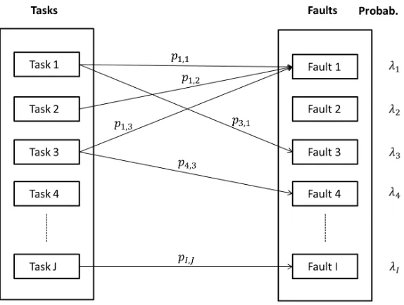
Suppose that the current design of an engineering system has associated with it a number of identified potential faults, labelledi= 1, . . . , I. Then, for each fault i, there is some probability, denotedλi, that this fault will be realized as a failure at some point in the lifetime of the system. DefineXi to be an indicator variable,

Xi=

(

1, if faultiis ever realised,

0, otherwise.

The probabilities ofXi being in its two possible states areλi and 1−λi respectively.

As part of the growth programme there are a number of possible tasks which could be performed on the system, labelled j= 1, . . . , J. Each task will have a certain efficacy at identifying each of the faults in the system. Denote bypi,j the conditional probability that taskj will realise faulti

given that the fault exists within the system.

An illustration of the efficacy matrix is given in Figure 1. We see the J possible tasks to identify theIpotential faults in the system. Each of the faults has an associated probability that it exists in the system. In the figure, task 1 will identify faults 1 and 3 with probabilitiesp3,1, p1,1

respectively. Fault 1 could also be identified by tasks 2 and 3. Therefore there are multiple routes which could identify fault 1. By contrast, none of the tasks in the figure can identify fault 2. The probability that fault 2 exists,λ2, will never change as a result of performing any task.

Figure 1: A diagram illustrating the form of the efficacy matrix

experts inside the organisation. For more information see [15]. Similarly, [35] developed a Bayesian model based on observable quantities for reliability growth in the TAAF cycle.

2.2

Prior reliability

Assume that each time a fault is found and removed no new fault is added to the system. Then in the system there will be some fixed unknown number of faults,N.

Assuming that the faults are independent then the reliability of the system at timetisR(t) =

QI

i=1Ri(t)Xi, whereRi(t) is the reliability associated with faulti at timet. Prior to performing

any tasks the expected reliability at timet[33] is

EX[R(t)] = I

Y

i=1

X

xi∈{0,1}

Pr(Xi=xi)Ri(t)xi_,

=

I

Y

i=1

[1−(1−Ri(t))λi].

That is, we can express the expected reliability of the system as a function of the reliability functions associated with each of the faults, which will typically be of a convenient parametric form, and the probabilities that each of the faults are present in the system.

2.3

Post-development reliability

Suppose we perform a number of the tasks. We either observe faultiin one of the tasks, di= 1, or not, di = 0. This will update, through Bayes Theorem, the probabilities of the faults truly existing to Pr(Xi = 1|di = 1) = 1, Pr(Xi = 0 | di = 1) = 0, as when a fault is found it must exist and

Pr(Xi=xi|di= 0) =

        

1−λi

1−λi[1−QJ

j=1(1−pi,j)θj]

, xi= 0,

λiQJ

j=1(1−pi,j)θj

1−λi[1−QJ

j=1(1−pi,j)θj]

, xi= 1,

whereθjis an indicator variable which takes the value 1 if taskj has been performed and 0 if not. The prior expectation of the reliability [33] is then

ED

EX|D[R(t)] = I Y i=1   X

di∈{0,1}

Pr(Di=di)

× X

xi∈{0,1}

Pr(Xi=xi|Di=di)Ri(t)I[xi>di]

  = I Y i=1 

1−(1−Ri(t))λi

J

Y

j=1

(1−pi,j)θj



,

where I[xi > di] is an indicator variable which takes the value 1 when xi > di and 0 otherwise. We see that we can evaluate the expected reliability of the system analytically once we know the reliability functions,Ri(t), associated with each of the faults.

3

The allocation of reliability tasks

3.1 we discuss some general characteristic of our multi-attribute utility function. In Sections 3.2 to 3.6 we explore the implications of loss averse and risk averse preferences of the decision maker.

3.1

General Bayesian solution

Each task will have associated with it a certain cost, denotedyj, and duration, denotedχj. Before a product can be released it needs to attain a specific target reliabilityR0. Any testing which is

undertaken is also subject to time restrictions given by the maximum total time on test χ0 and

cost restrictions given by the total budget for the testingY0. There may also be a target time on

testT0< χ0.

The total cost and total time on test following a set of tasks are given by

Y =

J

X

j=1

yjθj, χ=

J

X

j=1

χjθj,

respectively.

The objective of the design problem is to identify a subset of tasks which lead to a system with high reliability, low costs and low time on test.

The general Bayesian solution to this allocation problem is

max

θ1,...,θj∈{0,1}J

ED

EX|D[U(R, Y, χ)] ,

where U(R, Y, χ) is the utility function. That is, we maximise the prior expectation, over all of the possible subsets of tasks, of a utility function which represents the engineer’s preferences over the attributes in the problem, namely, reliability, cost and time on test.

Suppose that a decision maker was asked to specify their preferences over lotteries [11] which associate consequences (e.g. reliability, cost) with rewardsρ. We define a utility function as follows [31].

Definition 1. A utility functionon rewardsρ1, ρ2, ρsuch that ρ1< ρ < ρ2 satisfies

ρ ∼ αρ2+ (1−α)ρ1,

U(ρ) = αU(ρ2) + (1−α)U(ρ1),

for real number α∈(0,1), whereU(ρ1)< U(ρ2)wheneverρ1≺ρ2.

Utility is as a measure of our attitude towards lotteries. The larger the utility, the stronger our preference is for the lottery.

Utility functions can, without loss of generality, be rescaled so that the utility of the best possible outcome is 1 and the utility of the worst outcome is 0. This is useful when defining utility functions over multiple attributes. However, defining a multi-attribute utility function such as U(R, Y, χ) is a difficult problem as we would need to ask engineers about their preferences in 3-dimensional space. Therefore, to make specification of the utility function a more manageable task, we can make use of the property of utility independence [21, 8].

Definition 2. AttributesA_{1= (A1,1, . . . , A1,m)and}A_{2= (A2,1, . . . , A2,l)areutility independent}

if conditional preferences over lotteries onA_{1 given}A₂₌a_{2 do not depend on the value of}a_2.

In our case, for example, utility independence between cost and reliability would imply that preferences for reliabilityR1overR0would not change whether costs wereY1orY0. This may be a

reasonable assumption in a situation where engineers are given stringent targets on the reliability the product must meet and the total budget for the programme. We can extend the idea to multiple sets of attributes [21].

Definition 3. Attributes A_{= (A1, . . . , An)are mutually utility independentif every subset of} A

If all attributes A_{are mutually utility independent then [21] the utility function takes one of}

two forms;

Additive U(A_{) =}Pn

i=1αiUi(Ai),

Multiplicative (1 +kU(A_{)) =}Qn

i=1(1 +kαiUi(Ai)),

for constantsαi, k, where Ui(Ai) is the conditional utility forAi.

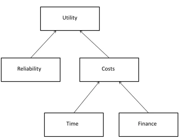
In order to construct complex multi-attribute utility functions it can be useful to consider utility hierarchies [20, 21]. We can represent such a hierarchy in graphical form. The overall utility is separated into the conditional utilities of its individual attributes, each of which is represented by a node. Arrows from each of the attributes into the overall utility node indicate that this is the ‘child’ node for each of the ‘parent’ attribute nodes. Each of the attributes can be separated into sub-attributes as necessary. The sub-attributes are the parent nodes of the child node for the corresponding attribute.

If, for each child node, the parent nodes are mutually utility independent, we call the resulting hierarchy a mutually utility independent hierarchy (MUIH) [8]. We can construct a utility function, given such a hierarchy, in the following way.

• For each parent set of sub-attributes at the lowest level of the hierarchy construct an additive or a multiplicative utility function for the child.

• Repeat this step for each node at the next level up in the hierarchy and continue this process until the overall utility is obtained.

In our case, if reliability is utility independent of costs and financial costs are utility independent of time costs then the utility functionU(R, Y, χ) can be written in terms of the following MUIH:

U(R, Y, χ) = q1UR(R) +q2UY,χ(Y, χ) +q3UR(R)UY,χ(Y, χ), (1)

UY,χ(Y, χ) = r1UY(Y) +r2Uχ(χ) +r3UY(Y)Uχ(χ), (2)

where 0< q1, q2, r1, r2<1,−qi≤q3 ≤1−qi,−ri≤r3 ≤1−ri fori= 1,2, and q1+q2+q3=

r1+r2+r3= 1. That is, we can represent the overall utility in terms of a binary utility function for

cost and reliability and the utility for cost in terms of a binary utility function for financial and time cost. We reduce the specification of a 3-attribute utility into the specification of three univariate utilities and trade-off parameters between them. This would facilitate elicitation. The MUIH is given in Figure 2. We discuss the specification of the trade-off parameters (q1, q2, q3, r1, r2, r3) in

a Section 4.1.3.

The following results provide insight into the relationship between the interaction parameter

q3and how a decision maker trades off between aggregate cost and reliability while keeping utility

constant. This is referred to as the marginal rate of substitution. The proofs for both results are given in the Supplementary Material.

Proposition 1. The marginal rate of substitution between aggregate cost and reliability has a monotonically decreasing relationship with the interaction parameter q3.

This result tells us that decreasing q3 will increase the value of reliability.

Proposition 2. Increasing the interaction parameterq3will decrease the utility level for aggregate

costs.

These propositions will be used to interpret the results from the simulation study in section 4.2.

The structure of a MUIH is not as restrictive as it may at first seem. We give the following result. The proof is given in the Supplementary Material.

Proposition 3. Suppose we have attributes a _{= (}a_{1, . . . ,}a_{n) such that} a_{i = (ai,1, . . . , ai,m}

i)

Figure 2: MUIH for the overall utility function for the allocation of reliability tasks.

To solve the decision problem, the expectations will be taken over the utility function for the reliability,UR(R).

Remark 1. If the utility function U(R) is a polynomial function of the reliability R, and the reliabilities for each fault type i,Ri(t), are analytically tractable, then, using the reliability growth model in Section 2, an analytic solution to the reliability task allocation problem will exist.

We can see this by considering the moments of the reliability. They are given by

EDEX|D

R(t)β ₌ I

Y

i=1



1− 1−Ri(t)β

λi J

Y

j=1

(1−pi,j)θj



.

Thus, for any integer β, we can evaluate all of the moments of R(t) analytically wheneverRi(t) can be analytically evaluated. Hence there will be an analytic solution using any of the usual parametric forms of the reliability such as Exponential or Weibull, as well as for non-parametric forms. In the illustrative example in Section 4 we consider Exponential failure distributions. We do so without loss of generality, as with non-constant failure rates we can always warp the time axis so that failure rates are constant over the warped axis.

3.2

Risk aversion and loss aversion

In general, preferences of decision makers have been shown to be risk averse [7], with some notable exceptions which we discuss below. We define risk aversion of a decision maker in the following way [21].

Definition 4. Risk aversion can be measured, for consequences of a lottery c, by g(c) =U′′(c), where U′′(·) is the second derivative of the utility function U. In this case g(c) < 0 for a risk averse individual,g(c) = 0 for a risk neutral individual andg(c)>0 for a risk seeking individual.

In general, individuals’ preferences are risk averse [19, 32] and this implies convex utility func-tions for costs and concave utility funcfunc-tions for benefits. That is, we defineU1,Y(Y), U1,χ(χ), U1,R(R)

such that∂2_U

1,Y(Y)/∂Y2<0,∀Y,∂2U1,χ(χ)/∂χ2<0,∀χ, and∂2U1,R(R)/∂R2<0,∀R.

do not satisfy such a solution: individuals generally discard components that are shared by all lotteries under consideration and individuals generally underweight outcomes that are probable in comparison to those obtained with certainty. They named these properties the isolation effect and the certainty effect respectively. The isolation effect relates to reference points. Any resulting wealth lower than the reference point is regarded as a loss and any resulting wealth higher than the reference point is regarded as a gain. This implies utility functions should be concave for gains and convex for losses from a reference point of anticipated wealth following the lottery.

The isolation effect implies that utility functions should represent loss averse rather than risk averse decision makers. Loss aversion is a property of prospect theory rather than utility theory. Consistency with the isolation effect in utility theory implies s-shaped utility functions around a reference point. There are many cases of such utility functions being used. It will be useful for our purposes to give a formal definition of loss aversion. Loss aversion is defined in the following way (page 238 of [34]).

Definition 5. Consider a utility function on consequence c, for whichc >0 is regarded as a gain andc <0 is regarded as a loss, of the form

U(c) =u(c), for c≥0, U(c) =µu(c), for c <0.

The utility function represents a loss averse individual if µ > 1 and a gain seeking individual if µ <1.

This suggests that a loss averse individual is focused on avoidance of losses with little attention on gains and a gain seeking individual is focused on seeking gains with little attention for losses [34].

Let us return to the idea of gains from lotteries. Suppose the references point as the anticipated consequence (e.g. wealth) following the lottery isw.

Remark 2. For a solution to satisfy preferences consistent with the isolation effect g(c)>0 for c < w andg(c)<0forc > w.

In terms of the reliability growth problem, the engineers would anticipate the product to be released and so a reasonable reference point for the reliability would beR0. Similarly, they might

anticipate to achieve their time on test target and so their reference point for time on test would be T0. In terms of cost, the budget for testing is Y0 and any spend under this could be thought

of as a gain. Therefore we take this as the reference point in the utility function. Other reference points are possible and utility functions could be adapted to these simply.

A utility function representing loss aversion U2,Y(Y) for cost would be defined such that ∂2_U

2,Y(Y)/∂Y2 > 0,∀Y, a utility function representing loss aversion U2,χ(χ) for time on test

would be defined such that

∂2_U 2,χ(χ) ∂χ2

(

>0, forχ < T0,

<0, forχ > T0,

and a utility function representing loss aversionU2,R(R) for reliability would be defined such that

∂2_U 2,R(R) ∂R2

(

>0, forR > R0,

<0, forR < R0.

We have given conditions for utility functions which represent risk aversion or loss aversion in decision makers. However, since we have defined a utility function over three attributes, we consider the multi-attribute preference behaviour implied by the resulting multi-attribute utility function. [29] extended the idea of risk aversion to multi-attribute utility functions.

Consider a twice differentiable utility function with positive derivatives in both variables, for two attributesa∈A, b∈B, on a closed interval from the real line wherea0< a1, b0 < b1. Then

(a1, b0) each with probability 0.5 to a lottery in which they receive (a0, b0) or (a1, b1) each with

probability 0.5.

The idea was extended to utility functions in more than two attributes. Suppose we have attributesa1, a2, . . . , an each defined on a closed interval on the real line. Then the twice

differen-tiable utility functionU(a) =U(a1, . . . , an) represents a multivariate risk averse (MRA) individual

if and only if each pair (ai, aj), i6=jrepresents a BRA individual for allak\{ai, aj}. The definition takes the same form for utility functions over multivariate risk neutral (MRN) and multivariate risk seeking (MRS) individuals.

We apply the definitions above to the general form of utility function we have developed for our problem. We obtain the following result, the proof of which is given in the Supplementary Material.

Proposition 4. A utility functionU(R, Y, χ)defined by the MUIH in (1) with twice differentiable increasingU(R)and decreasingU(Y), U(χ)represents preferences which are

1. MRA if and only ifr3>0,

2. MRN if and only ifq3= 0 andr3= 0, and

3. MRS if and only ifq3>0 andr3<0.

Thus, using the general form of the utility function, for both risk and loss averse conditional preferences, we can incorporate multivariate risk averse, neutral or seeking decision makers.

3.3

Discussion

We propose a multi-attribute utility function where gains and losses are evaluated on an attribute specific basis. Foundations for such a multi-attribute utility function were developed by [5] which is supported by several empirical studies concerning decision making under risk (e.g. [2, 4, 32, 25, 9]). We require a reference point for each attribute about which we assess loss or gain.

Reference points from prospect theory [19] are typically defined as status quo. However, our interests are reliability growth where the purpose is change not status quo. Measuring performance for this context in relation to targets is more sensible, such as in [10], and these should be aligned with the targets negotiated at the start of the project.

We seek to develop prescriptive decision support for project management in reliability devel-opment where well established protocols for eliciting expert subjective probabilities exist (see for example [3, 36, 15, 22]). We do not make use of probability weighting functions which represent distortions of probabilities and as such our approach is consistent with classical utility theory.

3.4

Suitable utility functions

For a risk averse preferences approach, we wish to define convex utility functions over financial costs of the reliability tasks and times on test and a concave utility function over reliability. Suitable utility functions which satisfy this for financial cost and time on test are therefore

U1,Y(Y) = 1−

Y Y0

2

U1,χ(χ) = 1−

χ χ0

2

.

We see that, in both cases, the utility of the best possible outcome (Y = 0, χ= 0) is 1 and the worst possible outcome (Y =Y0, χ=χ0) is 0. Also,g(Y) =−2/Y02<0 and so the utility function

represents risk aversion in cost. This is also true of the utility function for time on test. A concave utility function for reliability can be defined as

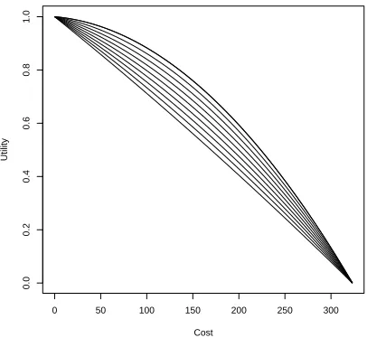
U1,R(R) =−γRAR2+ (γRA+ 1)R, (3)

so this utility function represents risk aversion. The parameterγRA represents the degree of risk aversion of the decision maker. We plot this utility function with different values ofγRA∈(0,1) in Figure 3. We see that the utility gives a reasonable range of possible risk aversion. Larger values ofγRA imply larger risk aversion.

0.0 0.2 0.4 0.6 0.8 1.0

0.0

0.2

0.4

0.6

0.8

1.0

Reliability

Utility

Figure 3: The risk averse utility function for expected reliability with different values ofγRA.

As the utility function for the reliability is a quadratic function in R, we have an analytic solution to the decision problem.

A suitable utility function representing loss aversion for reliability is

U2,R(R) =γLAR3+ (1−γLA)R2, (4)

whereγLA= 1/(1−3R0) to ensure the correct changepoint between convexity and concavity. We

see thatU2,R(0) = 0 andU2,R(R) = 1. Also,g(R) = 2−2(1−3R)/(1−3R0) and sog(R0) = 0,

g(R)>0 forR < R0 andg(R)<0 forR > R0 satisfying the condition in Remark 2. We give the

following proposition.

Proposition 5. ForULA(R) =γLAR3_{+ (1−γLA)R}2 _{to be monotonically increasing in R and}

possess the loss averse concavity requirement at R0 implies thatR0≥ 1₂ and as such−1₂ ≤γLA≤

−2or R0= 0 andγLA= 1.

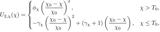
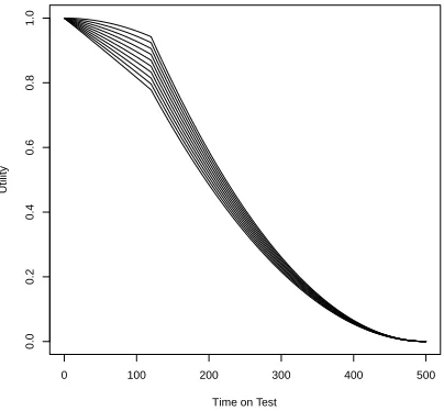
A suitable utility function for loss aversion of time on test is

U2,χ(χ) =



  

  

φχ

_χ

0−χ

χ0

2

, χ > T0,

−γχ

χ0−χ

χ0

2

+ (γχ+ 1)

χ0−χ

χ0

, χ≤T0,

whereφχ=−γχ+(γχ+1)/T andT = (χ0−T0)/χ0to ensure that the two functions are continuous

at the changepoint. We have one free parameterγχ. We see thatU2,χ(0) = 1 and U2,χ(χ0) = 0

representing the best and worst cases respectively. Also in the second caseg(χ) =−2γχ/χ2 0 <0

whenever χ > T0 for γχ > 0 and in the first case g(χ) = 2φχ/χ20 > 0 whenever χ < T0 for

γχ>0, φχ>0. This gives a utility function which satisfies Remark 2.

0 100 200 300 400 500

0.0

0.2

0.4

0.6

0.8

1.0

Time on Test

Utility

Figure 4: The loss averse utility function for time on test with different values ofγχ.

The utility function representing loss aversion for cost simply needs to be concave as any spend under budget is a gain. A suitable form is

U2,Y(Y) =−γY

Y0−Y

Y0

2

+ (γY + 1)

Y0−Y

Y0

,

where γY is a parameter which represents the degree of loss aversion of the decision maker. We see thatU2,Y(0) = 1 andU2,Y(Y0) = 0 representing the best and worst case scenarios respectively.

Also, g(χ) = −2γY/Y2

0 < 0 for γY > 0 and so the function is concave for all Y ∈ (0, Y0) and

satisfies Remark 2.

The utility function is plotted in Figure 5 for different values of γY ∈(0,1). We see there is a range of loss averse preferences possible using this utility function. Larger values ofγY lead to larger loss aversion.

Thus we see that all of the utility functions satisfy the preference behaviour observed in the isolation effect.

The certainty effect implies that preferences are typically not linear in probability: an increase in the probability of an event from 0 to 0.01 does not affect preferences in the same way as an increase from 0.3 to 0.31. For the analyses in this paper we simply remark that preference changes are observed to be fairly linear except in such extremes of probability.

In practice, the preferences of many engineers would not take the convenient forms identified in this section. For information on the elicitation of multi-attribute utility functions see pages 99-101 of [11].

3.5

Properties

Proposition 6. When confronted with a choice between two alternatives, each with the same mean value, a risk averse decision maker whose utility function is described by U1,R(Ri) =−γRARi2+

(γRA+ 1)Ri will have the same ranked preference for the options as a loss averse decision maker whose utility who is described by U2,R(Ri) = γLARi3+ (1−γLA)R2i if and only if the following condition is met (we denote the preferred option with subscript 1 and the other as 2).

E[R32]−E[R31]>

₁

γLA −1

0 50 100 150 200 250 300

0.0

0.2

0.4

0.6

0.8

1.0

Cost

Utility

Figure 5: The loss averse utility function for cost with different values ofγY.

The implications of Proposition 6 concern how such a loss averse decision maker will value skewness compared with symmetry. Simply, when choosing between two risks where the first two moments are equal, then the less skewed distributed is preferred.

Moreover, the alternative with the smaller variance is only preferred if accompanied by a sufficiently smaller third moment, and so its distribution is more symmetric.

Corollary 1. A loss averse decision maker whose utility function can be expressed asU2,R(Ri) = γLAR3

i+(1−γLA)R2i, whereRirepresents the reliability of the system andR0is the target reliability

of the programme, will prefer programme 1 over 2 under the following condition only.

E[R31]< E[R32]−3R0(Var[R2]−Var[R1]) if R0>

1 2.

Framing the utility in terms of reliability provides an interesting insight into the trade-offs being made during a reliability development programme between the individual item reliability and a fleet, as we can interpret E[Rk

i] as the expected proportion of a fleet ofk items surviving.

As such, the implication is that specifying high reliability targets on an item basis can result in products will poorer fleet reliability.

3.6

Comparison of utility functions

In this section we consider the utility functions representing risk and loss aversion of decision makers defined in the previous two sections. We compare them to two other sets of utility functions, based on an integer programming approach.

[33] used an integer programming approach to solve the decision problem, minimising the expected cost of the tasks subject to meeting the target reliability and being below the maximum testing time. Their approach was consistent in flavour, though not giving identical results, with the Bayesian solution using the following utility functions.

The approach was risk neutral with respect to financial cost and so

UY(Y) = 1− Y

Y0

In [33], two designs which met the target reliability were equally good and designs which did not were as poor as each other. Thus,

UR(R) =

(

0, ED{EX|D[R(t)]}< R0,

1, ED{EX|D[R(t)]} ≥R0.

Similarly, two designs which used less than the target test time were equally good and those which did not were equally poor. Thus,

Uχ(χ) =

(

0, χ > T0,

1, χ≤T0.

The linear programming approach assumes that two allocations which achieve the reliability target are equally good, though for two allocations equal in all else [33] would choose the one with higher expected reliability. We can build this preference for higher reliability even among designs which meet the target by using

UR(R) =

(

ED{EX|D[R(t)]}, ED{EX|D[R(t)]}< R0,

1, ED{EX|D[R(t)]} ≥R0.

Similarly, it would seem reasonable that of two designs which are equal in all other aspects and meet the target test time threshold, we would prefer the one with the shortest test time. Thus we could use

Uχ(χ) =







0, χ > T0,

1− χ

χ0

, χ≤T0.

We will call these two sets of utility functions the integer programming approach and extended approach respectively.

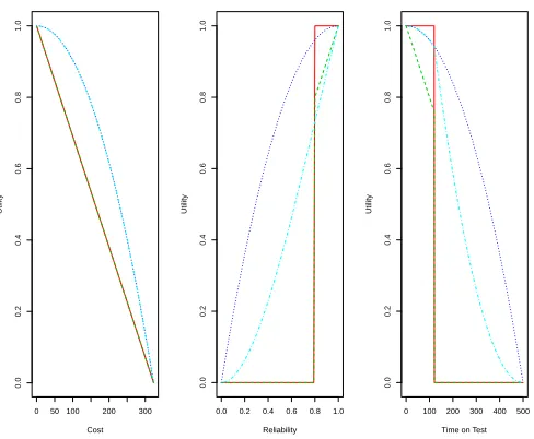
In Figure 6 we have plotted the utility functions for cost, reliability and time on test using each of the four approaches detailed above. The target reliability is set to R0 = 0.8, the target time

on test T0 = 120 and total budget Y0 = 500. The utility functions for the linear programming

approach are given in red, for the extended approach are given in green, for the risk averse approach in dark blue and the loss averse approach in light blue.

In the plot for cost we see that the utility functions for the integer programming approach and the extended approach are identical and linear. The utility functions for the risk averse approach and loss averse approach are also identical, givenγY = 1, and quadratic.

We see more differences in the utility functions for reliability. The integer programming ap-proach results in a simple step function with little sensitivity and the extended apap-proach represents a step function with a linear increase beyond the target reliability. There are differences between the risk averse and loss averse approaches in this case with the risk averse approach representing a decreasing gradient and the loss averse approach representing an increasing gradient below the target reliability.

Similarly, there are differences between all four utility functions for time on test. In particular, the utilities for the risk averse and loss averse approaches are very similar below the target time on test and very different above it.

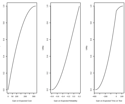
For the loss averse approach, the utilities are defined in terms of the gain on the reference points rather than purely on cost, reliability and time on test. These are plotted in Figure 7.

In each case zero on the x-axis represents the reference point (Y0, R0, T0 respectively). From

this we see the same pattern in each case, with risk seeking behaviour up to the target and then risk averse behaviour above the target value.

0 50 100 200 300

0.0

0.2

0.4

0.6

0.8

1.0

Cost

Utility

0.0 0.2 0.4 0.6 0.8 1.0

0.0

0.2

0.4

0.6

0.8

1.0

Reliability

Utility

0 100 200 300 400 500

0.0

0.2

0.4

0.6

0.8

1.0

Time on Test

Utility

Figure 6: Plots of the utility functions for cost, reliability and time on test using each of the four approaches.

4

Illustrative example and simulation study

4.1

Illustrative example

4.1.1 Background

During an elicitation exercise 15 design concerns and 14 reliability tasks are identified. This results in 16,384 possible combinations of tasks from which the programme manager must choose.

Each task has associated with it a cost of between 0 and 50 units and a duration of between 0 and 20 units. The target reliability is 0.8, the target time on test is 56 units, the maximum time on test is 84 units and the maximum total cost is 328 units.

In order to perform the analysis, the probabilities of each of the faults existing, λi, and the probabilities of finding the faults given that they do exist for each task,pi,j, need to be elicited. We also require the reliability functions for the faults. We assume exponential reliability functions of the form

Ri(t) = exp{−ψit},

where ψi is the rate of failures resulting from fault i. This can be elicited from an engineer by asking about the average number of failures of many similar items per unit time over a specified large period of time.

The final quantities which need to be elicited are the trade-off parameters for the binary utility functions and parameters for the conditional utility functions. We will investigate the sensitivity of the optimal allocation to the trade-off parameters in Section 4.1.3.

In this example, we simulate the λi from a uniform distribution between 0 and 0.5, approxi-mately 50% of thepi,j are equal to zero indicating that taskj will not find faulti and the rest are simulated from Unif[0,0.5] and each ψi is chosen to be 0.02. The trade-off parameters are chosen to beq1= 0.5, q2= 0.25, q3= 0.25 andr1= 0.5, r2= 0.5, r3= 0. That is, we are bivariate

0 50 100 200 300

0.0

0.2

0.4

0.6

0.8

1.0

Gain on Expected Cost

Utility

−0.8−0.6−0.4−0.2 0.0 0.2

0.0

0.2

0.4

0.6

0.8

1.0

Gain on Expected Reliability

Utility

−400 −200 0 100

0.0

0.2

0.4

0.6

0.8

1.0

Gain on Expected Time on Test

Utility

Figure 7: Plots of the utility functions against gain on expected cost, reliability and time on test using the loss averse approach.

4.1.2 Results

The expected utilities for the optimal design are 0.924, 0.758, 0.854 and 0.869 for the integer programming, extension, risk averse and loss averse approaches respectively. We see that the deterministic nature of the utility functions for the integer programming solution has resulted in a higher expected utility.

The optimal set of tasks for each approach is given in Table 1.

Table 1: The optimal set of tasks resulting from the four approaches.

Task 1 2 3 4 5 6 7 8 9 10 11 12 13 14

Integer × × X X _× X _× X _{× ×} X X _× X

Extended × × × X _× X _{× × × ×} X X X X

Risk Averse × × X X _× X _{× × × ×} X X X X

Loss Averse × × × X _× X _{× × × ×} X X X X

All four sets of utility functions offer similar optimal solutions, with the integer programming and risk averse approaches recommending performing 7 tasks and the extended and loss averse approaches 6. The integer programming approach offers an optimal allocation most different to the other three approaches. The extended and loss averse approaches give the same optimal set of tasks and only differ from the risk averse approach in whether to perform task 3.

We can also calculate the expected reliabilities, the costs and the times on test under each of the optimal solutions. The expected reliabilities are 0.837, 0.831, 0.865 and 0.831, the costs are 99.50, 118.98, 121.59 and 118.98 and the times on test are 33.48, 22.58, 31.43 and 22.58 for the integer programming, extended, risk averse and loss averse approaches respectively.

We see the integer programming approach has minimised cost subject to the other two con-straints whereas the extended and loss averse approaches have increased the cost slightly in order to reduce the time on test. The risk and loss averse approaches have found a solution which has higher expected reliability than the other approaches, while sacrificing cost compared to the loss averse and extended approaches and time on test to the integer programming approach.

0.0 0.2 0.4 0.6 0.8 1.0

0.0

0.2

0.4

0.6

0.8

1.0

Expected Reliability

Expected Utility

Figure 8: Expected reliability against expected utility for the integer programming (red), extended (green), risk averse (dark blue) and loss averse (light blue) approaches.

We see the differences between the integer programming (and extended) and risk and loss averse approaches. As expected reliability increases then expected utility decreases for the integer programming and extended approaches as we have not yet reached the target reliability and costs are increasing. In the risk and loss averse approaches increasing expected reliability can increase the expected utility if the increases in costs and time on test are small.

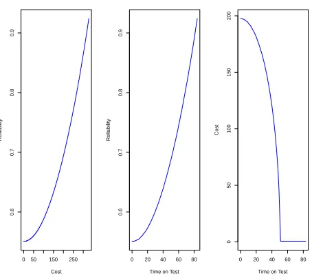
We can also consider the trade-offs between the different attributes in order to help engineers in their decision making. Trade-offs between the attributes can be represented using isoquants [6] in which we hold utility and one of the attributes constant and plot the curve of values for the other two attributes which lead to that utility value. These are given for the loss averse approach in Figure 9. Those for the risk averse approach show a similar pattern.

In all three cases the expected utility is held constant at 0.7. We see that as costs and time on test increase, then we need to increase reliability to maintain the same utility. Interestingly, the higher the cost or time on test, the more we have to increase reliability to maintain the utility value. In contrast, as time on test increases, costs need to be decreased at a faster rate to hold the utility constant.

4.1.3 Sensitivity to trade-off parameters

We investigate the sensitivity of the optimal solution for the loss averse approach to the specifi-cation of the trade-off parameters in the utility function. To do so we varyq1, q2, q3 and see how

this affects the expected utility of the optimal solution, tasks (3,4,5,6,7,8,10,13,14). We also investigate how large a change in the trade-off parameters it would take for this solution to no longer be optimal. This indicates the robustness of the solution to specification of the trade-off parameters.

Figure 10 gives plots of the expected utility of the optimal solution when we vary the values of

q1(left),q2(middle) andq3(right) and keep the other two parameters equal to each other. In each,

subsequent points which are the same symbol indicate that the optimal solution has remained the same whereas a change in the symbols of points indicates that the optimal solution has changed. We see from the plots that the optimal allocation of tasks is relatively sensitive to changes in

q1 andq2 in comparison to q3. If we consider the changes inq1 the optimal solutions at each of

0 50 150 250

0.6

0.7

0.8

0.9

Cost

Reliability

0 20 40 60 80

0.6

0.7

0.8

0.9

Time on Test

Reliability

0 20 40 60 80

0

50

100

150

200

Time on Test

Cost

Figure 9: Isoquants (left to right) for cost against reliability, time on test against reliability and time on test against cost for the loss averse utility approach.

0.0 0.2 0.4 0.6 0.8 1.0

0.88

0.90

0.92

0.94

0.96

0.98

1.00

q1

Expected utility

0.0 0.2 0.4 0.6 0.8 1.0

0.88

0.90

0.92

0.94

0.96

0.98

1.00

q2

Expected utility

0.0 0.2 0.4 0.6 0.8 1.0

0.88

0.90

0.92

0.94

0.96

0.98

1.00

q3

Expected utility

Figure 10: The expected utility of the optimal solution for varying values of trade-off parametersq1

(left),q2(middle) andq3(right). A change in symbol indicates a change in the optimal allocation

of tasks.

Table 2: The different optimal solutions asq1 is increased and the other trade-off parameters are

kept equal (q2=q3).

X X X X X X X X XX

Value ofq1

Task

1 2 3 4 5 6 7 8 9 10 11 12 13 14

0.00 × × × × × × × × × × × × × ×

0.05 × × × × × X _{× × × ×} X _{× ×} X

0.1,0.15,0.2 × × × × × X _{× × × ×} X X _× X

0.25,0.3 × × X X _× X _{× × × ×} X _{× ×} X

0.35,0.4,0.45 × × X X _× X _{× × × ×} X X _× X

0.5 × × × X _× X _{× × × ×} X X X X

0.55,0.6 × × X X _× X _{× × × ×} X X X X

0.65,0.7 X _× X X _× X _{× × × ×} X X X X

0.75 × × X X _× X _× X _{× ×} X X X X

0.8,0.85 × × X X X X _× X _{× ×} X X X X

0.9,0.95 X _× X X X X _× X _{× ×} X X X X

1 X X X X X X X X X X X X X X

4.2

Simulation study

In this section we compare the impact of decision makers who are loss averse and risk averse with respect to reliability. Firstly we consider an illustrative example to assess the potential implica-tions. Secondly we consider a simulation study to assess the propensity of such characteristics to result in disagreement.

4.2.1 Illustrative impact of loss versus risk aversion

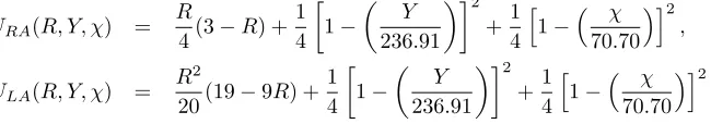
Consider a design under development where ten concerns (A-J) have been identified, each with an associated probability of being a fault. In addition, ten reliability tasks (1-10) have been identified and, for each concern, the probability each task will expose the concern assuming it is a fault has been elicited. All elicited probabilities have been provided in Table 3. Table 4 provides the associated cost and duration of each activity. The programme manager is charged with identifying the optimal set of tasks with a target reliability of 0.7, target cost of 236.91 and target duration of 70.70. In this example, we compare the difference in optimal programmes between managers who are loss averse (LA) on reliability (where γLA =−0.9 in (3)) and risk averse (RA) on reliability (where γRA = 0.5 in (4)). Both are assumed to be multivariate risk neutral and their multi-attribute utility functions are expressed as in the following.

URA(R, Y, χ) = R

4(3−R) + 1 4

1−

_Y

236.91

2

+1 4

h

1− χ

70.70

i2

,

ULA(R, Y, χ) = R

2

20(19−9R) + 1 4

1−

_Y

236.91

2

+1 4

h

1− χ

70.70

i2

.

The RA manager chooses a more expensive programme, performing tasks (2,3,4,9), that results in a higher expected reliability of 0.777, compared with the LA manager who performs tasks (3,4,9) which results in an expected reliability of 0.696, marginally below the 0.7 target. The additional activity chosen by the RA manager results in a 10% increase in project duration and a 50% increase in costs.

Table 3: Efficacy matrix showing the probability that each concern is a fault in the design and the probability that each task will reveal the concern assuming it is a fault.

Concern λi 1 2 3 4 5 6 7 8 9 10

A 0.087 0 0 0.52 0.09 0 0.55 0.46 0 0 0

B 0.360 0.72 0 0.49 0.78 0 0.06 0.76 0 0.5 0.86

C 0.473 0 0 0 0.65 0 0 0 0.09 0.13 0

D 0.465 0.68 0.45 0 0.67 0.91 0.09 0.32 0.54 0.74 0.68

E 0.035 0.13 0.68 0.72 0.21 0.61 0 0.26 0.84 0.63 0

F 0.246 0 0.38 0.99 0 0.35 0.44 0.11 0 0.04 0.31

G 0.126 0 0.3 0 0.56 0 0.19 0.98 018 0 0

H 0.011 0.61 0 0.44 0.4 0.95 0 0.48 0.9 0 0

I 0.037 0.87 0.28 0 0 0 0.18 0.51 0.37 0.89 0.54

J 0.449 0 0.89 0.55 0.01 0 0 0 0.98 0.53 0.01

Table 4: Task data on costs and duration.

Task 1 2 3 4 5 6 7 8 9 10

Cost 5.49 41.67 26.93 49.32 22.95 26.92 46.00 48.63 5.92 42.05 Duration 5.75 1.57 10.23 2.21 1.99 15.19 18.60 19.04 3.47 16.22

4.2.2 Simulation results

We have theoretical results on when the optimal allocations of tasks will coincide for risk averse and loss averse decision makers based on their conditional utilities for reliability. In this section we consider the effect of MRA, MRN and MRS preferences of the decision maker on the optimal allocation and the relationship between this and the choice of risk or loss averse preferences marginally.

We consider 3 different decision makers, one of whom is MRA, one who is MRN and one who is MRS. Using Proposition 4, suitable representative trade-off parameters are chosen for these individuals. In practice, these would be elicited from the decision maker. We consider the effect of risk averse versus loss averse preferences of each of these decision makers over the conditional utilities. We also consider the effect of the decision which is in the power of the engineering manager: that of how high to specify the target reliabilityR0 of the product. We vary the target

reliability between a low, medium and high level. All of the parameter values used in the simulation are given in Table 5.

Table 5: Parameter values used for the simulation into the effects of different multi-attribute risk preferences.

MRA q1= 1/3, q2= 1/3, q3= 1/3, r1= 1/3, r2= 1/3, r3= 1/3

MRN q1= 1/2, q2= 1/2, q3= 0, r1= 1/2, r2= 1/2, r3= 0

MRS q1= 1/3, q2= 1/3, q3= 1/3, r1= 2/3, r2= 2/3, r3=−1/3

R0 Low = 0.5, Medium = 0.7, High = 0.9

In each case we consider a reliability growth programme with 10 potential faults in the product and 10 reliability tasks which could be undertaken. We find the optimal allocation for each type of decision maker and reliability target in 100 simulations and calculate the proportion of optimal allocations each decision maker and reliability target combination has in common with each of the other combinations. This is then repeated 10 times in order to ensure the robustness of the simulation results.

−1 −0.8 −0.6 −0.4 −0.2 0 0.2 0.4 0.6 0.8 1 RA_MRA RA_MRN RA_MRS LA_MRA LA_MRN LA_MRS

RA_MRA RA_MRN RA_MRS LA_MRA LA_MRN LA_MRS

Low Target Reliability

−1 −0.8 −0.6 −0.4 −0.2 0 0.2 0.4 0.6 0.8 1 RA_MRA RA_MRN RA_MRS LA_MRA LA_MRN LA_MRS

RA_MRA RA_MRN RA_MRS LA_MRA LA_MRN LA_MRS

Medium Target Reliability

−1 −0.8 −0.6 −0.4 −0.2 0 0.2 0.4 0.6 0.8 1 RA_MRA RA_MRN RA_MRS LA_MRA LA_MRN LA_MRS

RA_MRA RA_MRN RA_MRS LA_MRA LA_MRN LA_MRS

High Target Reliability

The proportion of simulations which share the same optimal allocation for the different types of decision maker and reliability target. The sizes of the dots indicate the proportions, with larger dots indicating larger proportions.

We see that for MRA, MRN and MRS decision makers, whether they are risk averse or loss averse conditionally will have more of an effect on the final allocation of reliability growth tasks if the reliability target is lower. This is an important message, as it means for lower reliability products it will be necessary for engineers to be more careful about stating their preferences if they wish to obtain a suitable allocation of tasks. This has managerial implications, as for higher reliability products the reliability target can be set independently of the allocation of reliability tasks, whereas for lower reliability products the two decisions will need to be made in tandem. We also see a reasonable overlap in the optimal allocations of reliability tasks resulting from the MRA and MRN decision makers. Whether the decision maker is MRS or not (either MRA or MRN) does have a strong impact on the optimal allocation of reliability tasks.

The greater agreement between loss averse and risk averse decision makers for MRN whereq3

is 0 can be explained through Propositions 1 and 2. From Proposition 1, lowerq3results in greater

importance on reliability bringing the loss averse and risk averse decision makers closer together on how they rank programmes as trading between costs becomes less important. From Proposition 2, lower values of q3 make programmes more attractive, increasing utilities and decreasing their

differences.

It is important to check the robustness of the simulation results. In Table 6 we give the mean proportions of shared optimal allocations of reliability tasks for the combinations of type of decision maker and reliability target and their standard deviations over the multiple runs of the 100 simulations.

Table 6: Table showing the mean proportions of optimal task allocations that different combina-tions of decision maker and reliability target have in common over multiple simulation runs. Also given are the standard deviations in brackets.

Low Target Reliability

MRA RA MRN RA MRS RA MRA LA MRN LA MRS LA

MRA RA 1.00(0.00) 0.82(0.05) 0.42(0.06) 0.98(0.01) 0.84(0.05) 0.44(0.06) MRN RA 0.82(0.05) 1.00(0.00) 0.57(0.04) 0.80(0.05) 0.97(0.02) 0.58(0.04) MRS RA 0.42(0.06) 0.57(0.04) 1.00(0.00) 0.40(0.04) 0.55(0.03) 0.96(0.01) MRA LA 0.98(0.01) 0.80(0.05) 0.40(0.04) 1.00(0.00) 0.82(0.04) 0.42(0.05) MRN LA 0.84(0.05) 0.97(0.02) 0.55(0.03) 0.82(0.04) 1.00(0.00) 0.57(0.04) MRS LA 0.44(0.06) 0.58(0.04) 0.96(0.01) 0.42(0.05) 0.57(0.04) 1.00(0.00)

Medium Target Reliability

MRA RA MRN RA MRS RA MRA LA MRN LA MRS LA

MRA RA 1.00(0.00) 0.81(0.03) 0.43(0.04) 0.82(0.03) 0.92(0.02) 0.55(0.04) MRN RA 0.81(0.03) 1.00(0.00) 0.58(0.04) 0.66(0.04) 0.85(0.04) 0.71(0.04) MRS RA 0.43(0.04) 0.58(0.04) 1.00(0.00) 0.31(0.04) 0.46(0.04) 0.83(0.02) MRA LA 0.82(0.03) 0.66(0.04) 0.31(0.04) 1.00(0.00) 0.79(0.03) 0.40(0.04) MRN LA 0.92(0.02) 0.85(0.04) 0.46(0.04) 0.79(0.03) 1.00(0.00) 0.58(0.03) MRS LA 0.55(0.04) 0.71(0.04) 0.83(0.02) 0.40(0.04) 0.58(0.03) 1.00(0.00)

High Target Reliability

MRA RA MRN RA MRS RA MRA LA MRN LA MRS LA

MRA RA 1.00(0.00) 0.81(0.04) 0.41(0.08) 0.79(0.01) 0.92(0.03) 0.57(0.06) MRN RA 0.81(0.04) 1.00(0.00) 0.55(0.05) 0.64(0.04) 0.80(0.04) 0.73(0.04) MRS RA 0.41(0.08) 0.55(0.05) 1.00(0.00) 0.28(0.07) 0.39(0.06) 0.76(0.03) MRA LA 0.79(0.01) 0.64(0.04) 0.28(0.07) 1.00(0.00) 0.82(0.02) 0.41(0.06) MRN LA 0.92(0.03) 0.80(0.04) 0.39(0.06) 0.82(0.02) 1.00(0.00) 0.55(0.05) MRS LA 0.57(0.06) 0.73(0.04) 0.76(0.03) 0.41(0.06) 0.55(0.05) 1.00(0.00)

R0.

A summary of the simulation is provided in Table 7, where we see that switching between managers who are RA and LA with respect to reliability results in greater disagreement as we lower the target reliability. This is not surprising, as the higher a reliability target is, the less choice exists for programme managers.

Table 7: Proportion of simulations where a RA manager agreed with a LA manager, showing that agreement is higher for high reliability targets and MRN multiattribute preferences.

MRA MRN MRS

High reliability 0.98 0.97 0.97 Medium reliability 0.82 0.86 0.81 Low reliability 0.79 0.81 0.76

4.3

Implications

There are important implications resulting from the analyses in Section 4. In particular, we have seen that

1. The use of smooth utility functions to represent a decision maker’s preferences can give additional sensitivity around targets compared to constraint based methods. By considering risk averse and loss averse utilities we do not discount potentially attractive solutions close to targets.

2. In a multi-attribute utility approach, the optimal solution to the decision problem can be sensitive to the preference behaviour of the decision maker over multiple attributes simulta-neously. It is important for the analyst to elicit preferences over multiple attributes to come to a decision which is representative of the decision maker’s preferences.

3. The reliability target for high reliability products does not have an effect on whether there are different optimal allocations resulting from the different preference behaviours of the decision maker. From a managerial point of view, the reliability target can be set independently from the decision problem. For medium and low reliability products this is not the case.

5

Summary

We have investigated a Bayesian approach to the allocation of reliability tasks during product development. The optimal solution maximised the prior expectation of a utility function which represented the decision maker’s preferences over expected reliability, cost and time on test. To evaluate the expected reliability we utilised a reliability growth model which was developed with engineers in the aerospace industry. Suitable utility functions were identified using two approaches, a risk averse approach and a loss averse approach. The forms of these utility functions were consistent with observed preference of individuals in experiments.

The reliability growth model explicitly considers the process of reliability development un-dertaken by engineers. It is not seen as a black box approach and has advantages over other approaches in terms of buy-in. The Bayesian approach to the decision problem offers solutions which explicitly trade-off between the different attributes relevant to engineers and offers greater flexibility and sensitivity over integer programming, and other, approaches.

The utility functions developed display attractive properties but more work is needed in de-veloping flexible utility functions. The elicitation of utility functions in general, and trade-off parameters in utility hierarchies in particular, require more investigation in the literature.

In practice, not only the optimal allocation but also the optimal sequencing of tasks is important and, while the methods in this paper can reduce a large space of possible reliability tasks down to a much smaller space, it would be interesting to consider the use of the approach to the sequencing of reliability tasks.

References

[1] B. Aouni, C. Colapinto, and D. La Torre. Financial portfolio management through the goal programming model: Current state-of-the-art. European Journal of Operational Research, 234(2):536 – 545, 2014.

[2] I. Bateman, A. Munro, B. Rhodes, C. Starmer, and R. Sugden. A test of the theory of reference-dependent preferences. Quart.J. Econom, 62:479–505, 1997.

[3] T. Bedford, J. Quigley, and L. Walls. Expert elicitation for reliable system design. Statistical Science, 21:428–462, 2006.

[5] H. Bleichrodt, U. Schmidt, and H. Zank. Additive utility in prospect theory. Management Science, 55:863–873, 2009.

[6] A.C. Chiang. Fundamental Methods of Mathematical Economics. McGraw-Hill, 1984.

[7] J.C. Cox and G.W. Harrison. Risk Aversion in Experiments. Emerald Gorup, 2008.

[8] M. Farrow and M. Goldstein. Trade-off sensitive experimental design: a multicriterion, deci-sion theoretic, Bayes linear approach. Journal of Statistical Planning and Inference, 136:498– 526, 2006.

[9] G.W. Fischer, M. S. Kamlet, S. E. Fienberg, and D. Schkade. Risk preferences for gains and losses in multiple objective decision making. Management Science, 32:1065–1086, 1986.

[10] P. Fishburn. Mean-risk analysis with risk associated with below-target returns. American Economic Review, 67:116–126, 1977.

[11] S. French and D.R. Insua. Statistical Decision Theory. Arnold, 2000.

[12] H. Goel, J. Grievink, and M. Weijnen. Integrated optimal reliable design, production, and maintenance planning for multipurpose process plants. Comput. Chem. Eng, 27:1543–1555, 2003.

[13] S. Gurov, L. Utkin, and I. Shubinsky. Optimal reliability allocation of redundant units and repair facilities by arbitrary failure allocation or redundant units and repair facilities by arbitrary failure and repair distributions. Microelectron reliability, 35:1451–1460, 1995.

[14] W. Hallerbach, H. Ning, A. Soppe, and J. Spronk. A framework for managing a portfolio of socially responsible investments. European Journal of Operational Research, 153(2):517 – 529, 2004.

[15] R. Hodge, M. Evans, J. Quigley, and L. Walls. Eliciting engineering knowledge about reliabil-ity during design - lessons learnt from implementation.Quality and Engineering International, 17:169–179.

[16] C. Hsieh. Optimal task allocation and hardware redundancy policies in distributed computing systems. European Journal of Operational Research, 147:430–447, 2003.

[17] C. Hsieh and Y. Hsieh. Reliability and cost optimization in distribution computing systems.

Comp. Oper. Res., 30:1103–1119, 2003.

[18] A. Idrus, M.F. Nuruddin, and M.A. Rohman. Development of project cost contingency esti-mation model using risk analysis and fuzzy expert system.Expert Systems with Applications, 38(3):1501 – 1508, 2011.

[19] D. Kahneman and A. Tversky. Prospect theory: An analysis of decision under risk. Econo-metrica, 47:263–291, 1979.

[20] R. L. Keeney and H. Raiffa.Decisions with multiple objectives: preferences and value tradeoffs. Cambridge University Press, 1976.

[21] R. L. Keeney and H. Raiffa.Decisions with multiple objectives: preferences and value tradeoffs. Cambridge University Press, 1993.

[22] L. Walls L and J. Quigley. Building prior distributions to support Bayesian reliability growth modelling using expert judgement. Reliability Engineering and System Safety, 74:117–128, 2001.

[23] A. Nieto-Morote and F. Ruz-Vila. A fuzzy approach to construction project risk assessment.

[24] P.D.T. O’Connor. Practical Reliability Engineering. Wiley, 1991.

[25] J.W. Payne, D. J. Laughhunn, and R. Crum. Multiattribute risky choice behavior: The editing of complex prospects. Management Science, 30:1350–1361, 1984.

[26] D. Petrovic and O. Ak¨oz. A fuzzy goal programming approach to integrated loading and scheduling of a batch processing machine. Journal of the Operational Research Society, 59:1211–1219.

[27] D. Petrovi´c, R. Petrovi´c, and M. Vujo˘sevi´c. Fuzzy models for the newsboy problem. Inter-national Journal of Production Economics, 45(13):435 – 441, 1996.

[28] J. Quigley and L. Walls. Trading reliability targets within a supply chain using Shapley’s value. Reliability Engineering and System Safety, 92:1448–1457, 2006.

[29] S.F. Richard. Multivariate risk aversion, utility independence and separable utility functions.

Management Science, 22:12–21, 1975.

[30] A. Salo, J. Keisler, and A. Morton. Portfolio Decision Analysis : Improved Methods for Resource Allocation. Springer-Verlag, 2011.

[31] J.Q. Smith. Decision analysis: a Bayesian approach. Chapman and Hall, 1988.

[32] A. Tversky and D. Kahneman. Advances in prospect theory: cumulative representation of uncertainty. Journal of Risk and Uncertainty, 5:297–323, 1992.

[33] Johnston W, J. Quigley, and L. Walls. Optimal allocation of reliability tasks to mitigate faults during system development. IMA Journal of Management Mathematics, 17:159–169, 2006.

[34] P. P. Wakker. Prospect theory for risk and ambiguity. Cambridge Press, 2010.

[35] L. Walls and J. Quigley. Learning to improve reliability during system development.European Journal of Operational Research, 119(2):495 – 509, 1999.

[36] L. Walls, J. Quigley, and J. Marshall. Modeling to support reliability enhancement during product development with applications in the UK aerospace industry. IEEE Transactions on Engineering Management, 53:263–274, 2006.

Proof of Proposition 1

The utility function between reliability and costs is

U(R, C′) =q1U(R) +q2U(C

′

) +q3U(R)U(C

′

).

If we differentiate it with respect to reliability,

dU(R, C′

)

dR = (q1+q3U(C

′

))U′(R) + (q2+q3U(R))U

′

(C)dC

′

dR,

= 0.

The marginal rate of substitution is

MRS = dC

dR

= −U

′

(R)

U′

(C′

)

1−q2−q3(1−u(C

′

))

Differentating this with respect toq3,

dM RS dq3

= U

′

(R)

U′_(C′₎

(1−U(C′))

q2+q3U(R)

+(1−q2−q3(1−U(C

′

))U(R)) (q2+q3U(R))2

!

= U

′

(R)

U′

(C′

)(q2+q3U(R))2

((1−q2)U(R) +q2(1−U(C

′

)))

< 0

As the derivative of the marginal rate of substitution with respect toq3is constant, the relationship

is linear.

Proof of Proposition 2

To begin the proof,

U(C′(R)) = U0−q1U(R) 1−q1+q3(U(R)−1)

.

Differentiating this with respect toq3,

dC′(R)

dq3

= −U(R)−1

U′

(C′

)

U0−q1U(R)

(1−q1+q3(U(R)−1))2

< 0

As such, decreasing q3 increases the desirability of all programmes, improving the decision

maker’s choice.

Proof of Proposition 3

Proof. We use proof by contradiction. Suppose a decision problem has three attributes with utility functionUa, which can be further decomposed intoUa,1,Ua,2, and Ub. Further suppose that the

overall utility function is of the form of the MUIH

U = paUa+pbUb,

Ua = q1ua,1+q2Ua,2+q3Ua,1Ua,2,

for constantspa, pb, q1, q2, q36= 0. Then the utility function is given by

U =paq1Ua,1+paq2Ua,2+paq3Ua,1Ua,2+pbUb. (5)

If the attributes in the MUIH are utility independent then this utility function must take either the additive or multiplicative forms. The additive form implies that all sub-combinations of utilities are additive and so is not suitable in this case. Consider the multiplicative form. This implies that, for constantsca,1, ca,2 andcb,

1 +kU = (1 +kca,1Ua,1)(1 +kca,2Ua,2)(1 +kcbUb),

which can be expressed as

U = ca,1+ca,2Ua,2+kca,1ca,2Ua,1Ua,2+kca,1cbUa,1Ub

+kca,2cbUb+k2ca,1ca,2cbUa,1Ua,2Ub.

In order to be consistent with (5), we requireca,1=paq1,ca,2=paq2 andcb=pb. Further, each

of the cross terms involvingUb must have coefficient of zero. For example, we require

kca,1cb= 0⇒kpaq1pb= 0.

This implies thatk= 0. However this cannot be the case as we also require kca,1ca,26= 0. Thus

Proof of Proposition 4

Proof. All conditional utility functions are twice differentiable and assumed to be on [0,1] without loss of generality. We could defineV(Y) =−U(Y), V(χ) =−V(χ) to ensure positive first deriva-tives and change signs in the binary utility functions but this does not affect the proof. Consider the cost utilityU(C). Its cross derivative is

∂2_U(C)

∂Y ∂χ =q3U

′

(Y)U′(χ).

SinceU′(Y)>0, U′(χ)>0 for allY, χ >0, then using Theorem 1 in [29] this implies that we are BRS ifq3>0, BRN ifq3= 0 and BRA ifq3<0.

Let us now consider attributes R, Y. The cross derivative is

∂2_{U(R, C)}

∂R∂Y =r3U

′

(R)[q1U

′

(Y) +q3U

′

(Y)U(χ)].

We know thatU′(R)>0, U′(Y)<0, U(χ)>0, q1>0. We are therefore BRS forq3>0 ifr3<0,

ifq3= 0 we are BRA if eitherq3<−q1/U(χ), r3>0 orq3>−q1/U(χ), r3 <0 and we are BRN

forq3= 0 ifr3= 0.

If we consider the final pair of attributesR, χ, the relevant cross derivative is

∂2_{U(R, C)}

∂R∂χ =r3U

′

(R)[q2U

′

(χ) +q3U(Y)U

′

(χ)].

We see that we obtain BRS and BRN preferences under the conditions outlined previously. This completes the proof for MRN and MRS solutions.

BRA solutions result for q3 <−q2/U(Y), r3 <0 andq3 >−q2/U(Y), r3 >0. Combining the

conditions for MRA we have two candidates;r3<0, q3< mandr3>0,m < q¯ 3<0, where

m = min{−q1/U(χ),−q2/U(Y)},

¯

m = max{−q1/U(χ),−q2/U(Y)},

for allχ, Y. In the first case there is no solution as whenχ→χ0 andY →Y0thenm→ −∞. In

the second case asY →0 andχ→0 then U(Y)→1 andU(χ)→1 giving the result.

Proof of Proposition 5

Proof. We want to know the restrictions on γLA such that dULA(R)

dR ≥0 forR ∈[0,1]. We have ULA(R) =γLAR3_{+ (1−γLA)R}2_{and so}

dULA(R)

dR = 3γLAR

2_{+ 2 (1−γLA)R}

= R(3γLAR+ 2 (1−γLA))

For dULA(R)

dR ≥0 we require 3γLAR+ 2 (1−γLA)≥0 for R ∈[0,1]. Assume γLA <0 and then

2−γLA ≤3γLAR+ 2 (1−γLA)≤2 (1−γLA). We require 3γLAR+ 2 (1−γLA)≥0. Therefore

Proof of Proposition 6

Proof. Assuming two alternatives with the same first moment implies E[R1] = E[R2]. If alternative

1 is preferred to alternative 2 then the following is true for the risk averse decision maker,

E[−γRAR2

1+ (γRA+ 1)R1]>E[−γRAR22+ (γRA+ 1)R2],

which implies E[R2

1]<E[R22]. As the means are the same we have Var[R1]<Var[R2]. If alternative

1 is preferred to alternative 2 then the following is true for the loss averse decision maker,

E[γLAR31+ (1 +γLA)R21]>E[γLAR23+ (1 +γLA)R22].

This implies the following

γLA(E[R31]−E[R32])>(1−γLA)(Var[R2]−Var[R1]).

SettingγLA<0 gives the result.

Proof of Corollary 1

Proof. For the utility function to be loss averse about the target R0 we requireγLA = 1

1−3R0