Formalizing Emphasis in Information Visualization

City, University of London Institutional Repository

Citation

: Hall, K. W., Perin, C., Kusalik, P. G., Gutwin, C. and Carpendale, S. (2016).

Formalizing Emphasis in Information Visualization. Computer Graphics Forum, 35(3), pp.

717-737. doi: 10.1111/cgf.12936

This is the accepted version of the paper.

This version of the publication may differ from the final published

version.

Permanent repository link:

http://openaccess.city.ac.uk/16709/

Link to published version

: http://dx.doi.org/10.1111/cgf.12936

Copyright and reuse:

City Research Online aims to make research

outputs of City, University of London available to a wider audience.

Copyright and Moral Rights remain with the author(s) and/or copyright

holders. URLs from City Research Online may be freely distributed and

linked to.

City Research Online:

http://openaccess.city.ac.uk/

[email protected]

EuroVis 2016

R. Maciejewski, T. Ropinski, and A. Vilanova (Guest Editors)

( ),

STAR – State of The Art Report

Formalizing Emphasis in Information Visualization

K. Wm. Hall,1C. Perin,1P. G. Kusalik,1C. Gutwin,2and S. Carpendale1

1_{University of Calgary, Canada} 2_{University of Saskatoon, Canada}

Abstract

We provide a fresh look at the use and prevalence of emphasis effects in Infovis. Through a survey of existing emphasis frame-works, we extract a set-based approach that uses visual prominence to link visually and algorithmically diverse emphasis effects. Visual prominence provides a basis for describing, comparing and generating emphasis effects when combined with a set of general features of emphasis effects. Therefore, we use visual prominence and these general features to construct a new mathematical Framework for Information Visualization Emphasis, FIVE. The concepts we introduce to describe FIVE unite the emphasis literature and point to several new research directions for emphasis in information visualization.

1. Introduction & Motivation

Emphasis is an essential component of Infovis, and encompasses, for example:

• Highlighting regions of interest, e.g., coloring data points when brushing and linking to emphasize relationships;

• Animating data points using motion [BWC03,WB04] and flick-ering [WLMB∗14], which are efficient for catching a viewer’s attention; and

• Altering the size of data points to provide more detail or to increase their legibility relative to other data points, e.g., the many space-distortion techniques in the literature including overview+detail and zooming (see [CKB09] for a review). The commonality between these diverse techniques is that all of them make some data points more prominent than others. For example, when a visualization exploits highlighting to emphasize some data points, differences in the prominence of the data points arise from variations in color, or more specifically hue, a pow-erful visual variable. While emphasis effects in visualization can be created using any visual variable [CM84,Ber83,Mac86], Info-vis researchers have often focused on distortion and magnification techniques, e.g., [CM01,LA94,Kea98,PCS95,SA82]. These tech-niques create emphasis effects by manipulating magnification (i.e., by simultaneously manipulating the visual variables size and po-sition) where differences in the prominence of data points arise from variations in magnification. Recently, researchers have ex-plored new emphasis effects using, e.g., blur [KMH02,Hau06], transparency [Hau06], halos [OJS∗11], motion [BW02,HR07], and flicker [WLMB∗14]. This continued emergence of new emphasis effects has moved visualization research beyond existing empha-sis frameworks. Given the usefulness of previous frameworks, it is important to develop a new, more complete framework for

em-phasis in information visualization, i.e., a unifying description of emphasis that captures the breadth of the new and existing empha-sis effects. To address this challenge, we explore emphaempha-sis effects in five steps:

A review of existing emphasis frameworks

In this review, we introduce visual prominence as a means of dividing the data points within a visualization into subsets. This emerges from our analysis of previous frameworks. We use these emphasis subsets constructed on visual prominence to describe emphasis effects in visualizations and conceptually unify the di-verse emphasis effects in the literature.

A survey of classes of emphasis effects in visualization

In this discussion, we extract general features of emphasis ef-fects. For example, we elaborate on the often overlooked role of time in emphasis effects. We also introduce the concepts of: 1)

intrinsic emphasis effects– changes in the prominence of data points resulting from the initial visual mapping process when creating a visualization (e.g., coloring water and land differently on a map), and 2)extrinsic emphasis effects– changes in the prominence of data points resulting from applying visual effects on top of existing visualizations (e.g., applying a lens to a map).

An approach to generating emphasis effects

We show how visual prominence subsets and related general fea-tures of emphasis effects are a conceptual basis for generating emphasis effects for visualizations.

A formal framework: FIVE

We provide a Framework for Information Visualization Empha-sis (FIVE) that captures all previous emphaEmpha-sis frameworks, and expands on this work. FIVE is consistent with describing and generating emphasis effects using visual prominence subsets and our extracted general features of emphasis effects.

This is the authors' version of the work.

Opportunities for using FIVE

Using FIVE and its related concepts, we provide an initial ex-ploration of new opportunities and future directions in emphasis research. This outlook highlights many research challenges, and this STAR can support researchers as they undertake this work.

As we examine emphasis through each of the above steps, we focus on visual variables as a way to explore emphasis techniques because visual variables are integral to information visualization. In addition, we focus on the mechanics of emphasis using visual variables, rather than the details ofhowvisual variables create em-phasis for the viewer. Through focusing on the mechanics, we show how FIVE can use set-based mathematics to incorporate and ex-tend previous function-based frameworks, providing new ways to decide bothwhatto emphasize andhowto achieve this emphasis. In addition, FIVE offers a basis for studying the details of how em-phasis is connected to perception (see section7.4). For example, some techniques (e.g., visual links [GR15,SWS∗11]) point to how emphasis can arise not just from varying visual variables, but also by leveraging Gestalt concepts (e.g., connectedness in the case of visual links).

Frameworks that describe families of techniques have proven useful, e.g., [Fur86,LA94,CM01], in particular when they are de-scriptive, comparative, andgenerative [BL04,BL00]. Therefore, one of our goals when we set out to analyze the emphasis litera-ture was to create a unifying emphasis framework that would be descriptive, comparative, and generative. FIVE is a new mathemat-ical description of emphasis that exhibits these properties. FIVE incorporates several conceptual elements:

1. A set-based notation to describe visual prominence.

2. Timeas a key part of describing emphasis effects (e.g., time vari-ant and invarivari-ant methods).

3. The data duplication present in some emphasis effects. 4. The variable degree of continuity in emphasis effects. 5. The co-existence of intrinsic and extrinsic emphasis effects.

FIVE opens up new ways of thinking about emphasis while also being compatible with previous frameworks.

2. Reviewing Previous Frameworks

To understand emphasis effects, we first examine existing frame-works that describe emphasis effects in information visualization. We include three types of papers in this review:

1. Papers that define and review concepts related to emphasis as opposed to papers that introduce a single emphasis effect. Papers in this category are [CKB09,Fur86,Fur06,Hau06,Kea98,SA82]. 2. Papers that provide a taxonomy of emphasis related effects, i.e., [KMH02,PCS95]. Note that we include the taxonomy in [KMH02] for completeness, although it is brief.

3. Papers that provide mathematical frameworks that describe em-phasis effects. This category includes [CM01,LA94].

All these frameworks provide ways to systematically create em-phasis effects and describe relationships between various emem-phasis effects. There are other papers that provide significant overviews of emphasis techniques [LH10,LM10,Rob11,TGK∗14]; however, these have different contributions. Liang and Huang [LH10] take

a very focused look at one aspect of emphasis (i.e., highlighting), and provide a list of how objects have been highlighted in visualiza-tions. Lam and Munzner [LM10] discuss empirical considerations when deciding on the number of views and the relationships be-tween these views for a particular interface. Robinson [Rob11] con-siders a large range of visual variables as starting points for creat-ing highlightcreat-ing effects and proposes design criteria to qualitatively compare these highlighting effects. However, Robinson [Rob11] focuses on highlighting related elements across multiple views in the context of geovisualization, a particular emphasis use case. Fi-nally, Tominski et al. [TGK∗14] have a partially overlapping survey in that they look at existing lenses, which have often been used for emphasis. However, they focus on using the perspective of Magic Lenses [BSP∗94] to discuss different types of variations such as changes in representation. Therefore, though these additional pa-pers contribute to the emphasis literature, we confine our review of previous emphasis frameworks to [CM01,CKB09,Fur86,Fur06,

Hau06,Kea98,KMH02,LA94,PCS95,SA82].

2.1. Introducing A Set-Based Emphasis Language

Each of the previous frameworks covers a broad range of em-phasis effects. However, as a collection, the frameworks are dis-parate in their descriptions of emphasis. Therefore, to enable our survey of these frameworks, we first establish a simple set-based language. While the generative aspects of the previous frame-works all rely on functions, the discussions in the papers fre-quently use set-based terminology. Hauser uses the word “sub-set” over fifteen times [Hau06] to describe emphasis effects. Fur-nas uses the word seven and twenty-six times in his two pa-pers on fisheye views, [Fur86] and [Fur06]. In both of his pa-pers [Fur86,Fur06], Furnas focused on how to establish which sub-setof a dataset to represent through use of aDegree Of Interest

(DOI) function. Other previous frameworks also provide ways of emphasizing subsets of a dataset using function-based mathemat-ics e.g., [CM01,Kea98,LA94,Hau06]. This prevalence of set-based ideas was one of our first clues to investigate a set-based frame-work. In this paper, we embrace the already established vocabulary of sets to describe emphasis effects.

While there are many means by which one can emphasize some data points in a visualization, the visual commonality between var-ious emphasis effects is that some data points are made visually moreprominentthan other data points. For example, magnification, highlighting, and motion create emphasis on certain data points by making these data points more prominent than others (e.g., big-ger, brighter, and moving). In particular, the data points in a visu-alization that has emphasis form groups or sets of differing visual prominence.

We define the foreground set of data points,F, as the data points that are most prominent in a visualization. The background set,B, is the set of data points that are least prominent in a visualization. Depending on the nature of the visualization and emphasis effect, there can be data points of intermediate prominence betweenFand

F

M

B

Figure 1:F, M, and B characterize an overview+detail interface

for a map (fromwww.unfoldingmaps.org). Here, F, M and B partially overlap as some data points are visible in more than one view. The most prominent visualized data points are in F, the least prominent ones in B, and the ones with intermediate prominence are in M.

In Figure1, some data points visible inF are also visible inM, and some data points visible inM are also visible inB. The data points common to multiple subsets (e.g.,F andM) have multiple prominences. If there was no overlap between the three represented subsets of data (F,M and B), there would be no information in common between the three views. Therefore,F,MandBcan be, but need not be, mutually exclusive.

We use this set-based terminology of F, M, and B to ana-lyze visualizations from previous emphasis frameworks accord-ing to differences in data point prominence. The other factors we use for comparing previous frameworks are: 1) visual ables, and 2) the use of data suppression. Manipulating visual vari-ables [Ber83,CM84,Mac86] can be used to create emphasis effects. Data suppression, i.e., choosing to not show certain data points in a visualization, can also create emphasis effects since data points that are not represented have no visual prominence and are con-sequently less prominent than the represented data. Therefore, we analyze the previous framework papers using the perspective of sets (F,M, andB), visual variables and data suppression. We summa-rize our analysis of previous frameworks and highlight the cover-age of each framework in Figure2. Figure2shows that 1) previous frameworks mostly focus on the visual variablessizeandposition, and 2) only a few visual variables are discussed while some visual variables are never mentioned (e.g., motion and orientation). We group previous framework papers into three categories:

Magnification Papers that describe magnification emphasis

ef-fects, i.e., [CM01,LA94,Kea98,PCS95,SA82].

Beyond Magnification Papers that describe non-magnification

emphasis effects, i.e., [CKB09,KMH02,Hau06].

Data Suppression Papers that focus on the creation of emphasis

effects through data suppression, i.e., [Fur86,Fur06].

SPENCE AND APPERLEY [SA82] FURN

AS [F

ur86]

LEUNG AND APPERLEY [L

A94]

PL

AISAN

T E

T AL [PCS95]

KEAHEY [K

ea98]

CARPEND

ALE AND MON

TA

GNESE [CM01]

KOSARA E

T AL [KMH02]

FURN

AS [F

ur06]

HA

USER [Hau06]

COCKBURN E

T AL [CKB09]

FIVE

YEAR

POSITION * SIZE *

ORIENTATION * COLOR VALUE * COLOR SATURATION * COLOR HUE *

SHAPE * TEXTURE * MOTION **

FLICKER ** DEPTH ** ILLUMINATION ** TRANSPARENCY ** BLUR/CLEARNESS **

DATA POINTS DATA DIMENSIONS

Paper alludes to using visual variable in row

Paper does not discuss visual variable in row

1980 1990 2000 2010

Paper discusses visual variable in row

Figure 2:Analysis of existing emphasis framework papers

accord-ing to early and recent visual variables, chronologically ordered and grouped by similarities (using Bertifier [PDF14]) in terms of which visual variables the papers consider for creating emphasis effects. We demonstrate in this paper how FIVE can encompass any of these visual variables. Figure Legend: * early visual vari-ables [CM84,Ber83,Mac86]; ** recent visual variables [War12]. Note that we interpret what Spence and Apperley referred to as pulsed illumination [SA82] as flicker.

2.2. Magnification

The literature is full of work concerned with creating emphasis us-ing magnification and distortion techniques. Therefore, instead of detailing all the specific techniques, we focus on the frameworks that encompass these techniques. Magnification and distortion techniques (e.g., polyfocal projections [KS78], Spence and Apper-ley’s BiFocal Displays [SA82], Furnas’ work [Fur86], or the Elastic Presentation Framework [CM01]) have generally been created to provide people with views (usually magnified) that assist in some data-oriented task in a visualization. This has led to many mag-nification techniques, such as constrained lenses [CCF95,KR96,

with Magic Lenses [BSP∗94]), Melange [EHRF08] (which makes use of compressing regions), and JellyLens [PPCP12] (which fits the lens to data regions). All of these techniques create expanded focal regions by compressing other regions, generating distortion. This strategy has been applied to many datasets and visualiza-tions, such as trees [LRP95,MGT∗03], graphs [GKN05,TAvHS06], tabular visualizations [RC94], calendars [BCCR04], text docu-ments [RM93], flow visualizations [DHGK06], collaborative visu-alizations [VLS02], and lens-based approaches – see [TGK∗14] for a review of interactive lenses in visualization.

Magnification is the result of varying the visual variables size and position in an interrelated manner to create an emphasis effect.

F is the most magnified data subset,Bis the least magnified sub-set, andMis the set of subsets of varying magnification between the magnifications ofF andB. Magnification does not necessar-ily decrease monotonically as a function of increasing distances fromF as is exemplified by polyfocal displays (e.g., see Fig. 5a in [LA94]). Figure3shows a magnification-based emphasis effect in the style of the Elastic Presentation Framework (EPF) [CM01]. Despite their visual similarities, researchers can approach magni-fication techniques from a variety of algorithmic perspectives. We briefly summarize the perspective from each framework that fo-cuses on magnification: [LA94,PCS95,Kea98,CM01].

In 1994, Leung and Apperley [LA94] created a taxonomy for distortion-oriented presentation techniques. This taxonomy is for two-dimensional distorted images that are produced by applying a transformation function to an undistorted image. The transforma-tion functransforma-tions enlarge focal informatransforma-tion compared to contextual in-formation, but do not remove the context entirely (as would occur in a simple zoomed view). Instead, both the enlarged focal region and the reduced contextual region appear concurrently. The taxonomy is based on descriptions of the magnification functions for various distortion techniques.

Plaisant et al. [PCS95] provided presentational and operational taxonomies for browsing images. They focused on presenting an image at different magnifications, e.g., using an overview+detail display or zooming. This presentational taxonomy is divided into the static and dynamic aspects of presenting images. The dynamic aspects relate to ways of altering the magnification of the image, e.g., fixed zoom increments or continuous zooming. The static as-pects of the taxonomy relate to spatial and temporal relations be-tween the magnification levels provided to the viewer, e.g., the number of views and their coordination in an overview+detail in-terface. Fisheye views in this taxonomy are the result of using what Leung and Apperley [LA94] refer to as distortion-oriented tech-niques.

Keahey [Kea98] discussed the “generalized detail-in-context problem”. He applied nonlinear magnification fields [KR97] to two dimensional data representations and discussed how designers can use the resulting increased space dedicated to magnified regions.

In 2001, Carpendale and Montagnese [CM01] introduced the EPF as a means of applying magnification to two-dimensional data representations. The EPF considers placing the data representation on a pliable sheet that can be deformed in three-dimensional space with respect to the viewpoint. This approach encompassed all pre-vious magnification approaches and frameworks except those based

F

M

B

M

Figure 3:F, M, and B regions in a lens-based magnification

visu-alization of a map. The lens uses a Gaussian drop-off function in the style of the EPF [CM01]. The visualization uses a deformation of two visual variable (size and position) to make the data points in F more prominent than the ones in M and B. For this example, B is spatially between M regions, and corresponds to the inflection point in the Gaussian drop-off function. This example highlights how magnification need not decrease monotonically as a function of spatial distance from F. That is to say, there is not a strict spatial constraint on the relationship between F, M, and B.

on Spence and Apperley’s 1982 work [SA82] and some variations covered in Furnas’ 1986 paper [Fur86]. EPF focused on the inclu-sion of multiple focal regions of varying shapes, and the drop-off functions used to create the transition,M, between the focal re-gionsF, and the contextB. Carpendale and Montagnese also incor-porated lighting, shading, depth, and grid-based textures, to create more readable variations in magnification. Therefore, there are a variety of ways to create magnification emphasis effects, but all of them exhibitF,M,B.

2.3. Beyond Magnification

A few papers describe emphasis effects beyond magnification, i.e., emphasis effects using visual variables other than size and position (see Figure2).

Kosara et al.’s taxonomy [KMH02] focuses on ways to make the data points comprisingF more prominent compared to those ofMandBinstead of considering the relationships betweenF,M, andB. Their brief taxonomy divides emphasis techniques into three categories. Spatialmethods make use of magnification to create emphasis effects and fall into the previous section. Fordimensional

methods andcuemethods,Fcorresponds to what Kosara et al. call the “focus" region, andBis the “context." For a specific emphasis effect,Mmay or may not be empty. Figure4uses our set-based terminology to describe Kosara et al.’s blur function, which they introduce alongside their taxonomy.

F

M

B

Figure 4:Using our terminology to show how F, M, and B can

be used to describe the blur function discussed in [KMH02]. The underlying graph is a facsimile that we have created to emulate Kosara et al.’s function [KMH02]. Here, r∈[0,1]is the relevance value of a given data point. A data point is irrelevant if r=0and maximally relevant if r=1. The blur value b is a function of r, and b depends on the threshold t, the step height h, the maximum blur diameter bmax, and the gradient g. In terms of sets, F consists of the data points with a relevance r>t; the most prominent data points in the visualization. B consists of the data point(s) with r=

0, the least prominent data points. M consists of the data points with a prominence between the most prominent ones and the least prominent ones, with decreasing prominence as r decreases.

and rendering style. In this generalization of focus+context, Hauser suggests using a normalizedDOIfunction that takes on a value of 1 for the focus and 0 for the context, with intermediate values in between.Fcorresponds to the data points with aDOIvalue of 1.B

corresponds to displayed data points with the lowestDOIvalue – 0 if the entire dataset is shown.Mis all of the displayed data points with aDOIvalue between that ofBand 1. Hauser’s generalization only uses of a subset of the possible visual variables to makeF

more prominent compared toMandB. There are additional ways to alter prominence, e.g., other visual variables, as Figure2shows.

Cockburn et al. reviewed overview+detail, zooming, fo-cus+context, and cue-based techniques [CKB09]. The first three types of techniques are based predominantly on magnification. Cue-based techniques use differences in rendering styles (e.g., highlighting, blur, and visual proxies) instead of size to make some data points more prominent than others. This variation in render-ing style provides a means by which the prominence of some data points can be altered. The most prominent data points are part of

F, relative to other data points in the visualization, inMandB. To use blur as an example, when some data points are rendered crisply and others are blurry, the crisp data points are more readable than the blurry data points and the crisp data points formF. The most blurry data points formB, and depending on how the blur is varied across the visualization,Mcontains data points with intermediate blurriness, between that ofFandB.

December 1986

Dec 16 S M T W Th F S

Dec 22 Dec 29 Jan 6 Jan 12 16 -JACK SMITH 10pm Talk 11:30 Lunch -LEAVE MCC Pack Office Turn In: Badge, keys -MEET w/RAY ALLARD

3pm (His office) -BANKING

Close Austin Accounts -ALLERGY APT.

Get Shot & Pick up medicine (pay bill, too)

23 -CLEVELAND Thry 12/27 10:30 a.m. United flight 1037

29 5 6 12 13 30 -MOVERS Furniture Arrives Find out time... -START ARRANGING FURNITURE

--only 3 days to get settled

24 -CHRISTMAS EVE

Midnight Church Service

7 -MCC PTAC Starts 14 31 25 -CHRISTMAS Parents House 10AM -TOM’S BIRTHDAY

Get him a present After Lunch -DINNER W/DAVE

Coming over at 6:60 -NUTCRACKER BALLET 8:30pm 8 -MCC PTAC continues 15 1 -NEW YEARS (Hooray!!) -PARTY at Tom&Lynn’s 8pm... 26 9 -MCC PTAC continues 16 2 -BACK TO WORK -MARIS’S FIRST At Bellcore 17 3 11 18 4 17 -Leave Austin 6:30 a.m.

To North Carolina American Flgt 287

(4 days vacation) 18 -VACATION

North Carolina Coast 15

-CLEAN (Leaving) -BELLC

4 - 6 pm with -DINNER Debor Basil 10 t -FINISH (for p 22 -BROOK Dinner 6:30 -PACK for Cle 27 -RETURN Iv 1:1 United Arr 10 -MCC PT ends 28 -HOUD Aunt 7:30 Broe 20 -VACATION North Carolina Coast

21 -N.J. A 2:30 pm Sue at -FURNI put i 19 -VACATION North Carolina Coast

F

M

B

Figure 5:This image is a facsimile that we have created to emulate

Furnas’ [Fur86] fisheye view of a calendar. F consists of the most prominent data point – Monday, December 16. B consists of the least prominent data points, and M consists of the data points with prominence between that of F and B.

2.4. Data Suppression

In his seminal work on fisheye views [Fur86,Fur06], Furnas fo-cused on which data points to represent rather than how to rep-resent the chosen data points, and thus his work is more about data suppression. Furnas considers DOI functions as a way of deciding which data points a visualization should represent, i.e.

DOI functions enable judicious choices about what data points to suppress. Data suppression relates to filtering, one of the ear-liest and most common emphasis effects in information visualiza-tion [Shn94,WS92].

Furnas explored the notion of fisheye views from the perspective of cognitive psychology. He came to the conclusion that an indi-vidual’s recollections occur via the creation of emphasized subsets where individuals tend to recall items that are either of greata pri-oriimportance or of particular current relevance to them [Fur86]. Figure5shows Furnas’ example of a fisheye calendar [Fur86] de-scribed usingF,M, andB. Furnas defines the fisheye-DOI subset to be the set of points with aDOIgreater than some cut-off value given the current focal point. The most general form of the fisheye-DOI is Equation1(in [Fur82] as cited by [Fur06]).

DOIFE(x|.) =F(API(x),D(.,x)) (1)

Here, the DOI of a pointx (given the current focal point ‘.’) is a function of the a priori importance of x, API(x), and the distance between the focal point andx, D(.,x). Furnas explains distorted views, zoom viewing, and multiple window views, i.e., view+overview or view+closeup, in terms of the fisheye-DOI sub-set [Fur06]. In particular, Furnas contends that such techniques show the same information, i.e., the fisheye-DOI subset, but in dif-ferent manners. In this context, the fisheye-DOI subset is equivalent toFS

MS

DOI

1.0

0.0

Z-value

Context Focus Context

F

M

M

B

B

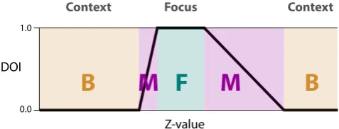
Figure 6:This image is a facsimile that we have created to

emu-late the one-dimensional trapezoidal DOI function of Doleisch et al. [DHGK06]. The z values represent some attribute of the data points. Assuming that the visualization shows all of the data points, the z value of a data point determines whether it is part of the focus (DOI=1) and therefore in F; part of the context (DOI=0) and in B; or somewhere in between (0<DOI<1) and therefore in M.

According to Hauser [Hau06], aDOIfunction is a function that returns a DOI value in[0,1]for each data point, i, in a dataset.

DOI(i) =1 ifiis part of the focus,DOI(i) =0 ifiis part of the con-text, and 0<DOI(i)<1 ifiis in between the focus and the context. As an example of this, Figure6shows the trapezoidalDOIfunction that Doleisch et al. describe [DHGK06].DOIfunctions have also been combined within a single view and using fuzzy logic to create

DOIfunctions describing features and sets of features [MKO∗08].

In Furnas’ work, theDOIfunction was not an end in itself. The

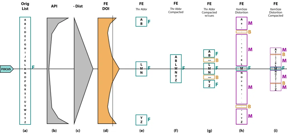
DOIfunction was meant to be used with some thresholdDOIvalue as a data filter to yield an appropriate fisheye-DOI subset [Fur06], i.e., a meaningful subset to be represented. Figure7is an annotated version of Furnas’ example of viewing a list using a DOI func-tion. This example makes it clear that deforming a representation is only one way to create an emphasis effect. Other ways to create emphasis effects include using visual cues and data suppression. The commonality between these possibilities is that they can all be described usingF,M, andB.

In Figure 7, an original ordered list of letters (a) is viewed through different fisheye views (e–i) according to aDOIfunction (d) that is the sum of an A Priori Importance (API) function (b) and a distance (Dist) function (c).

In Figure7(a), all the data points (elements of the list) are visible, and all data points have equal prominence as no data point is em-phasized. In this case, all data points belong toF, withM=B=/0. Figure7(e) is the subset of Figure7(a) that shows only the el-ements of the list that have a fisheye-DOI value greater than a threshold; this threshold is indicated by the thin vertical line in Figure 7(d). In this first subset, the fisheye list is created using data suppression, i.e., elements in the list whose fisheye-DOI is lower than the threshold are suppressed from the visualization. Be-cause all represented elements have the same prominence (in terms of font size), all visible elements belong to F. Since the visual-ization represents no elements with another level of prominence,

M=B=/0.

Figure 7(f) represents the same elements of the list as Fig-ure7(e), thus the same data suppression. However, in this case, the geometry is distorted, bringing all data points ofFtogether. Again,

M=B=/0.

Figure 7(g) re-introduces information about the fact that data points inF are spatially distant. In this case, the elements in B

are the letters between B and L and the letters between N and Y, which are represented using elision markers “...”. In (f), we still haveM=/0.

Figure7(h) differs from Figure7(e,f,g) in that all data points are visible, but their sizes are distorted according to theirDOIvalues.

Fconsists of the biggest letters (simply, the letter M in this case).

Bconsists of the smallest letters (letters D and V).Mconsists of all the remaining letters.

Figure7(i) consists of the sameF,MandBas in Figure7(h), but in Figure7(i) the data points are moved together. Note that most of the subsequent work based on Furnas’ fisheye views has focused on presentations similar to that of 7(i), which distort data points rather than simply suppressing data.

2.5. Previous Frameworks Summary

All of the reviewed emphasis frameworks have proven useful in information visualization research, with each being the inspiration for more than one subsequent emphasis technique. However, while some of the frameworks describe overlapping types of emphasis, none successfully describe all current emphasis variations. For ex-ample, while EPF [CM01] describes most magnification or dis-tortion approaches, it does not encompass Spence and Apperley’s original work [SA82]. Similarly, Hauser’s approach, based on Fur-nas’DOIfunction, includes a large part of the spatial and cue based approaches, but does not cover some of the possibilities in EPF. Despite the algorithmic and visual diversity of the emphasis effects found in previous frameworks, visual prominence and subsets (F,

MandB) are a common language for describing these effects as Figure7accentuates.

3. Describing Classes of Emphasis Effects

We now expand on our analysis of previous frameworks by describ-ingF,MandBfor classes of emphasis effects. To reasonably cover the extensive emphasis literature, we select pertinent examples to illustrate that visual prominence provides a conceptual bridge be-tween emphasis effects. For example, it is a common descriptive language for the visually distinct emphasis effects of zooming and highlighting.

FOCUS (b) API (c) - Dist (d) FE DOI A B C D E F G H I J K L M N O P Q R S T U V W X Y Z (a) Orig List F A B L M N Y Z (f) FE Thr Abbr Compacted F A B L M N Y Z (e) FE Thr Abbr F F F A B C D E F G H I J K L M N O P Q R S T U V W X Y Z (h) FE ItemSize Distortion F M M M M B B A B L M N Y Z (g) FE Thr Abbr Compacted w/cues F F F B B A B CDE F G H I J K L M N O P Q R

STU V W X Y Z (i) FE ItemSize Distortion Compacted F M M B M M B

Figure 7: This image is a facsimile that we have created to emulate Furnas’ selection vs. distortion discussion for a fisheye view of a

list [Fur06], annotated with F, M, and B. (a) is the original ordered list. (b) is an A Priori Importance (API) function over the list. (c) is a distance (Dist) function from the focus. (d) shows API+Dist, i.e. the sum of the A Priori Importance function and the Distance to focus function. (e,f,g,h,i) are possible Fisheye-DOI subsets representations that can be built based on the additive fisheye-DOI function in (d).

3.1. Time Invariant Emphasis Effects

An emphasis effect can be the result of using one or more visual variables to alter the visual prominence of data points. A time in-variant emphasis effect does not change with time. That is to say, it does not make use of such features as fade-in, fly-in, wipe and other forms of temporally based transitions. Examples of time invariant emphasis effects include: highlighting, blur, overview+detail and lens-based techniques, though one could incorporate temporal vari-ation into these effects.

Highlighting:Highlighting, or coloring, a data point in a

visu-alization emphasizes that data point. Coloring usually makes use of the visual variable hue and is often used in brushing and linking scenarios [BMMS91]. For example, in a scatterplot matrix visual-ization, brushing several points in a scatterplot will change their hue in that scatterplot and the linked scatterplots to emphasize the connection between brushed points [BC87].

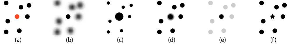
Figure8(a) illustrates highlighting one data point in a scatterplot. The red dot becomes the most visually prominent data point in the visualization. In Figure8(a), color is the strongest indicator of the visual prominence of the data points. Therefore,Fis the set of col-ored dots, andBis the set of black dots.Mis an empty set,M=/0, since the highlighting in Figure8(a) is binary.

Blurring: Photographers have created depth of field effects

based on blur for a long time. In photos involving depth of field effects, only part of the image is in focus while the rest of the image is out of focus and blurred. In the geographic visualiza-tion community, researchers have exploited blur to communicate uncertainty [Mac92]. Kosara et al. [KMH02] proposed a semantic version of depth of field as a means of emphasizing a subset of

a dataset. Figure8(b) illustrates this approach where one dot in a scatterplot is shown crisply while the others are blurred. Here, the crispness/blur is the major contributor to the differences in the vi-sual prominence of data points in agreement with the result of depth of field effects in photography.Fis the data point that is not blurred andBis the data points contained in the blurred portion of the vi-sualization. If there are varying degrees of blurriness, thenBwill be the most blurred data in the visualization,Mwill be the series of subsets of data that are increasingly less blurry, andFwill be the least blurry subset of data. Given that the blurring in Figure8(b) is binary, Figure8(b) only involvesFandB. Figure8(c–f) show ex-amples of emphasis effects that can be created in a similar fashion by manipulating other visual variables.

Overview+Detail:Overview+Detail is an emphasis effect where

the visual variables size and position are manipulated in order to create several views of a dataset such that different views have dif-ferent magnification values. Figure1shows the overview+detail technique for a map. The differences in the magnification values of the views causes data points in different views to have differing vi-sual prominence. In Figure1,Fis the set of data points in the view with the highest magnification.Bcorresponds to the data points in the view with the lowest magnification.Mconstitutes the data points in the view with intermediate magnification. In Figure1, the subsetsF,M, andBoverlap, i.e., they are not mutually exclusive. If there was no overlap between the three subsets, there would be no information in common between the three views.

Lens-based views: Similar to overview+detail, lens-based

exam-(a)

(b)

(c)

(d)

(e)

(f)

Figure 8:An emphasis effect created in a scatterplot by using (a) highlighting in red, (b) blurring, (c) size/area, (d) depth, (e) transparency

/ value, and (f) shape. In all cases, only one data point is emphasized, e.g., in (a) F is the only data point coloured red, B is the set of black data points, and M=/0.

ple of such focus-in-context lens-based views as applied to a map. As with overview+detail,F corresponds to the region of highest and uniform magnification, i.e., the focus.Bis the least magnified portion of the image. Finally,Mis the regions of the image with magnifications between that ofF andB. The regions comprising

F,M, andBneed not be continuous (e.g., see Figure3). For the visualization in Figure3,Mcan be further subdivided according to the differences in the magnification values, i.e., visual prominence, of data points within the drop-off region.

3.2. Time Variant Emphasis Effects

In contrast to time invariant emphasis effect, time variant emphasis effects involve time variations. For example, animations that em-phasize the appearance or disappearance of items are time vari-ant emphasis effects. For some emphasis effects, the data points that exhibit time varying behavior, e.g., flickering, are most visu-ally prominent, i.e.,F. For others effects, time is used to segregate views in which data points have differing visual prominence, e.g., zooming. Here we describe some classes of time variant emphasis effects.

Zooming:Zooming is an emphasis effect where views are

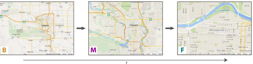
sepa-rated temporally instead of spatially [CKB09]. Because of the tporal separation, human memory plays a role in the creation of em-phasis effects based on zooming. For example, Figure9illustrates zooming in on the city of Calgary using Google Maps. In this ex-ample, an emphasis effect is created by varying magnification over time and perhaps by adjusting the labeling of the map. If one con-siders only the magnification component of the emphasis effect,B

is the data subset in the most zoomed out view;Fthe data subset in the most zoomed in view;Mis comprised of the intervening zoom states betweenFandB. Similar to overview+detail,F,M, andB

overlap, i.e., they are not mutually exclusive.

Assuming spatial zooming, the emphasis effect involves viewing subsets of the dataset with increasing magnification, i.e., varying the visual variables size and position with time. One could imagine an abrupt change fromBtoF without the use of any intervening views, i.e.,M= /0. Such a sudden change does not produce the smooth, gradually changing image that a viewer may expect while zooming. The degree to which a zoom appears to be discrete or continuous depends on the number of intervening views betweenF

andB, i.e., the number of prominence subgroups comprisingM.

Motion: Motion is a powerful emphasis effect where moving

objects are emphasized relative to stationary ones. Bartram et al. found that using motion to emphasize icons resulted in fewer un-detected icons compared to using color [BWC03]. Similarly, Ware and Bobrow [WB04] found that using motion to emphasize sub-graphs within a graph was more effective than a static highlighting method. Motion is an emphasis effect that varies the visual promi-nence of data points by varying the positions of data points with respect to time.

For example, consider an interactive node-link representation of a graph where selecting one node causes nearby nodes to oscillate while the other nodes remain stationary. The set of nodes that oscil-late are the most visually prominent nodes, i.e., they formF. The set of nodes that remain stationary are the least visually prominent nodes during the effect, i.e., they constituteB. Because of the bi-nary nature of motion in this example, there is no set of data points with intermediate visual prominence between that of the oscillating and stationary nodes, i.e.,Mis an empty set.

Flickering and Pulsing:Flickering is the cyclic variation of an

object’s transparency over time. Pulsing is the cyclic variation of an object’s size over time. Consider flickering or pulsing data points in a scatterplot. The most visually prominent data points, i.e.,F, are those that are flickering or pulsing. The data points that are not changing their appearance with time are less visually prominent, and consequently formB. Once again,Mis empty for both flick-ering and pulsing. Note that motion, flickflick-ering, and pulsing can simply be described in an unifying way: in all cases, the emphasis effect is created by changing the value of a visual variable (position, transparency, size) over time.

3.3. Emphasis Effect Descriptors

In the previous subsections, we described important classes of em-phasis effects in the common language of visual prominence, and broke down examples from these classes intoF,MandB. Through this process, three additional descriptors of emphasis effects be-came apparent: 1) time variant vs. time invariant, 2) degree of con-tinuity, and 3) multiple representations of data points. In this sub-section, we summarize these descriptors, and relate them toF,M

andB.

Time Variant vs. Time Invariant: Emphasis effects may or

F

M

B

t

Figure 9:Zooming in on Calgary, Canada using Google Maps. Map data: Google. The time arrow indicates that the viewer is zooming in

as time progresses. The views show how the viewer is transitioning from B to M and then from M to F. Even though the views are temporally dispersed, they all contribute to the emphasis effect that the viewer experiences.

Degree of Continuity:In terms of visual prominence, the

con-tinuity of the transition betweenF andB, as captured byM, can vary. For example,Mcan be empty for binary style emphasis ef-fects, e.g., traditional highlighting.Mmay correspond to a subset of data points that have a common visual prominence, from the per-spective of the emphasis effect, as in the overview+detail example shown in Figure1. Alternatively,Mcan contain multiple subsets of data points that differ in terms of their visual prominence (e.g., the lens drop-off region in Figure3), but are nevertheless bounded by the visual prominence of data points inFandB. More continuous transitions betweenFandBinvolve increasing numbers of visual prominence subsets comprisingM.

Multiple Representations of Data Points:F,MandBare not

necessarily mutually exclusive, though they are mutually exclusive for most emphasis effects. Zooming and overview+detail are exam-ples of emphasis effects where data points are represented multi-ple times in different views, and consequently have multimulti-ple visual prominences.

These emphasis effect descriptors and the setsF,M, andB pro-vide a basis for comparing emphasis effects. As an example of this, consider a three-level discrete zooming interface (e.g., Fig-ure 9), and a three-level static overview+detail view (e.g., Fig-ure1), both using the same representation of a map. By consid-ering three-level versions of each visualization, we are ensuring that the degree of continuity is the same for both, i.e., the num-ber of visual prominence subsets betweenF andBis the same for both. Both techniques also involve multiple representations of data points. However, they differ in that zooming is time variant while overview+detail is time invariant. For zooming, the multiple repre-sentations of a particular data point are spread out over time while they are spatially separated in overview+detail.

Zooming and overview+detail could use identical or different levels of magnification forF,M, andB. If the two techniques have differing magnification levels for any ofF,M, orB, then the relative changes in visual prominence can differ for the two techniques. If the techniques have the same magnification levels forF,M, andB, then one can consider whether or not the two techniques involve the same or differentF, M, and B subsets. Normally, zoom in-terfaces haveF, M, andB occupy the entire screen. In contrast, overview+detail interfaces generally divide the screen into

differ-ent regions that are allocated toF, M, and B. Because magnifi-cation is inherently tied to screen space, the views for each tech-nique cannot have the same magnification and show the same data while simultaneously occupying different amounts of screen space. Thus, the data points that compriseF,M, andBmust differ for the two techniques. Therefore, zooming and overview+detail are closely related, but zooming is not just a time separated version of overview+detail. This example shows howF,M, andBas well as temporal variation can be used to both describe and conceptually compare emphasis effects.

4. Intrinsic vs Extrinsic Emphasis Effects

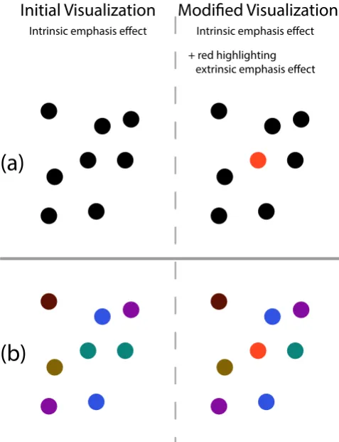
Previous frameworks have typically not considered the emphasis that is implicit in the original visual mapping chosen for a visu-alization. However, as we discuss in this section, differences in prominence due to the original visual mapping are not always neg-ligible, and can even interfere with emphasis effects. To take this into consideration, we introduce the concepts of: 1)intrinsic em-phasis effects– the baseline prominence differences between data points resulting from the initial visual mapping process when cre-ating a visualization, and 2)extrinsic emphasis effects– changes in the prominence of data points resulting from applying visual effects on top of existing visualizations. Figure10(a) illustrates the con-cepts of intrinsic and extrinsic emphasis effects as a data point in a scatter plot undergoes highlighting. The original visualization at the top left of Figure 10 has a position-based intrinsic emphasis effect while the visualization on the right now has a highlighting, i.e., an extrinsic emphasis effect. In this case, the initial intrinsic emphasis effect is both weak and distinct from the extrinsic emphasis effect.

4.1. Intrinsic Emphasis Effects

Mapping data dimensions to visual variables [Ber83, CM84,

For example, consider the intrinsic prominence differences be-tween visual features on a map. Cartographers generally represent longitude and latitude, or some projection thereof, using position. Water is represented as blue regions while land masses are colored to indicate countries or terrain. The cartographer (or a designer cre-ating a visualization) will rely on their considerable skills, their experience and the intent of the map when make these choices. The cartographer’s choices determine the intrinsic emphasis effect in the map.

4.2. Extrinsic Emphasis Effects

Extrinsic emphasis effects are additional visual variations applied on top of an existing visualization (which has its own intrinsic em-phasis effect) to create further variations in prominence.

Consider altering one or more visual variables of a given visual representation in order to create an extrinsic emphasis effect on top of the intrinsic emphasis effect. Assuming that the changes in visual prominence stemming from an extrinsic emphasis effect are sufficiently strong (e.g., color highlighting), one can consider that the intrinsic emphasis effect is negligible in comparison. In this case, one can focus solely on how the visual prominence of the data points is affected by the changes in the visual variables used to create the extrinsic emphasis effect.

For example, consider the map shown in Figure3. A lens-based distortion has been applied to an image, i.e., the distortion is an extrinsic emphasis effect applied on top of the existing intrinsic emphasis effect present in the map. If one focuses on magnification and not the details of the map, then the most visually prominent region in the image is the central flat region of the lens, and so this region isF.Bis the least magnified region.Mconsists of the regions of intermediate magnification.

In this example, the intrinsic and extrinsic emphasis effects are easily distinguished, i.e., we can easily seeF,BandMfor the lens while also still interpreting the map. Previous frameworks have as-sumed that the intrinsic emphasis effect is negligible compared to the extrinsic emphasis effect; however, this may not always be the case, as we discuss in the next subsection.

4.3. Conflicting Intrinsic and Extrinsic Emphasis Effects

We describe two examples where intrinsic and extrinsic empha-sis effects are in conflict and we discuss the implications of such conflicts. The first example uses a simple scatterplot visualization and shows how the intrinsic emphasis effect constrains the available choices for creating efficient extrinsic emphasis effects. The second example uses a more complex study [CDF14] and shows how con-sidering intrinsic and extrinsic emphasis effects can explain study results.

We start with a simple example illustrated in Figure10: high-lighting a point in a scatterplot. In Figure 10(a), data points are mapped toxandyto create the initial visualization. In Figure10(b), data points are mapped tox,yandcolorto create the initial visual-ization.

(b)

(a)

Initial Visualization

Intrinsic emphasis effect

Modified Visualization

Intrinsic emphasis effect + red highlighting

extrinsic emphasis effect

Figure 10:Potential conflicts between extrinsic and intrinsic

em-phasis effects. (a) shows a scatterplot where only the visual vari-able position is used to encode data point properties. In (b) hue is used in addition to position to encode additional information. The extrinsic emphasis effect that consists of highlighting the point in the center in red makes this point much more prominent in (a) while it fails at making this point much more prominent in (b). This is be-cause the intrinsic emphasis effect in (b), using the visual variable hue, conflicts with the extrinsic emphasis effect, which also makes use of hue.

The success of an extrinsic emphasis effect is dependent on the already existing intrinsic emphasis effect in a visualization. For the two initial visualizations in Figure10, consider highlighting a sin-gle point. In Figure10, the extrinsic emphasis effect consists of highlighting a data point by changing the data point’s color to red, using the visual variable hue. In Figure10(a), this extrinsic empha-sis effect is successful as it makes the emphasized data point much more prominent than other data points. In this case,F,M andB

As a more advanced example of competition between extrinsic and intrinsic emphasis effects, we explain the results of Chevalier et al.’s study [CDF14]. This study compares the effects of stag-gered and non-stagstag-gered animations on a tracking task during the re-arrangement of dots on a 2D plane. In the non-staggered condi-tion, dots move synchronously. In the staggered condicondi-tion, an in-cremental delay in start times across the moving elements is intro-duced. Figure11illustrates this experiment.

Trials for both conditions consist of three phases. In Phase 1, dots appear on a 2D plane, and some dots are highlighted, e.g., the red dot. In Phase 2, this highlighting disappears. In Phase 3, an animation (either staggered or non-staggered) takes place where the dots rearrange to a new configuration. Both types of animation use slow-in/slow-out effects for the motion of the dots, and all dots move the same distance. At the end of Phase 3, participants have to identify the originally highlighted dots.

The intrinsic emphasis effect in each trial arises from the initial positions of the points on the 2D plane (i.e., from the visual variable position). Phase 1 consists of applying an extrinsic emphasis effect using the visual variable hue on top of the intrinsic emphasis effect. For this extrinsic emphasis effect,F andBare the sets of colored and black dots, respectively. In Phase 2, this extrinsic emphasis ef-fect is removed, and participants must try to mentally maintain the original hue-basedFandB, which may conflict with the position-based intrinsic emphasis effect for the set of data points. The dots then begin to move to their new locations, with either a staggered or a non-staggered animation. Finally, at the end of the animation, the dots have new positions on the 2D plane, which result in a new intrinsic emphasis effect.

Given that the points in Chevalier et al.’s study are in a 2D Carte-sian environment, we can express the speed of the points, v, as

v=

r

dx dt

2

+

dy dt

2

. In the non-staggered condition, the dots have the same speed at each point in time, i.e.,vis constant across the points, andvvaries with time according to the chosen slow-in/slow-out effect. However, the dots are moving in different direc-tions, sodx_dt and dy_dt vary across the points. These differences in the

xandyspeeds create a new time-variant extrinsic emphasis effect based on motion. There is no guarantee that this extrinsic emphasis effect will align with the original position-based intrinsic emphasis effect or the previous hue-based extrinsic emphasis effect. There-fore, there are possibly several differentF subsets that the viewer sees during the experiment, and the viewer is supposed to be able to pick out the points that comprisedFfor the color-based extrin-sic emphasis effect. From the perspective of competing emphasis effects, the dot tracking task is nontrivial.

In the staggered condition, dots start moving at different points in time, sovis not the same for all of the dots at each point in time. This means that there is an even greater diversity in the movement of the dots during the staggered animations compared to the non-staggered animations. This greater diversity could lead to stronger motion-based emphasis effects, which would only be helpful in tracking and differentiating the original hue-basedF when these staggered animations make the originalF subset visually promi-nent relative to other data points in the visualization. The stronger emphasis effects of staggered animations would be detrimental if

they increased the visual prominence of other dots relative to those in the original hue-basedFas they would just increase the difficulty of the dot tracking task. This can explain Chevalier et al.’s observa-tions that staggering was only marginally beneficial in some cases and detrimental at times compared to their non-staggered anima-tion technique. The complexity of emphasis effects at play during the staggered animations is greater than during non-staggered an-imation, so there are more opportunities for viewers to encounter problems with tracking the dots.

A staggered animation for a set of dots moving between two con-figurations would result in particularF, Mand Bsubsets, i.e., a particular emphasis effect. This animation would only be benefi-cial for tracking the subset of the dots on a 2D plane that the an-imation makes visually prominent. Given that Chevalier et al. op-timized some of their staggered animations for the dots that were highlighted in Phase 1, we can expect that those particular stag-gered animations are only beneficial for tracking the dots for which the animations were optimized. This aligns with Chevalier et al.’s finding that their staggered animations only reduced task complex-ity for their arbitrarily chosen targets, i.e., dots highlighted in Phase 1 of a trial.

Visual prominence subsets (F,MandB) provide a new perspec-tive on Chevalier et al.’s experiment - that of competing intrinsic and extrinsic emphasis effects. Based on this, we have provided an explanation of the previously-unexplained results of Chevalier et al.’s study – that is, why staggered animation was not found partic-ularly useful for their tracking task. Given that position and speed are intimately related (the latter is the time derivative of the former), Chevalier et al.’s animation-based emphasis effects are intertwined with the position-based intrinsic emphasis effects amongst the dots. However, hue does not necessarily couple to either position or mo-tion. Therefore, it should come as no surprise that it is difficult to recall and follow theFof one extrinsic emphasis effect when there are other powerful emphasis effects at play that are coupled to each other. While the community has previously implicitly assumed that extrinsic and intrinsic emphasis effects are separable, this analysis shows how interactions between extrinsic and intrinsic emphasis effects are important. Our analysis of Chevalier et al.’s work also highlights that the concepts ofF,M,B, intrinsic emphasis effects, and extrinsic emphasis effects are tools that researchers can use to analyzing existing visualization literature.

5. Generating a Visualization with Emphasis

We have shown how the data points in a visualization can be di-vided according to visual prominence to create subsets (F,Mand

B) and that these subsets serve as a basis for describing and com-paring emphasis effects. We have also introduced a set of related concepts: time variant vs. time invariant emphasis effects, degree of continuity, multiple representations of data points, and intrinsic vs. extrinsic emphasis effects. In this section, we leverage these con-cepts to provide a three-step process for generating visualizations with extrinsic emphasis effects:

1. Determine an initial representation of the data. 2. Determine the contents of the setsF,MandB

Non-stagger

ed

Phase 1

highlighting

Phase 2

remove

highlighting

animation

Phase 3

Stagger

ed

Figure 11:An illustration with two dots of Chevalier et al.’s staggered vs. non-staggered animation experiment [CDF14]. The dashed lines

indicating the trajectories of the dots and the arrows indicating if a dot is moving in a particular frame were not visible in the experiment. Note that Phase 1 and 2 are the same for both animation types.

Step 1 yields a visualization with an intrinsic emphasis effect. Taken together, steps 2 and 3 create an extrinsic emphasis effect. For each step, we illustrate the advantages of using the concepts that we have introduced in the previous sections.

5.1. Determine an Initial Representation of the Data

By differentiating between intrinsic and extrinsic emphasis effects, it is clear that the initial representation of a dataset contains an em-phasis effect before any subsequent explicit emem-phasis effect, e.g., a lens-based effect, is applied. Determining an initial representa-tion for any dataset is a standard task in informarepresenta-tion visualizarepresenta-tion where a visualization designer maps data dimensions to visual vari-ables. An appropriate initial representation depends on the nature of the data, the tasks that are to be performed, and the charac-teristics of the people using the data. As an example of the com-plexity that an initial visualization can involve, consider visualiza-tions of streaming data. Visualizavisualiza-tions of streaming data can in-volve a variety of visual changes depending on: 1) how data points are mapped to visual variables, and 2) whether or not data points can appear/disappear in the visualization (see Cottam et al.’s tax-onomy [CLW12]). However, the choices made here, e.g., the visual variables used for the visual mapping process, will constrain subse-quent extrinsic emphasis effects and subsesubse-quent manipulations of the visualization.

5.2. Determine the Content ofF,MandB

As a visualization designer populatesF,MandB, the designer is choosingwhatthe extrinsic emphasis effect will emphasize. Using these sets as a basis for constructing extrinsic emphasis effects has the advantage that either set operations, functions (which are de-fined in terms of sets), or some combination thereof can be used to specify what should be emphasized in a visualization.

DOIfunctions are typically the basis of focus-and-context em-phasis effects. A designer could useDOIfunctions in conjunction with thresholds to populateF,MandBin our framework. There

is a long history of using functions to create magnification ef-fects [CM01,Kea98,LA94] (see Figure3). Furnas’ work withDOI

functions provides classic examples of using functions in conjunc-tion with thresholds to create subsets, specifically the fisheye-DOI subset [Fur86,Fur06] (see Figure7).

Alternatively, F, M, and B could be populated by applying set operations to pre-existing sets. These pre-existing sets could be intrinsic to the dataset as with set-typed data. Alsallakh et al. discuss set-type data in a recent survey of visualizations for sets [AMA∗14].

When defining F,M andB, a key consideration is the degree of continuity betweenF andB. If a designer wantsF to be very prominent relative to the other data points in the visualization, then they may opt to haveMempty, i.e., there is no intermediate promi-nence betweenFandB. This is the case for the emphasis effects in Figure8. Alternatively, a designer may want a more gradual transi-tion betweenFandB, in which case the cardinality ofMwill have to increase and the designer will have to define an increasing num-ber of subsets of data points to compriseM. A designer does not have to explicitly define the subsets ofM. For example, consider how the lens-based visualizations of the EPF [CM01] use func-tions to magnify data points (as illustrated in Figure3) and how Keahey’s work [Kea98] uses fields to magnify data points. These techniques specify the magnification of each data point, and im-plicitlyF,M, andBform based on magnification even though the techniques themselves do not explicitly create theF,M, andB sub-sets. Implicit definitions ofF,M, andBmay not provide the same level of control as explicit definitions.

A second important point is howF,MandBoverlap. If the de-signer wants to provide a person with multiple views on a dataset, then overlap in these views can be useful to, for example, show con-nections between the views. As such, the designer will have to rep-resent some data points multiple times in the visualization, and so

F,MandBwill overlap. The designer needs to decide which data points will be common betweenF,MandBeither explicitly (e.g., using a data point as reference point and making it common toF,M

5.3. Varying Prominence to differentiateF,MandB

As a designer chooses how to representationally varyF,M, andB, the designer is decidinghowthe viewer will experience the data points inFas being more visually prominent than those inMand

B. We highlight some of the new options for extrinsic emphasis effects, i.e., some alternative ways to make the data points inF

more prominent than thoseMandB. A designer will have to con-sider many context-dependent factors when creating an extrinsic emphasis effect for a visualization (e.g., what visual variables the visualization already uses and the nature of the intrinsic emphasis effect). Consequently, we do not attempt to cover all cases but in-stead provide some recommendations about varying prominence to differentiateF,MandB.

The increased visual prominence ofFrelative toBis related to the extent to which the representations ofFandBdiffer in terms of the visual variable the designer chooses for creating the extrinsic emphasis effect. For example, when using size, the difference in the visual prominence of the data points inFandBdepends on the magnitude of the size difference between the respective data points inFandB. Just-noticeable differences [SJ10] could be used to pro-vide indications about what are the minimum changes needed in a visual variable in order for a change in that visual variable to be no-ticeable to a viewer. Note that the visual encoding process in step 1 (creating an intrinsic emphasis effect) limits which visual variables remain available for differentiatingF,M, andB(when creating an extrinsic emphasis effect), as we discussed in Section4.3.

Some visual variables and combinations of visual variables re-main underexplored for creating emphasis effects (e.g., texture and orientation as shown in Figure 2) even though even though these visual variables strongly affect perception. Exploring the full set of visual variables and their time variation (e.g., varying either ori-entation or texture with time) may open up new and exciting em-phasis effects. If some visual variables are less overtly noticeable but still interpretable upon inspection, further work could develop “attention-based emphasis”. That is to say, emphasis effects that are unobtrusive unless someone is specifically considering a particular visual variable; this would leverage the principle that sensitivity to perceptual features is heightened with attention [Nei76,War12]. Also, when a visualization does not already use all visual variables, a designer can leverage the non-utilized visual variables to rein-force an extrinsic emphasis effect.

Lastly, different visual variables may be more or less effective at creating extrinsic emphasis effects depending on what other vi-sual variables are in use. For example, motion is a powerful means of creating emphasis effects; however, in visualizations where po-sition has meaning, large-scale motion effects could lead to erro-neous interpretations of the dataset. A designer needs to be aware of potential interactions between visual variables when creating ex-trinsic emphasis effects, and assessing such interactions should be part of the community’s research agenda.

6. FIVE: Framework for Information Visualization Emphasis

In the previous sections, we analyzed previous emphasis frame-works and a wide variety of emphasis effects. We showed how the visual prominence subsets F, M, andB are a basis for describ-ing, comparing and generating emphasis effects. In this section, we provide a mathematical framework that capturesF, M, and

B. Previous frameworks have provided mathematical formalisms (e.g., [CM01,Fur86,Hau06,LA94]). Mathematical formalism are powerful because they aid researchers and designers as they ana-lyze, describe, compare, generate and implement emphasis effects. Our analysis of emphasis effects has revealed five general features of emphasis effects, which we now summarize.

General Features of Emphasis Effects:

GF1 A wide variety of visualizations can be described in terms of subsets of data points of differing visual prominence (i.e.,F,M, andB).

GF2 There are time variant and time invariant emphasis effects.

GF3 Some emphasis effects represent data points multiple times, i.e., there can be overlap betweenF,MandB.

GF4 Emphasis effects have varying degrees of continuity between

F andB, i.e., varying numbers of intermediate levels of visual prominences comprisingM.

GF5 There are both intrinsic and extrinsic emphasis effects, which can interact with one another.

We now introduce an emphasis framework that captures these general features and the prominence subsetsF,MandB.

6.1. The FIVE Mathematics

Letpbe the prominence of the visual representation of a data point such that a high value ofpcoincides with a more prominent data point and a low value indicates a less prominent data point. Letpbe null for a data point that is not represented. An emphasis effect is the result of either representing a dataset such that data points have varyingp(e.g., highlighting dots in a scatterplot), or representing only a subset of a dataset (e.g., zooming in on a particular city in a map).

In order to formally demonstrate this, we first define the absence of emphasis. LetDbe the set of data points in a dataset. LetPd be

the set ofpvalues associated withd∈Dfor a given representation ofD.d∈Dcan have multiplepvalues because some techniques in-volve representing data points multiple times, e.g., overview+detail or zooming. By allowing data points to have multiplepvalues and representations, we are laying a foundation for supportingGF3.

A representation does not involve an emphasis effect when there are no differences in thePd sets associated with the data points in D, i.e.,∀a∈D∧ ∀b∈D:Pa=Pb. As soon as data properties are

mapped to visual variables, then∀a∈D∧ ∀b∈D:Pa=Pbis not

satisfied. A representation that satisfies∀a∈D∧ ∀b∈D:Pa=Pb