Generalising the Discriminative Restricted Boltzmann Machine

City, University of London Institutional Repository

Citation

:

Cherla, S., Tran, S.N., Weyde, T. & Garcez, A. (2016). Generalising the

Discriminative Restricted Boltzmann Machine.

This is the accepted version of the paper.

This version of the publication may differ from the final published

version.

Permanent repository link:

http://openaccess.city.ac.uk/14247/

Link to published version

:

Copyright and reuse:

City Research Online aims to make research

outputs of City, University of London available to a wider audience.

Copyright and Moral Rights remain with the author(s) and/or copyright

holders. URLs from City Research Online may be freely distributed and

linked to.

arXiv:1604.01806v1 [cs.LG] 6 Apr 2016

Boltzmann Machine

Srikanth Cherla, Son N. Tran, Tillman Weyde, and Artur d’Avila Garcez

School of Mathematics, Computer Science and Engineering City University London

Northampton Square, London EC1V 0HB. United Kingdom {srikanth.cherla.1,son.tran.1,t.e.weyde,a.garcez}@city.ac.uk

Abstract. We present a novel theoretical result that generalises the Dis-criminative Restricted Boltzmann Machine (DRBM). While originally the DRBM was defined assuming the{0,1}-Bernoulli distribution in each of its hidden units, this result makes it possible to derive cost functions for variants of the DRBM that utilise other distributions, including some that are often encountered in the literature. This is illustrated with the Binomial and{−1,+1}-Bernoulli distributions here. We evaluate these two DRBM variants and compare them with the original one on three benchmark datasets, namely the MNIST and USPS digit classification datasets, and the 20 Newsgroups document classification dataset. Results show that each of the three compared models outperforms the remain-ing two in one of the three datasets, thus indicatremain-ing that the proposed theoretical generalisation of the DRBM may be valuable in practice.

Keywords: restricted boltzmann machine, discriminative learning, hid-den layer activation function

1

Introduction

In the original work that introduced the DRBM its cost function was de-rived under the assumption that each of its hidden units models the {0,1} -Bernoulli distribution. We observe that while effort has gone into enhancing the performance of a few other connectionist models by changing the nature of their hidden units, this has not been attempted with the DRBM. So in this paper, we first describe a novel theoretical result that makes it possible to gen-eralise the model’s cost function. The result is then used to derive two new cost functions corresponding to DRBMs containing hidden units with the Binomial and {−1,+1}-Bernoulli distributions respectively. These two variants are eval-uated and compared with the original DRBM on the benchmark MNIST and USPS digit classification datasets, and the 20 Newsgroups document classifica-tion dataset. We find that each of the three compared models outperforms the remaining two in one of the three datasets, thus indicating that the proposed theoretical generalisation of the DRBM may be valuable in practice.

The next section describes the motivation for this paper and covers the re-lated work that led to the ideas presented here. This is followed by an introduc-tion to the Restricted Boltzmann Machine (RBM) in Secintroduc-tion 3 and its discrim-inative counterpart, the Discrimdiscrim-inative RBM (DRBM) in Section 4. The latter of these is the focus of this paper. Section 5 first presents the novel theoretical result that generalises this model, and then its two aforementioned variants that follow as a consequence. These are evaluated on three benchmark datasets, and the results discussed in Section 6. Section 7 presents a summary, together with potential extensions of this work.

2

Related Work

The subject of activation functions in has received attention from time to time in the literature. Previous work, in general, has either introduced a new type of activation function [18][20][6][14], carried out a comparative evaluation [4][7], or re-evaluated the significance of an existing activation function in a new context [2][3]. In the case of feedforward neural networks, while [4] concluded in favour of the Logistic Sigmoid activation function, recent work in [2] found a drawback in its use with deep feedforward networks and suggested the Hyperbolic Tangent function as a more suitable alternative to it. Even more recently, [3] highlighted the biological plausibility of the Rectified Linear activation function and its potential to outperform both the aforementioned activations without even the need to carry out unsupervised pre-training.

of sets of binary units all of which share the same values of weights. This idea was extended in [14] which introduced Rectified Linear activations for the hidden layer of the RBM. In the context of topic modelling, the replicated softmax RBM [6] was introduced which models the categorical distribution in its visible layer. All these variants of the RBM have been shown to be better suited for certain specific learning tasks.

It is often the case that a new type of activation function results in an im-provement in the performance of an existing model or in a new insight into the behaviour of the model itself. In the least, it offers researchers with the choice of a new modelling alternative. This is the motivation for the present work. As outlined above, effort has gone into enhancing the performance of a few mod-els in this way. We observe that it has not, however, been attempted with the DRBM. So here we address this by first introducing two new variants of the DRBM based on a novel theoretical result, and then comparing the performance of these and the original{0,1}-Bernoulli DRBM on benchmark datasets.

3

Restricted Boltzmann Machine

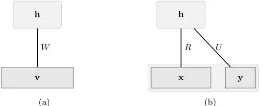
The Restricted Boltzmann Machine (RBM) [16] is an undirected bipartite graph-ical model. It contains a set of visible unitsv ∈Rnv _{and a set of hidden units}

h∈Rnh which make up its visible and hidden layers respectively. The two layers

are fully inter-connected but there exist no connections between any two hidden units, or any two visible units. Additionally, the units of each layer are connected to a bias unit whose value is always 1. The edge between theith_{visible unit and}

the jth _{hidden unit is associated with a weight w}

ij. All these weights are

to-gether represented as a weight matrixW ∈Rnv×nh_{. The weights of connections}

between visible units and the bias unit are contained in a visible bias vector

b∈Rnv_{. Likewise, for the hidden units there is a hidden bias vector c∈R}nh_.

The RBM is fully characterized by the parameters W, b and c. Its bipartite structure is illustrated in Figure 1.

h

v

W

(a)

h

x y

R U

(b)

Fig. 1: The architecture of an RBM (left) which models the joint distribution

The RBM is a special case of the Boltzmann Machine — an energy-based model [11] — which gives the joint probability of every possible pair of visible and hidden vectors via an energy function E, according to the equation

P(v,h) = 1

Ze

−E(v,h) ₍₁₎

where the “partition function”,Z, is given by summing over all possible pairs of visible and hidden vectors

Z =X

v,h

e−E(v,h)

. (2)

and ensures thatP(v,h) is a probability. The joint probability assigned by the model to the elements of a visible vectorv, is given by summing (marginalising) over all possible hidden vectors:

P(v) = 1

Z

X

h

e−E(v,h) (3)

In the case of the RBM, the energy functionE is given by

E(v,h) =−b⊤v−c⊤h−v⊤Wh. (4)

In its original form, the RBM models the Bernoulli distribution in its visible and hidden layers. The activation probabilities of the units in the hidden layer given the visible layer (and vice versa) are P(h = 1|v) = σ(c+W⊤_{v) and}

P(v=1|h) =σ(b+Wh) respectively, whereσ(x) is the logistic sigmoid function

σ(x) = (1 +e−x₎−1_{applied element-wise to the vectorx.}

Learning in energy-based models can be carriedgeneratively, by determining the weights and biases that minimize the overall energy of the system with respect to the training data. This amounts to maximizing the log-likelihood functionL over the training dataV (containingN examples), which is given by

L= 1

N

N

X

n=1

logP(vn) (5)

whereP(v) is the joint probability distribution given by

P(v) =e

−Ef ree(v)

Z , (6)

withZ =P

ve

−Ef ree(v)_{, and}

Ef ree(v) =−log

X

h

e−E(v,h). (7)

The probability that the RBM assigns to a vectorvn belonging to the training

the training data. Learning can be carried out using gradient-based optimisation, for which the gradient of the log-likelihood function with respect to the RBM’s parametersθneeds to be calculated first. This is given by

∂L

∂θ =−

*

∂Ef ree

∂θ

+

0 +

*

∂Ef ree

∂θ

+

∞

(8)

where h·i0 denotes the average with respect to the data distribution, andh·i∞

that with respect to the model distribution. The former is readily computed using the training dataV, but the latter involves the normalisation constantZ, which very often cannot be computed efficiently as it involves a sum over an exponential number of terms. To avoid the difficulty in computing the above gradient, an efficiently computable and widely adopted approximation of the gradient was proposed in the Contrastive Divergence method [19].

4

The Discriminative Restricted Boltzmann Machine

The generative RBM described above models the joint probability P(v) of the set of binary variablesv. For prediction, one is interested in a conditional distri-bution of the form P(y|x). It has been demonstrated in [9] how discriminative learning can be carried out in the RBM, thus making it feasible to use it as a standalone classifier. This is done by assuming one subset of its visible units to be inputsx, and the remaining a set of categorical unitsyrepresenting the class-conditional probabilitiesP(y|x). This is illustrated in Figure 1. The weight ma-trixW can be interpreted as two matrices R∈Rni×nh _{andU ∈R}nc×nh_{, where}

ni is the input dimensionality andnc is the number of classes andnv=ni+nc.

Likewise, the visible bias vectorb∈Rnv _{is also split into a set of two bias vectors}

— a vectora∈Rni _{and a second vectord∈R}nc_{, as shown in Figure 1.}

The posterior probability in thisDiscriminative RBM can be inferred as

P(y|x) = Pexp (−Ef ree(x,y))

y∗exp (−Ef ree(x,y∗))

(9)

where x is the input vector, and y is the one-hot encoding of the class-label. The denominator sums over all class-labels y∗ to make P(y|x) a probability distribution. In the original RBM,xandytogether make up the visible layerv. The model is learned discriminatively by maximizing the log-likelihood function based on the following expression of the conditional distribution:

P(y|x) = exp(dy)

Q

j(1 + exp(r⊤jx+uyj+cj))

P

y∗exp(dy∗)

Q

j(1 + exp(r⊤jx+uy∗j+cj))

The gradient of this function, for a single input-label pair (xi, yi) with respect

to its parametersθcan be computed analytically. It is given by

∂logP(yi|xi)

∂θ =

X

j

σ(oyj(xi))

∂oyj(xi)

∂θ

−X

j,y∗

σ(oy∗j(xi))p(y∗|xi)

∂oy∗j(xi)

∂θ

(11)

where oyj(x) =cj+r⊤jx+uyj. Note that in order to compute the conditional

distribution in (10) the model does not have to be learned discriminatively, and one can also use the above generatively learned RBM as it learns the joint distributionp(y,x) from whichp(y|x) can be inferred.

5

Generalising the DRBM

This section describes a novel generalisation of the cost function of the DRBM [9]. This facilitates the formulation of similar cost functions for variants of the model with other distributions in their hidden units that are commonly encoun-tered in the literature. This is illustrated here first with the {−1,+1}-Bernoulli distribution and then the Binomial distribution.

5.1 Generalising the Conditional Probability

We begin with the expression for the conditional distributionP(y|x), as derived in [9]. This is given by

P(y|x) =

P

hP(x,y,h)

P

y∗

P

hP(x,y∗,h)

=

P

hexp (−E(x,y,h))

P

y∗

P

hexp (−E(x,y∗,h))

(12)

whereyis the one-hot encoding of a class labely, and−logP

hexp(−E(x,y,h))

is the Free Energy Ef ree of the RBM. We consider the term containing the

summation overhin (12):

exp (Ef ree(x,y)) =−

X

h

exp (−E(x,y,h))

=−X

h exp   X i,j

xiwijyj+

X

j

uyjhj+

X

i

aixi+by+

X

j

cjhj





=−exp X

i

aixi+by

! X h exp   X j hj X i

xiwij+uyj+cj





Now consider only the second term of the product in (13). We simplify it by re-writingP

ixiwij+uyj+cj asαj. Thus, we have

X h exp   X j hj X i

xiwij+uyj+cj

 = X h exp   X j

hjαj

  =X h Y j

exp (hjαj)

=Y

j

X

k

exp (skαj)

(14)

wheresk is each of thekstates that can be assumed by each hidden unitjof the

model. The last step of (14) results from re-arranging the terms after expanding the summation and product overhandj in the previous step respectively. The summation P

hover all the possible hidden layer vectorshcan be replaced by

the summation P

k over the states of the units in the layer. The number and

values of these states depend on the nature of the distribution in question (for instance{0,1}in the original DRBM). The result in (14) can be applied to (13) and, in turn, to (12) to get the following general expression of the conditional probabilityP(y|x):

P(y|x) = exp (by)

Q

j

P

kexp (skαj)

P

y∗exp (by∗)

Q

j

P

kexp skα∗j

= exp (by)

Q

j

P

kexp (skPixiwij+uyj+cj)

P

y∗exp (by∗)

Q

j

P

kexp (skPixiwij+uy∗j+cj)

(15)

The result in (15) generalises the conditional probability of the DRBM first introduced in [9]. The term inside the summation over k can be viewed as a product betweenαj corresponding to each hidden unitjand each possible state

sk of this hidden unit. Knowing this makes it possible to extend the original

DRBM to be governed by other types of distributions in the hidden layer.

5.2 Extensions to other Hidden Layer Distributions

We first use the result in (15) to derive the expression for the conditional prob-ability P(y|x) in the original DRBM [9]. This will be followed by its exten-sion, first to the{−1,+1}-Bernoulli distribution (referred to here as the Bipolar DRBM)and then the Binomial distribution (the Binomial DRBM). Section 6 presents a comparison between the performance of the DRBM with these differ-ent activations.

sk ={0,1}. This reduces P(y|x) in (15) to

Pber(y|x) =

exp (by)Qj

P

sk∈{0,1}exp (skαj)

P

y∗exp (by∗)

Q

j

P

sk∈{0,1}exp skα

∗ j

= exp (by)

Q

j(1 + exp (αj))

P

y∗exp (by∗)

Q

j 1 + exp α∗j

(16)

which is identical to the result obtained in [9].

Bipolar DRBM: A straightforward adaptation to the DRBM involves replac-ing its hidden layer states by {−1,+1}as previously done in [1] in the case of the RBM. This is straightforward because in both cases the hidden states of the models are governed by the Bernoulli distribution, however, in the latter case each hidden unithj can either be a−1 or a +1, i.e. sk ={−1,+1}. Applying

this property to (15) results in the following expression forP(y|x):

Pbip(y|x) =

exp (by)Qj

P

sk∈{−1,+1}exp (skαj)

P

y∗exp (by∗)

Q

j

P

sk∈{−1,+1}exp skα

∗ j

= exp (by)

Q

j(exp (−αj) + exp (αj))

P

y∗exp (by∗)

Q

j exp −α∗j

+ exp α∗ j

.

(17)

Binomial DRBM: It was demonstrated in [18] how groups ofN (whereN is a positive integer greater than 1) stochastic units of the standard RBM can be combined in order to approximate discrete-valued functions in its visible layer and hidden layers to increase its representational power. This is done by repli-cating each unit of one layerN times and keeping the weights of all connections to each of these units from a given unit in the other layer identical. The key advantage for adopting this approach was that the learning algorithm remained unchanged. The number of these “replicas” of the same unit whose values are simultaneously 1 determines the effective integer value (in the range [0, N]) of the composite unit, thus allowing it to assume multiple values. The resulting model was referred to there as the Rate-Coded RBM (RBMrate).

The intuition behind this idea can be extended to the DRBM by allowing the states sk of each hidden unit to assume integer values in the range [0, N].

The summation in (15) would then beSN =PN_sk=0exp (skαj), which simplifies

as below

SN = N

X

sk=0

exp (skαj)

= 1 + exp (αj)

(N−1)

X

sk=0

exp (skαj)

= 1−exp ((N+ 1)αj) 1−exp (αj)

in (15) to give

Pbin(y|x) =

exp (by)Qj

PN

sk=0exp (skαj)

P

y∗exp (by∗)

Q

j

PN

sk=0exp skα

∗ j

= exp (by)

Q

j

1−exp((N+1)αj)

1−exp(αj)

P

y∗exp (by∗)

Q

j

1−exp((N+1)α∗

j)

1−exp₍α∗

j)

.

(19)

6

Experiments

We evaluated the Bipolar and the Binomial DRBMs on three benchmark ma-chine learning datasets. These are two handwritten digit racognition datasets — USPS [5] and MNIST [10], and one document classification dataset — 20 Newsgroups [8]. Before going over the results of experiments carried out on each of these, we describe the evaluation methodology employed which was common to all three and the evaluation metric.

Methodology A grid search was performed to determine the best set of model hyperparameters. The procedure involved first evaluating each of the trained models on a validation set and then selecting the best of these to be evaluated on the test set. When a dataset did not contain a pre-defined validation set, it was created using a subset of the training set. The initial learning rateηinit for

stochastic gradient descent was varied as {0.0001,0.001,0.01}. Early-stopping was used for regularisation. For this, the classification average loss of the model on the validation set was determined after every epoch. If the loss happened to be higher than the previous best one for ten consecutive epochs, the parameters were reverted back to their values in the previous best model, and training was resumed with a reduced learning rate. And if this happened five times, training was terminated. The learning rate reduction was according to a schedule where it is progressively scaled by the factors 1₂, 1₃, 1₄, and so on at each reduction step. The number of hidden units nhid was varied as {50,100,500,1000}. The

maximum number of training epochs was set to 2000, but it was found that training always ended well before this limit. The negative log-likelihood error criterion was used to optimise the model parameters. The DRBM generated a probability distribution over the different classes. The class-label corresponding to the greatest probability value was chosen as the predicted class. As all three datasets contain only a single data split, i.e. only one set of training, validation and test sets, the results reported here are each an average over those obtained with 10 model parameter initialisations using different randomisation seeds.

An additional hyperparameter to be examined in the case of the Binomial DRBM is the number of binsnbins. It corresponds to the number of states that

can be assumed by each hidden unit of the model. The value ofnbins was varied

Evaluation Measure In all of the prediction tasks, each model is expected to predict the one correct label corresponding to the image of a digit, or the category of a document. All the models in this task are evaluated using the average lossE(y,y∗), given by:

E(y,y∗) = 1

N

N

X

i=1

I(yi6=yi∗) (20)

whereyandy∗ are the predicted and the true labels respectively,N is the total number of test examples, andI is the 0−1 loss function.

6.1 MNIST Handwritten Digit Recognition

The MNIST dataset [10] consists of optical characters of handwritten digits. Each digit is a 28×28 pixel gray-scale image (or a vector x∈[0,1]784_{). Each} pixel of the image corresponds to a floating-point value lying in the range [0,1] after normalisation from an integer value in the range [0,255]. The dataset is divided into a single split of pre-determined training, validation and test folds containing 50,000 images, 10,000 images and 10,000 images respectively.

Table 1 lists the classification performance on this dataset of the three DRBM variants derived above using the result in (15). The first row of the table cor-responds to the DRBM introduced in [9]. We did not perform a grid search in the case of this one model and only used the reported hyperparameter setting in that paper to reproduce their result1_{. It was stated there that a difference} of 0.2% in the average loss is considered statistically significant on this dataset. Going by this threshold of difference, it can be said that the performance of all

Model Average Loss(%)

DRBM (nhid= 500,ηinit= 0.05) 1.78(±0.0012) Bipolar DRBM (nhid= 500,ηinit= 0.01) 1.84(±0.0007) Binomial DRBM (nhid= 500,ηinit= 0.01) 1.86(±0.0016)

Table 1: A comparison between the three different variants of the DRBM on the USPS dataset. The Binomial DRBM in this table is the one withnbins= 2.

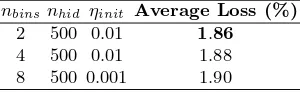
three models is equivalent on this dataset although the average accuracy of the DRBM is the highest, followed by that of the Bipolar and the Binomial DRBMs. All three variants perform best with 500 hidden units. It was observed that the number of bins nbins didn’t play as significant a role as first expected. There

seemed to be a slight deterioration in accuracy with an increase in the number of bins, but the difference cannot be considered significant given the threshold for this dataset. These results are listed in Table 2.

1 _{We obtained a marginally lower average loss of 1.78% in our evaluation of this model}

nbinsnhid ηinit Average Loss (%) 2 500 0.01 1.86 4 500 0.01 1.88 8 500 0.001 1.90

Table 2: Classification performance of the Binomial DRBM with different values of nbins on the MNIST dataset. While the performance does show a tendency

to worsen with the number of bins, the difference was found to be within the margin of significance for this dataset.

6.2 USPS Handwritten Digit Recognition

The USPS dataset [5] contains optical characters of handwritten digits. Each digit is a 16×16 pixel gray-scale image (or a vectorx ∈[0,1]256_{). Each pixel} of the image corresponds to a floating-point value lying in the range [0,1] after normalisation from an integer value in the range [0,255]. The dataset is divided into a single split of pre-determined training, validation and test folds containing 7,291 images, 1,458 images and 2,007 images respectively.

Table 3 lists the classification performance on this dataset of the three DRBM variants derived above using the result in (15). Here the Binomial DRBM (of

nbins = 8) was found to have the best classification accuracy, followed by the

Bipolar DRBM and then the DRBM. The number of hidden units used by each of these models varies inversely with respect to their average loss.

Model Average Loss (%)

DRBM (n= 50,ηinit= 0.01) 6.90(±0.0047) Bipolar DRBM (n= 500,ηinit= 0.01) 6.49(±0.0026) Binomial DRBM (8) (n= 1000,ηinit= 0.01)6.09(±0.0014)

Table 3: A comparison between the three different variants of the DRBM on the USPS dataset. The Binomial DRBM in this table is the one withnbins= 8.

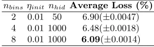
Table 4 shows the change in classification accuracy with a change in the number of bins. In contrast to the observation in the case of MNIST, here an increase innbins is accompanied by an improvement in accuracy.

6.3 20 Newsgroups Document Classification

nbinsηinit nhid Average Loss (%) 2 0.01 50 6.90(±0.0047) 4 0.01 1000 6.48(±0.0018) 8 0.01 1000 6.09(±0.0014)

Table 4: Classification average losses of the Binomial DRBM with different values ofnbins.

before the date. We used the 5,000 most frequent words for the binary input features to the models. This preprocessing follows the example of [9], as it was the second data used to evaluate the DRBM there. We made an effort to adhere as closely as possible to the evaluation methodology there to obtain results com-parable to theirs despite the unavailability of the exact validation set. Hence a validation set of the same number of samples was created2_.

Table 5 lists the classification performance on this dataset of the three DRBM variants derived above using the result in (15). Here the Bipolar DRBM outper-formed the remaining two variants, followed by the Binomial DRBM and the DRBM.

Model Average Loss (%)

DRBM (n= 50,ηinit= 0.01) 28.52(±0.0049) Bipolar DRBM (n= 50,ηinit= 0.001) 27.75(±0.0019) Binomial DRBM (n= 100,ηinit= 0.001) 28.17(±0.0028)

Table 5: A comparison between the three different variants of the DRBM on the 20 Newsgroups dataset. The Binomial DRBM in this table is the one with

nbins= 2.

Table 6 shows the change in classification accuracy with a change in the number of bins.

nbins ηinit nhiddenAverage Loss (%) 2 0.001 100 28.17(±0.0028) 4 0.001 50 28.24(±0.0032) 8 0.0001 50 28.76(±0.0040)

Table 6: Classification performance of the Binomial DRBM with different values ofnbins.

2 _{Our evaluation resulted in a model with a classification accuracy of 28.52% in}

7

Conclusions and Future Work

This paper introduced a novel theoretical result that makes it possible to gener-alise the hidden layer activations of the Discriminative RBM (DRBM). This re-sult was first used to reproduce the derivation of the cost function of the DRBM, and additionally to also derive those of two new variants of it, namely the Bipolar DRBM and the Binomial DRBM. The three models thus derived were evaluated on three benchmark machine learning datasets — MNIST, USPS and 20 News-groups. It was found that each of the three variants of the DRBM outperformed the rest on one of the three datasets, thus confirming that generalisations of the DRBM may be useful in practice.

It was found in the experiments in Section 6, that the DRBM achieved the best classification accuracy on the MNIST dataset, the Bipolar DRBM on the 20 Newsgroups dataset and the Binomial DRBM on the USPS dataset. While this does indicate the practical utility of the two new variants of the DRBM introduced here, the question of whether each of these is better suited for any particular types of dataset than the rest is to be investigated further.

Given the application of the result in (15) to obtain the Binomial DRBM, it is straightforward to extend it to what we refer to here as the Rectified Linear DRBM. This idea is inspired by [14], where the Rate-coded RBM [18] (analogous to the Binomial DRBM here) is extended to derive an RBM with Rectified Linear units by increasing the number of replicas of a single binary unit to infinity. Adopting the same intuition here in the case of the DRBM, this would mean that we allow the statessk to assume integer values in the range [0,∞) and thus

extend the summationSN in the case of the Binomial DRBM to an infinite sum

S∞ resulting in the following derivation:

S∞= ∞

X

sk=0

exp (skαj)

= 1 + exp (αj) ∞

X

sk=0

exp (skαj)

= 1

1−exp (αj)

(21)

with the equation for the Rectified Linear DRBM posterior probability in (15) becoming

Prelu(y|x) =

exp (by)Qj

P∞

sk=0exp (skαj)

P

y∗exp (by∗)

Q

j

P∞

sk=0exp skα

∗ j

= exp (by)

Q

j

1 1−exp(αj)

P

y∗exp (by∗)

Q

j

1 1−exp₍α∗

j)

.

(22)

References

1. Freund, Y., Haussler, D.: Unsupervised Learning of Distributions on Binary Vec-tors using Two Layer Networks. In: Advances in Neural Information Processing Systems. pp. 912–919 (1992)

2. Glorot, X., Bengio, Y.: Understanding the Difficulty of Training Deep Feedfor-ward Neural Networks. In: International Conference on Artificial Intelligence and Statistics. pp. 249–256 (2010)

3. Glorot, X., Bordes, A., Bengio, Y.: Deep Sparse Rectifier Neural Networks. In: In-ternational Conference on Artificial Intelligence and Statistics. pp. 315–323 (2011) 4. Gupta, B.D., Schnitger, G.: The Power of Approximation: A Comparison of Ac-tivation Functions. In: Advances in Neural Information Processing Systems. pp. 615–622 (1992)

5. Hastie, T., Tibshirani, R., Friedman, J., Franklin, J.: The Elements of Statistical Learning: Data Mining, Inference and Prediction, chap. 1

6. Hinton, G., Salakhutdinov, R.: Replicated Softmax: An Undirected Topic Model. In: Advances in Neural Information Processing Systems. pp. 1607–1614 (2009) 7. Karlik, B., Olgac, A.V.: Performance Analysis of Various Activation Functions

in Generalized MLP Architectures of Neural Networks. International Journal of Artificial Intelligence and Expert Systems 1(4), 111–122 (2011)

8. Lang, K.: Newsweeder: Learning to Filter Netnews. In: Proceedings of the 12th international conference on machine learning. pp. 331–339 (1995)

9. Larochelle, H., Bengio, Y.: Classification using discriminative restricted Boltzmann machines. In: International Conference on Machine Learning. pp. 536–543. ACM Press (2008)

10. LeCun, Y., Bottou, L., Bengio, Y., Haffner, P.: Gradient-based Learning Applied to Document Recognition. Proceedings of the IEEE 86(11), 2278–2324 (1998) 11. LeCun, Y., Chopra, S., Hadsell, R., Ranzato, M., Huang, F.: A Tutorial on

Energy-Based Learning. Predicting Structured Data (2006)

12. Lee, H., Grosse, R., Ranganath, R., Ng, A.: Convolutional Deep Belief Networks for Scalable Unsupervised Learning of Hierarchical Representations. In: International Conference on Machine Learning. pp. 609–616. ACM (2009)

13. Mohamed, A.R., Dahl, G., Hinton, G.: Acoustic Modeling using Deep Belief Net-works. IEEE Transactions on Audio, Speech, and Language Processing 20(1), 14–22 (2012)

14. Nair, V., Hinton, G.: Rectified Linear Units Improve Restricted Boltzmann Ma-chines. In: Proceedings of the 27th International Conference on Machine Learning (ICML-10). pp. 807–814 (2010)

15. Salakhutdinov, R., Mnih, A., Hinton, G.: Restricted Boltzmann Machines for Col-laborative Filtering. In: Proceedings of the 24th international conference on Ma-chine learning. pp. 791–798. ACM (2007)

16. Smolensky, P.: Parallel distributed processing: Explorations in the microstructure of cognition, vol. 1. chap. Information Processing in Dynamical Systems: Founda-tions of Harmony Theory, pp. 194–281. MIT Press (1986)

17. Sutskever, I., Hinton, G.: Learning Multilevel Distributed Representations for High-Dimensional Sequences. In: International Conference on Artificial Intelligence and Statistics. pp. 548–555 (2007)

19. Tieleman, T.: Training Restricted Boltzmann Machines using Approximations to the Likelihood Gradient. In: International Conference on Machine Learning. pp. 1064–1071. ACM (2008)