Influence of statistical uncertainty of component reliability estimations on offshore wind farm availability

Contents lists available at ScienceDirect

Reliability

Engineering

and

System

Safety

journal homepage: www.elsevier.com/locate/ress

Influence

of

statistical

uncertainty

of

component

reliability

estimations

on

offshore

wind

farm

availability

Matti

Niclas

Scheu

_,

_Athanasios

_Kolios

_,

_Tim

_Fischer

_,

_Feargal

_Brennan

b_{CranfieldUniversity,EnergyandPower,WhittleBuilding,BedfordshireMK430AL,UnitedKingdom}

a

r

t

i

c

l

e

i

n

f

o

Keywords:

Offshorewindenergy Operationsandmaintenance Maintenancemodelling Reliability

Statisticaluncertainty Availability

a

b

s

t

r

a

c

t

Offshorewindturbinereliability,oneoftheindustry’sbiggestsourcesofuncertainty,isthefocusofthepresent paper.Specificallytheimpactofuncertaincomponentfailuredistributionsatconstantfailurerateshasbeen investigatedwithrespecttoitsimplicationsforwindfarmavailability.Afullyprobabilisticoffshorewind simu-lationmodelhasbeenappliedtoquantifyresults;effectsshowninthispaperunderlinethesignificantimpactthat failureprobabilitydistributionshaveonassetperformanceevaluation.Itwasfoundthatwindfarmavailability numbersmayvaryintherangeupto20%justbychangingthedistributionsoffailuretoadifferentpattern;in particularthosescenariosinwhichextensivefailureaccumulationoccurredledtosignificantlossesin produc-tion.Resultsareinterpretedanddiscussedmainlyfromtheviewpointofanoffshorewindfarmdeveloper,owner andoperator,withimplicationsunderlinedforapplicationinstate-of-the-artoffshorewindO&M(Operationsand Maintenance)modelsandsimulationtools.

© 2017TheAuthors.PublishedbyElsevierLtd. ThisisanopenaccessarticleundertheCCBYlicense.(http://creativecommons.org/licenses/by/4.0/ )

1. Introduction

The offshore wind sector is today in a phase of rapid growth un- der multivariate market demands, such as an acceptable cost of energy level at a stable electricity supply and sustainable investment security for its shareholders. Electricity generated from offshore wind turbines will cover a share of up to 7.7% of Europe’s overall electricity consump- tion in 2030 by an installed power of 66 GW capacity [1] . The levelized cost of energy (LCoE) will thereby be driven down to an acceptable level; currently values of 80–100 €/MWh (megawatt hour) for offshore gener- ated electricity is aimed at for assets being located in European and US waters [2–6] . A long-term outlook from the UK government is even re- ferring to cost estimates of around 60 €/MWh by 2050; a value close to what onshore wind generation is achieving today – representing one of the most promising renewable energy technologies [7] .

Large investments are needed in order to achieve these ambitious targets. A figure of around €3billion per GW installed capacity is realis- tic for future investments according to Rubel et al. [8] . The same report addresses the desire for a commensurate risk-return balance from an investor’s perspective in order to attract investments in the field. The European Union presents a scenario in which fewer investments may be made in offshore wind due to a ‘struggle of de-risking ’ the industry [2] .

∗_{Correspondingauthorat:Ramboll,attn.MattiScheu,Stadtdeich7,20095Hamburg,Germany.}

E-mailaddress:[email protected](M.N.Scheu).

Various different risk sources are thereby relevant for the offshore wind industry. A number of publically available reports address those, such as [9] where the focus is on a methodology for financial assess- ment of a project; [10] which presents a comprehensive risk assessment framework aimed at new technologies with a strong technical focus; and [11] in which internal and external risk sources, specifically for large-scale offshore wind application, are assessed. All reports refer to, amongst other factors, risks associated with asset reliability. Other im- portant factors, such as ecological risks, political risks, risks in the supply chain, risks related to project financing or risks related to health, safety and the environment are omitted at this point due to the present work having a different focus.

Asset reliability is defined as the ‘ability of an item to perform a re- quired function under given conditions for a given time interval ’[12] . The reliability of the item, i.e. the asset ‘offshore wind farm ’, depends on, amongst others, the reliability of single wind turbines – respectively their systems, subsystems and components, as well as cabling, grid con- nectors and on– and offshore substations. A common term used to ex- press the reliability of an item is the so-called failure rate (FR), describ- ing the number of failures per unit of time [12] . As described thoroughly in [13,14] , the FR is, for many applications, not constant over time. This characteristic has also been observed for onshore wind energy convert- ers (WECs) which are, from a technology perspective, to some extent

http://dx.doi.org/10.1016/j.ress.2017.05.021

Availableonline5May2017

comparable with their offshore counterparts [15] . Time dependence of failures is related to the technical properties of the system or component. Examples of time and loading dependent failures are, for example, the wear out of gear teeth; in contrast the shutdown of a control system often unexpectedly occurs at random time intervals. The latter is a pat- tern which can specifically be observed for new, unproven concepts for which failure modes and mechanisms are not fully understood [16] .

Although it is understood that FRs are not constant throughout the lifetime of offshore WECs, most studies providing publically available reliability figures rely on this simplification [15–19] . All studies men- tioned, however, refer to the given fact that there are variations in com- ponent and system FRs over time, mostly qualitatively estimating a life- time failure distribution of an offshore WEC in the shape of a bathtub curve. Carroll et al. ’s most recent publication [19] , attempts, amongst other factors, to understand the statistical distributions of offshore WEC failure intensities over time. Their studies are based on the operational data of 350 turbines, where two thirds are in operation for three to five years and around one third for more than five years. From the presented data, there is no clear failure pattern observable which would allow for verification of scenarios suggested in former studies. In other words, this means that the statistical distribution of wind turbine reliability over the assets ’ lifecycle is yet to be understood.

Studies, such as the comprehensive report of Feng et al. [20] , illus- trate the significant impact that reliability figures have on offshore wind farm availability – a predominant measure of indicating the level of per- formance of offshore wind operations; availability here is defined as the ‘ability to be in a state to perform as and when required, under given conditions, assuming that the necessary external resources are provided ’ [12] . Positive financial turnovers may only be made in periods of avail- ability, i.e. when the WECs are in operation, thus producing electricity to be fed into a grid.

As many component failures potentially lead to stoppage of the WECs, the relationship between reliability and availability is obvious. This is addressed in several works introducing technical concepts that aim to improve reliability or allowing for early fault detection, minimis- ing the impact of a developing fault. Odgaard [21] , presents different fault tolerant control concepts as a way to maximise reliability. Other studies focus on early fault detection for instance by condition moni- toring systems [22] , or use of SCADA (Supervisory Control and Data Acquisition) information [23] .

It should, however, be noted that availability depends on more fac- tors than just reliability. For offshore wind generation in particular, the issue of accessibility is highly relevant. This means that defective com- ponents may not be repaired or replaced for a long period of time due to the inaccessibility of the asset. The financial impact of failures may therefore be aggravated during periods of bad accessibility, i.e. during periods of high waves, excessive wind speeds, bad visibility or simply from the absence of the right means of transport, tools, spare parts or personnel [24] .

Several offshore wind O&M models and simulation tools attempt to represent offshore wind operations in sufficient resolution, enabling in- formed asset decision making [25,26] . The magnitude of deviation of expected results delivered by models and reality is generally kept as low as practicable in order to enhance confidence in a decision. Due to the nature of models as such, there are distinct uncertainties in their ap- plication. These modelling uncertainties may, for example, arise from an inadequate modelling technique (inappropriate use of data, e.g. due to model idealizations), but also inadequate model input data (use of inappropriate data). The latter has, amongst others, been investigated in [27] , in which the concept of expected value of perfect information (EVPI) has been compared to traditional approaches in handling uncer- tain data, particularly in respect to maintenance scheduling decisions.

The study referred to in [28] has investigated uncertainties in mod- elling maintenance scenarios in the nuclear energy industry, showing the significant impact that epistemic (systematic) uncertainties caused by low resolution models have on asset availability predictions, partic-

ularly regarding component reliability. Nannapenani and Mahadevan [29] suggest a method for including aleatory (statistical) and epistemic uncertainties in reliability estimates with a focus on model-based pre- dictions. One of their main conclusions is that sources of uncertainty need to be addressed, considering application-specific particularities, in order to generate valuable results.

The offshore wind industry in particular faces a challenge in the availability of representative data, allowing for accurate reliability esti- mates. This is mainly due to the relatively short application of this tech- nology, in line with constantly changing turbine designs due to techno- logical advancement. In addition, site-specific environmental conditions affect failure behaviour significantly, which in turn enhances statistical uncertainty in reliability estimates, considering that these are built upon data from various sites.

This paper aims to address the above described issues with a fo- cus on investigating the impact that different failure distributions may have on offshore wind farm availability levels. A better understanding of interrelations between the different parameters will be enabled in a broad context which may be relevant for, amongst others, existing and future offshore wind farm developers, owners and operators, offshore WEC manufacturers, O&M service providers, insurers or financing bod- ies. Applied methods can enhance the state-of-the-art O&M modelling and simulation tools in the offshore wind industry. This will improve the predictability of operational asset behaviour, inherently offering risk mitigation opportunities for investments in the field.

The paper is followed by a section introducing the methodology ap- plied for this research, a section about failure modelling, which also contains relevant theory in the field, and a description of the baseline scenario used for the simulations. The results are presented and inter- preted in Section 5 – a semi-probabilistic comparison study is presented afterwards, showing that phenomena from overlapping stochasticity are not influencing the results. The paper closes with a discussion and con- clusion section.

2. Methodology

A baseline scenario, representing a wind farm operated in waters off the UK east coast, has been modelled in a Monte Carlo simulation tool developed by the first author. A comprehensive description of the basic version of the probabilistic modelling tool applied is available in [30] . Further functionalities were developed in the course of the presented studies in order to adequately model the engineering problem described in this paper. It should be noted that a variety of offshore wind simu- lation tools focusing on the operational phase do exist in the market; however, modelling techniques and functionalities differ significantly, depending on the exact scope.

An overview of the commercially available tools is provided in [25] . Further developments may be consulted in a verification study referred to in [26] . The methodologies combined in the tool developed for and applied in the present study are unique, with advanced functionalities implemented for failure modelling, emphasising the impact of uncer- tainties in reliability estimates (further details are provided below). The ability to model the different scenarios, also respecting probabilistic weather time series (with a realistic representation of absolute wind speeds and wave heights but also the persistence of weather windows on site), proves the representativeness of the results in a great variety of conditions.

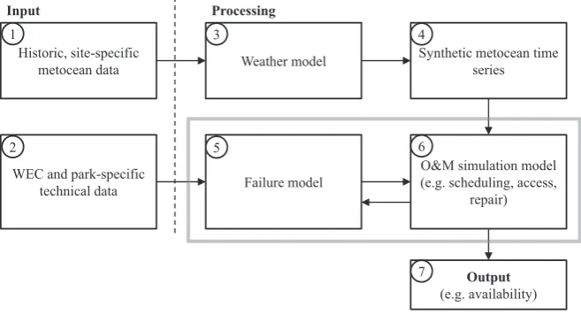
The purpose of the applied tool in its initial version was to investigate different maintenance strategies for large-scale offshore wind farms with a focus on accessibility. Modifications for the present study are made, as highlighted in the grey box of Fig. 1 , on the interaction between the failure modelling module ( 5 ) and the O&M simulation module ( 6 ); de- tails are provided in Fig. 2 . Further explanatory remarks are provided in the text below Fig. 1 .

Historic, site-specific metocean data

WEC and park-specific technical data

Weather model

Failure model

Synthetic metocean time series

O&M simulation model (e.g. scheduling, access,

repair)

Output (e.g. availability)

Input Processing

1

6 2

3 4

5

7

Fig.1. O&Msimulationtool– mainfunctionalities.

Running

Down

Mobilization & Logistics

Waiting for weather window

Transportation time

Repair time

Time

TTF-A Downtime TTF-B

5 6 5

Fig.2. FailuremoduleandO&Msimulationinteraction.

Medium-Range Weather Forecasts [31] . Wind speed and wave height time series from 22 years (1989 – 2010) have been used, providing a solid representation of conditions on site. A location in the East Anglia region – one of the largest offshore wind energy development sites – has been chosen as reference for this study. All metocean data used were available in six hour resolution.

Module 2 – WEC and park-specific technical data: all values pro- vided in Table 3 are included in the simulation in order to characterize the wind farm and turbines; the latter being further characterized by their component reliability – outlined in Table 1 and detailed in Section 3 . The turbines ’ power curve is linearized and used to quantify produc- tion losses due to downtime. Further details are omitted at this stage, as energy production is assessed as a time-based output parameter in this study.

Module 3 – weather model: data from the original source feeding Module 1 are used as an input to the applied weather model, whose functionality is based on a Markovian process, allowing for analysis of a large number of different yet realistic scenarios [32] . This feature is, in particular, important for modelling risk-related scenarios containing non-deterministic input and output variables – such as uncertain relia- bility numbers and distributions [33,34] . The Markov model generates discrete wave height time series for the desired length of simulation – here 20 years. Its functionality is based on the Markovian transition ma- trix, T_M, in which the transition probability of one wave height iturning into wave height jis specified by the parameter pij. The wave height state

Table1

Annualfailureratesandrepairtimesbaselinescenario.

System 𝜆low 𝜆medium 𝜆high Repairtime(h) Electricalsystem 0.285 0.570 0.855 12

Electroniccontrol 0.215 0.430 0.645 12 Sensors 0.125 0.250 0.375 12 Hydraulicsystem 0.115 0.230 0.345 18 Yawsystem 0.090 0.180 0.270 18 Rotorhub 0.085 0.170 0.255 24 Mechanicalbrake 0.065 0.130 0.195 18 Rotorblades 0.055 0.110 0.165 36 Gearbox 0.050 0.100 0.150 36 Generator 0.055 0.110 0.165 24 Support&housing 0.050 0.100 0.150 24 Drivetrain 0.025 0.050 0.075 24 Totalannualaverage 1.215 2.430 3.645

in the next time step depends solely on the wave height in the present time step – a property classifying the approach as a statistical process with finite memory. In order to account for weather seasonality, Markov matrices are developed for each month individually.

𝑇𝑀=

⎡ ⎢ ⎢ ⎢ ⎢ ⎣

𝑝11 𝑝12 ... 𝑝1𝑠 𝑝21 𝑝22 ... 𝑝2𝑠

... ... ... ...

𝑝𝑠1 𝑝𝑠2 ... 𝑝𝑠𝑠

⎤ ⎥ ⎥ ⎥ ⎥ ⎦

For each wave height bin, which has been discretized in 0.4 m steps, a cumulative distribution function (CDF) of observed wind speeds was obtained from the site-specific historic time series. During each time step, i.e. when a new wave height state is generated, a random number between zero and one is generated. The first value of the wind speed CDF that is greater than this number, is the chosen corresponding wind speed for the present time step.

Both synthetic wind speed and wave height time series generated by this weather model are validated by comparing them with observations. The validation encompasses both mean values but, most importantly for this application, also the persistence of weather phenomena [32] .

Module 4 – synthetic metocean time series: this module represents the output from Module 3, i.e. wind speed and wave height time series in six hour intervals over a timespan of 20 years.

Module 5 – failure model: from the basic technical information pro- vided in Module 2, the most relevant for this study are the components ’ FRs which are further processed to turbine faults at discrete time steps in Module 5. Failure rates were taken from [15] and have been varied to enable detection of failure distribution-specific mechanisms at different reliability levels. Three scenarios were considered: low, medium and high. The medium case represents annual FRs from the initial source; values were reduced or increased by 50 % for the low and high scenar- ios respectively. The chosen variations are at magnitudes enabling the detection of sensitivities. Considered systems, FRs and the correspond- ing assumed (fixed) repair times are shown in Table 1 . Failure rates are expressed by 𝜆; subscribed additions indicate the failure intensity in the three categories described before.

In time step zero, i.e. for simulation initialization, a time to failure (TTF) value is generated for each of the 12 systems on each modelled WEC (indicated by ‘TTF-A ’ in Fig. 2 ). The TTF is a discrete time step which is determined by the generation of a random number following a selected statistical distribution function around the failure. The selected statistical distribution function is treated as a parameter for the simu- lation studies introduced later. Further details of the failure modelling procedure are provided separately in Section 3 , as it forms the central element of the presented study.

If a turbine is not running due to a fault in one or more of the 12 subsystems, the demand for a repair activity is initiated (preventative activities or systems indicating an upcoming failure event are not con- sidered). Repair and replacement activities are treated equally within the scope of this paper, and summarized under the term ‘repair ’.

Module 6 – O&M simulation model: this module represents the cho- sen O&M strategy; the below descriptions focus on the decision tree followed subsequent to a fault of a system at one or more WECs. In case all assets are running without failure, the asset is fully available, thus not requiring any activity of the O&M fleet.

If a fault occurs, it is firstly checked if a crew and vessel suitable for the type of repair required is already on site; major components (ro- tor hub, rotor blades, gearbox, generator, support & housing and drive train) are hereby assumed to require a crane barge for repair – all other systems are assumed to require a crew transfer vessel. The absence of a suitable crew-vessel-combination on site leads to the activation of a vessel or crane barge located in the harbour, if any is available. The activated vessel or barge will pursue its transfer to the failed WEC as soon as weather conditions allow; restrictions relating to environmental conditions are limited to a certain wave height boundary, as further de- tailed in Section 4 . The deployment of vessels or crane barges is further restricted by the number and type of equipment available. This depends on the O&M fleet layout considered (summarized in Table 3 ). The max- imum time personnel are allowed to be offshore is considered as per the protection of labour laws. Assumed repair times are kept constant – their values, as provided in Table 1 , are estimated.

As soon as a failed system is up and running again (status is reached as soon as a crew-vessel-combination has been placed at the failed com- ponent for the allocated repair duration –Table 1 ), the next failure for this system is determined in the same way the initial TTF was generated

(indicated by ‘TTF-B ’ in Fig. 2 ). This procedure is repeated accordingly each time a failed component has been repaired, or replaced. It should be noted that system failures are not interrelated nor are they dependent on external conditions. The process of failure generation and repair is illustrated in Fig. 2 , in which the state of the component is either ‘run- ning ’ or ‘down ’.

Module 7 – outputs: relevant outputs are generated and may be used, depending on specific requirements; wind farm availability was chosen for the present study as it adequately combines the two issues of support- ability (here with a focus on accessibility) and reliability. Availability is calculated as time-based for the present study; production-based calcu- lations may also be applied. In particular for low availability values, one may expect that effects on economic performance are magnified if the latter method is applied [30] .

3. Failuremodelling

As briefly discussed in the previous section, failures are modelled as discrete events in time during simulation. Their number of occur- rences during a specified period of time depends on the FR 𝜆. If the FR of a component is two per year, the component will, in an infinite number of simulations, break twice a year on average. The FR is one of the key numbers used in reliability engineering and the correlation between component reliability and offshore wind farm availability has been observed and investigated in detail in previous studies [19,33] .

The pattern in which observed failures are distributed around a mean value differs from component to component. It depends on, e.g., physical characteristics of a component’s materials or external factors such as exposure to loading or corrosion. A methodology of collecting reliability data for FR predictions is provided in, amongst others, [16] .

Failure rates may be estimated based on existing track records (popu- lar examples are the WMEP and Offshore-WMEP by Fraunhofer [15,35] , or the SPARTA program by the OREcatapult [36] ) or model-based pre- dictions (e.g. by computer simulations providing the estimated fatigue lifetime of a structure using applicable standards such as [37] ). The ac- curacy of a FR estimate based on existing historical records strongly depends on the input data available: the more properly and consistently collected data points are available, the more accurate the estimate. It is of particular importance that the operating conditions as well as the asset class (referring to the comparability of technology applied) used for building up the database are comparable to the conditions the item will face in the operating environment of a planned application. The importance of the latter has been observed during the early years of the offshore wind industry in which, e.g., transformers applied in the Horns Rev I project were not insulated sufficiently for the offshore environ- ment, causing significant reliability issues [38] .

The accuracy of model-based FR predictions is highly dependent on the maturity of the modelling technique for the specific application under consideration. For instance, a simple loading on a single beam may be modelled very realistically. On the other hand, the uncertainty in modelling the physical behaviour of a newly developed gearbox in an offshore operating environment may be significantly larger. Both sources of uncertainty covered here, those of a statistical nature and those related to the modelling of system behaviour, must be treated in an adequate way; some methods are suggested in [39] .

A general term used for describing an item’s reliability characteris- tics is the time dependent reliability function R(t) which may also be referred to as the survival function. It describes the probability of an item to ‘survive ’, e.g. to be functional, at a certain time. This charac- teristic is explained by a simple example below, for which a fictitious failure record of an item is analysed. It should be noted that this exam- ple uses a Weibull distribution for providing the required theory for an understanding of the assumption of a constant FR.

Time No. of failures Observation Approximation TimeTime Probability [%] t: randomly chosen time step f(t): distribution function fitting the failure behaviour A 0

Fig.3. Histogramanddistributionfitoffictivefailuretrackrecord.

the applied mathematical descriptions. The details are omitted in the present paper but the reader may for example consult [40] for further information.

The TTF of the fictitious item is recorded. A simple histogram con- taining the number of failures in certain time intervals is developed. The histogram is then fitted with a suitable distribution function f(t) to enable a continuous description of the failure behaviour ( Fig. 3 ); the suitability of a chosen distribution function may be evaluated by a goodness of fit test procedure, such as the Chi-Square Method [41] , the Kolmogorov–Smirnov Test [40] , or Anderson–Darling Statistics [42] .

The reliability function of the item is then determined by deducting the area under the failure probability density function (PDF) until time step t from its total area (which always sums up to one). It may be expressed as follows (the following paragraph is interpreted with main inputs from [13] ):

𝑅(𝑡)=1−𝐴=1− ∫

𝑡

0 𝑓

(𝑡) (2)

The time dependent hazard rate 𝜆(t), representing the conditional probability of failure occurrence in the interval 0 to t, may be expressed by the following relation.

𝜆(𝑡)= 𝑓(𝑡)

𝑅(𝑡) (3)

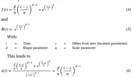
For PDFs which may be represented by a Weibull function, the single terms may be written as follows:

𝑓(𝑡)=𝛽 𝜂

(

𝑡−𝛾 𝜂

)𝛽−1

∗𝑒 (_{𝑡− 𝛾}

𝜂

)𝛽

(4)

and

𝑅(𝑡)= 𝑒 (_{𝑡− 𝛾}

𝜂

)𝛽−1

(5)

With:

𝑡 = Time 𝛾 = Offsetfromzero(locationparameter)

𝛽 = Shapeparameter 𝜂 = Scaleparameter

This leads to

𝜆(𝑡)= 𝛽 𝜂

(_𝑡

−𝛾

𝜂

)𝛽−1

∗𝑒 (_{𝑇− 𝛾}

𝜂

)𝛽

𝑒 (_𝑡−𝛾

𝜂

)𝛽−1 =𝛽_𝜂 (

𝑡−𝛾 𝜂

)𝛽−1

(6)

For the case of an exponential distribution, which is equal to a Weibull distribution with a shape parameter of one, the FR is constant and time independent:

𝜆(𝑡)= 1

𝜂 (7)

with

𝛽=1 (8)

Table2

DistributionfunctionsforTTFreproduction.

Distributionfunction Parameter1 Parameter2 Weibulldistribution Scaleparameter=1/𝜆 Shapeparameter=0.5 Weibull(Exponential) Scaleparameter=1/𝜆 Shapeparameter=1 Weibull(Rayleigh) Scaleparameter=1/𝜆 Shapeparameter=2 Weibull(Normal) Scaleparameter=1/𝜆 Shapeparameter=3.6 Betadistribution∗ _{Shapeparameter𝛼=0.2 Shapeparameter𝛽=0.2}

Betadistribution∗ _{Shapeparameter𝛼=0.4 Shapeparameter𝛽=0.4}

Betadistribution∗ _{Shapeparameter𝛼=0.8 Shapeparameter𝛽=0.8}

Uniformdistribution∗ _Lowerbound=0∗_{(1/𝜆) Upperbound=2}∗_(1/𝜆)

Fixedintervals∗∗ _{N/A N/A}

∗_{Avaluebetween0and1israndomlygeneratedfollowingthespecific}

distribu-tionfunctionandmultipliedbytwicetheinverseoftheFR

∗∗_{TheTTFisalwaysequaltothedeterministicinverseoftheFR.}

For the presented research, the mean value of the distribution func- tion describing failure occurrence probability corresponds to the FR ap- plied. It is constant throughout its lifetime but the shape of the respective function leads to higher failure probabilities in certain intervals (this de- pends on the function applied). This means that a modelled failure will, on average, occur according to its constant FR 𝜆but differ in the distri- bution around the average value (inverse of 𝜆).

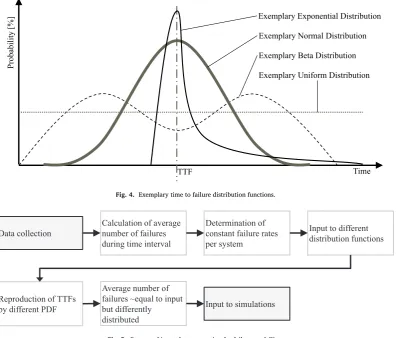
This is expressed graphically below in order to ease understanding ( Fig. 4 ). The figure shows a constant TTF and four exemplary differently shaped distributions: an exponential distribution, a normal and a beta distribution, as well as a uniform distribution (constant PDF). The mean TTF is equal for all four distributions but the probability density differs significantly.

It should be noted that distribution functions for failure modelling will optimally be based on existing observations – reference is made to the descriptions in [39] . Due to the fact that observations made in the industry so far are not following a clear pattern, failures are modelled in various different distributions. This represents the statistical uncertain- ties involved in reliability estimates which the industry is facing today and enables a view on the possible effects on asset performance resulting from those uncertainties.

The process from data collection to modelling of failures is sum- marized in Fig. 5 ; the top row from gathering input to provision of FRs is summarized in the works of Faulstich et al. [15] . The process shown in the lower row represents the work undertaken for generat- ing input parameters for the simulations within the scope of the present research.

Fig.4.Exemplarytimetofailuredistributionfunctions.

Fig.5. Processofinputdatagenerationforfailuremodelling.

Table 2 . Beta functions are used by generating a random number in an interval between zero and one which is following the respective dis- tribution.

The generated random number is subsequently multiplied by twice the inverse of the FR. This method generates two peaks of failure prob- ability (one close to zero and the other close to twice the inverse FR) – the form depending on the two parameters defining the shape of the function. The uniform distribution has been applied in a range of zero to twice the FR with equal probability of occurrence at all points within the respective interval. Furthermore, ‘fixed intervals ’ are applied for gener- ation of failures. This type reproduces failures at the exact TTF deter- mined by the inverse FR in a non-stochastic fashion – a scenario used in these studies to represent the most extreme case of failure accumulation, but with a low probability of occurrence in reality.

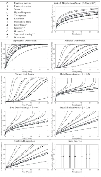
Cumulative distribution plots for each of the applied failure functions are provided in the graphs below for illustration; all plots are established by the generation of 100,000 random failures, applying the distribution function referred to within the failure modelling module of the simu- lation tool. The number of runs is selected in order to provide graphs showing a clear trend for each of the distribution types applied.

It should be noted that there are no drive train failures to be ex- pected when applying fixed intervals at a high reliability level, as the average TTF for this subsystem is 40 years and as such outside the life- time assumptions made for the wind farm modelled within the presented studies. As described before, this specific case is representing a scenario which is used for illustration of the most extreme case of failure accumu- lation, thus neglecting any stochastic behaviour such as the inclusion of outliers (the statistical significance of outliers should be tested in a more detailed study of data collection). Such phenomena are covered within the other eight distribution types, enabling analysis of particularities for both deterministic and stochastic variables.

A graphical representation of the contents discussed above is pro- vided in Fig. 6 (a legend, also applicable for all other figures presented, is at the top left).

∗_/ ∗∗_{subsystems have the same FR, i.e. the same distribution function}

in the figures below.

Within each simulation run, all component FRs are modelled with the same distribution. This amplifies the effect, thus enabling a clearer recognition of distribution-specific mechanisms and results; the true physical behaviour may therefore only be represented for a certain set of subsystems as certainly not all components will follow the same failure distribution throughout their lifetime.

The application of component-specific failure distribution functions is desirable and proposed for future works. The feasibility of such stud- ies would require far more asset- and site-specific reliability data, as outlined at the beginning of this section.

4. Baselinescenario

All scenarios analysed for this study were run under the same basic conditions; the chosen parameters as summarized in Table 3 are repre- sentative of a modern offshore wind farm in European waters. Parame- ters changed are the distribution function for the generation of pseudo- random TTF values during simulation as well as the general reliability level represented by the mean TTF values applied (inverse of FR pro- vided in Table 1 ).

Electrical system Electronic control Sensors

Hydraulic system Yaw system Rotor hub Mechanical brake Rotor blades* Gearbox** Generator*

Support & housing** Drive train

Weibull Distribution (Scale: 1/λ Shape: 0.5)

Exponential Distribution Rayleigh Distribution

Normal Distribution Beta Distribution (α = β = 0.2)

Beta Distribution (α = β = 0.4) Beta Distribution (α = β = 0.8)

Uniform Distribution Fixed Intervals

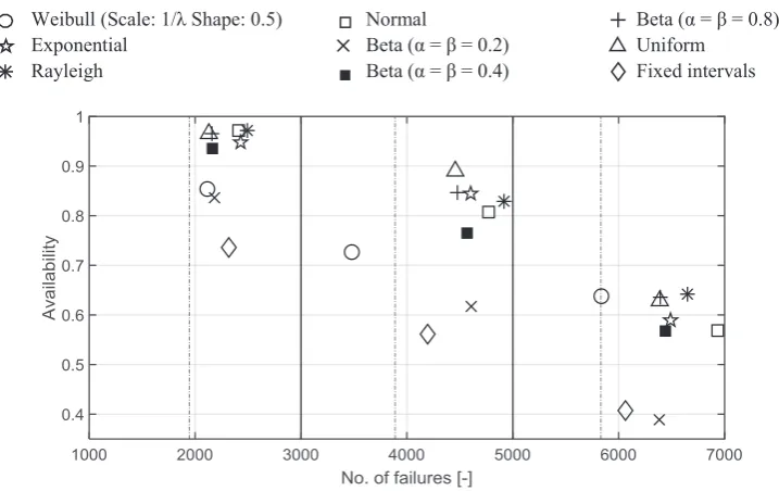
Fig.7. Availabilityvs.totalno.offailures– overview.

Table3

Siteconditionsbaselinescenario.

Parameter Value

Site UKeastcost(EastAngliaregion) Meanwindspeedathubheight 7.9m/s

Meanwaveheight 1.51mHs(significantwaveheight) Numberofturbines 80

Ratedpower 5MW Totalcapacity 400MW Lifetime 20years Numberofvessels 3 Numberofcranebarges 1 Wavebearingcapacityvessel 2.2m Wavebearingcapacitycranebarge 2.2m Transittimevessel 6h Transittimecranebarge 12h

tions considering 20 operating years have been carried out in order to generate representative results. In the interest of accounting for the po- tentially overlapping effects of stochasticity of weather and failure mod- ules, the results are presented under deterministic weather conditions in a comparative study separately in Section 6 .

5. Results

The main results obtained from the simulations are presented within the following section. Starting from a top level overview summarizing the main mechanisms, more detailed phenomena are discussed subse- quently. Critical interpretation and classification of the studies ’ results are concluded in a separate section closing the paper.

Fig. 7 provides a global view of wind farm availability levels ver- sus the average number of failures during each modelled scenario; the number of failures are provided due to the probabilistic characteristics of the applied failure generator resulting in the actuality that, depend- ing on the distribution applied, some generated failures are occurring at a time later than the total simulation duration of 20 years. Truncated distribution functions were not applied as the parameters in the distribu- tion functions were tuned to deliver a constant average FR. All numbers provided are to be understood as the average of ten simulations. The expected number of failures per scenario is to be calculated according to Table 1 ( 𝜆being the annual FR).

𝑁𝑜.𝑜𝑓𝑓𝑎𝑖𝑙𝑢𝑟𝑒𝑠=𝜆∗80𝑡𝑢𝑟𝑏𝑖𝑛𝑒𝑠∗20𝑦𝑒𝑎𝑟𝑠 (9)

Table4

Availabilityvs.failurerateanddistributiontype. Availability

LowFR MediumFR HighFR 1 Weibull(Scale:1/𝜆Shape:0.5) 0.85 0.73 0.64 2 Exponential 0.95 0.84 0.59 3 Rayleigh 0.97 0.83 0.64 4 Normal 0.97 0.81 0.57 5 Beta(𝛼=𝛽=0.2) 0.84 0.62 0.39 6 Beta(𝛼=𝛽=0.4) 0.94 0.76 0.57 7 Beta(𝛼=𝛽=0.8) 0.97 0.85 0.64 8 Uniform 0.97 0.89 0.63 9 Fixedintervals 0.74 0.56 0.41 Meanavailability 0.91 0.77 0.56

This relation results in a number of expected failures in each cate- gory: 1944 in the low FR region, 3888 in the medium FR region and 5832 in the high FR region. These values are illustrated by dash-dotted vertical lines in Fig. 7 .

Fig. 7 is split into three regions, representing an increase in FR from the left (low FR) and middle (medium FR) to the right (high FR). Each marker represents one scenario at the respective reliability level; the markers are allocated to the distribution functions in the following order.

A general downward trend in availability with an increasing number of failures is observed in the graph above; as expected and described pre- viously, this behaviour represents the direct correlation between num- ber of failures and wind farm availability. From Fig. 7 it can also be seen that the number of failures is generally over-predicted in the ap- plied failure module. The Weibull distribution, with a shape parameter of 0.5 and fixed failure intervals, delivers the values closest to the ex- pected. Applying a Beta distribution with both shape factors at a value of 0.8 delivers comparable results to a uniform distribution, with a very high correlation in low and high FR regions.

Table5

Failuretounavailabilityratiofordifferentfailureratesanddistributiontypes. FUR/rank

LowFR MediumFR HighFR 1 Weibull(Scale:1/𝜆Shape:0.5) 146 /7 127 /7 161 /4 2 Exponential 467 /5 296 /2 158 /6 3 Rayleigh 869 /1 288 /4 186 /1 4 Normal 853 /2 247 /5 161 /5 5 Beta(𝛼=𝛽=0.2) 133 /8 120 /8 104 /8 6 Beta(𝛼=𝛽=0.4) 334 /6 195 /6 149 /7 7 Beta(𝛼=𝛽=0.8) 630 /3 291 /3 176 /2 8 Uniform 608 /4 404 /1 172 /3 9 Fixedintervals 88 /9 96 /9 102 /9

The number of failures generated in each of the scenarios is not con- stant. This is due to the fact that the applied distribution functions were adjusted to deliver the correct mean FR, considering an infinite number of runs. The inherent consequences are over- and under-productions of failures in certain intervals, considering non-truncated distribution func- tions. In order to make results comparable, a value normalizing avail- ability with the number of failures is introduced. The factor chosen here represents the number of component failures leading to a loss of 1 % in availability –referred to as FUR (failure to unavailability ratio).

The FUR has been developed as part of the presented studies and has, to the authors ’ knowledge, not been applied in other studies. It is deemed an appropriate measure to evaluate results and further enables a reduction in the simulation outcomes to a quantified measure repre- senting the core of the investigation.

𝐹𝑎𝑖𝑙𝑢𝑟𝑒𝑡𝑜𝑢𝑛𝑎𝑣𝑎𝑖𝑙𝑎𝑏𝑖𝑙𝑖𝑡𝑦𝑟𝑎𝑡𝑖𝑜(𝐹𝑈𝑅)= 𝑁𝑜.𝑜𝑓𝑓𝑎𝑖𝑙𝑢𝑟𝑒𝑠

(1−𝐴𝑣𝑎𝑖𝑙𝑎𝑏𝑖𝑙𝑖𝑡𝑦)∗100 (10)

The results for each distribution function at the three applied relia- bility levels are summarized below. From the values presented, a scoring may be derived with the ‘most favourable ’ failure distribution being the one for which the least percentage of downtime is caused per failure. Such an evaluation was performed with the results obtained in the sim- ulations.

Table 5 shows the FUR for each distribution and at each reliability level. The rank, according to favourability, stands next to the FUR value in the summary table ( Table 5 ).

It can be seen that the favourability of a distribution varies with reli- ability, meaning that the most favourable distribution is not a constant at different reliability levels. In order to account for that, an average ranking has been calculated for each distribution (e.g. the Rayleigh dis- tribution is scoring an average of ( 1 +1 +4)/3 =2 which is the lowest overall count and therefore the most favourable distribution considering equal weighting of each reliability level).

Beta ( 𝛼=𝛽=0.8) and Uniform, Normal and Exponential as well as Weibull (Scale: 1/ 𝜆Shape: 0.5) and Beta ( 𝛼=𝛽=0.4) distributions show the same average ranking and are therefore sharing the same score in the overall ranking as summarized below.

1.Rayleigh 3.Normal 4.Beta(𝛼=𝛽=0.4) 2.Beta(𝛼=𝛽=0.8) 3.Exponential 5.Beta(𝛼=𝛽=0.2) 2.Uniform 4.Weibull(Scale:1/𝜆Shape:0.5) 6.Fixedintervals

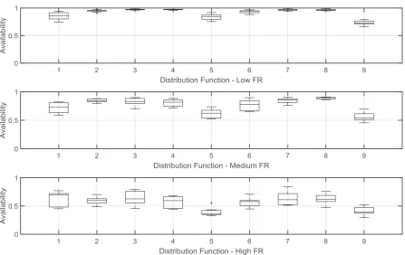
A graphical representation of the results is provided in Fig. 8 . Looking at the results, one may conclude that respecting not only pure average FRs but also their distribution is inevitable for efficient offshore wind farm O&M. Expanding on that, it is further important to consider the amount of variability in availability estimates to be ex- pected.

The graphs in Fig. 9 show the results from each run in each param- eter set investigated. This results in ten runs being represented in the boxplot, with the centre line representing the set’s median and the up- per and lower box boundaries the 75th and 25th percentile. The outer whiskers are reaching to +/ −2.7 standard deviations of the respective set of results, meaning that less than 1% of the expected values should

Table6

Standarddeviationofavailabilitiesatdifferentreliabilitylevelsanddistribution types.

Standarddeviation

LowFR MediumFR HighFR 1 Weibull(Scale:1/𝜆Shape:0.5) 0.072 0.086 0.120 2 Exponential 0.022 0.028 0.065 3 Rayleigh 0.008 0.060 0.121 4 Normal 0.007 0.060 0.099 5 Beta(𝛼=𝛽=0.2) 0.051 0.077 0.069 6 Beta(𝛼=𝛽=0.4) 0.027 0.092 0.080 7 Beta(𝛼=𝛽=0.8) 0.013 0.045 0.111 8 Uniform 0.013 0.017 0.090 9 Fixedintervals 0.039 0.080 0.074 Meanstandarddeviation 0.028 0.061 0.092

lie outside the box. The vertical axis shows the availability and the hori- zontal axis the distribution type applied, in accordance with the follow- ing order. The top figure represents results for high, the middle figure for medium and the bottom figure for low reliability.

1 Weibull(Scale:1/𝜆Shape:0.5) 4 Normal 7 Beta(𝛼=𝛽=0.8) 2 Exponential 5 Beta(𝛼=𝛽=0.2) 8 Uniform 3 Rayleigh 6 Beta(𝛼=𝛽=0.4) 9 Fixedintervals

A significant increase in variability of results with decreasing relia- bility can be observed for all distribution functions under investigation. This is expressed in terms of the standard deviation of availabilities ob- served in each of the ten different runs considered for each scenario given in Table 6 .

From the data presented above, it can be seen that the mean stan- dard deviation of expectable wind farm availabilities is approximately doubling for an increase of FR by a factor of two and tripling at an in- crease of three, when averaging all the results at each reliability level. This correlation is illustrated in Fig. 10 based on the data presented in Table 6 .

The expected variability of performance, depending on the reliabil- ity level, becomes particularly important for assets for which reliability numbers are highly uncertain; namely those with a very limited track record of proven technology under the respective operating conditions, or those relying on the application of novel technology. For a guidance to classify and consider the novelty of technologies in that respect, read- ers are referred to [43] .

6. Semi-probabilisticcomparisonstudy

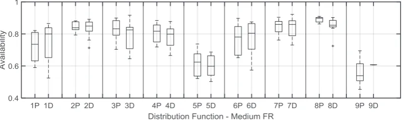
As mentioned above, it has been decided to keep the requirement for stochasticity in the weather module as well as in the failure module as this realistically represents the actual conditions and sources of uncer- tainty offshore. In order to avoid overlapping influences of stochasticity, a comparative study was conducted investigating the impact of differ- ent failure distributions on the farm’s availability figures, considering deterministic weather conditions only (the same synthetic wind speed and wave height time series was applied for all cases). The compara- tive study has been performed at medium reliability level, considering input values from the initial source [15] . Results of this study are con- cluded below. Corresponding to the data presented in Fig. 9 , the num- bers provided below refer to the type of distribution function applied; the supplement ‘P ’ or ‘D ’ next to the number stands for probabilistic or deterministic weather respectively.

1 Weibull(Scale:1/𝜆Shape:0.5) 4 Normal 7 Beta(𝛼=𝛽=0.8) 2 Exponential 5 Beta(𝛼=𝛽=0.2) 8 Uniform 3 Rayleigh 6 Beta(𝛼=𝛽=0.4) 9 Fixedintervals

Fig.8. Failuretounavailabilityratiofordifferentfailureratesanddistributiontypes.

Fig.9. Failuredistribution-specificavailabilitiesforthreereliabilitylevels.

Fig.10. Standarddeviationofavailabilitiesatdifferentreliabilitylevels.

are simulated fully deterministically (fixed failure intervals and deter- ministic weather time series) is demonstrating the influence of weather stochasticity clearly. The variations in results between run 9P and 9D are solely due to weather stochasticity (as fixed TTF values are a determinis- tic number, even in the probabilistic run); nevertheless, the mean values

of the results are at a comparable level for all distribution functions ex- cept in the case of fixed failure intervals, the latter being included for the purpose of assessing results of an extreme and unrealistic case. It is therefore concluded that this comparative study provides confidence in the validity of the results generated in the fully probabilistic model. Due to the clear patterns observed in the results as illustrated in Fig. 11 , it is expectec that characteristics are comparable at other reliability levels.

7. Discussion

Fig.11. Probabilisticvs.semi-probabilisticsimulationresults.

project phases, with the potential to finally contribute significantly to the de-risking of investments in offshore wind projects.

The authors see different ways leading to an understanding of time- and condition-dependent failure intensities. The starting point is the in- vestigation of a component’s physical behaviour in its operational en- vironment. Corresponding failure modes and mechanisms must be un- derstood to the highest possible degree. This may be achieved by (i) studying operating track records of existing assets in more detail, (ii) in- depth physical testing of new equipment, enabling the understanding of expectable failure behaviour, and (iii) improving modelling techniques to allow for more accurate model-based estimates if physical testing is not feasible. Several attempts are currently being made in industry and academia to improve the above-mentioned points, potentially allowing the incorporation of new knowledge into maintenance simulation mod- els but also the development of measures allowing for efficient predic- tive maintenance strategies, such as condition monitoring systems. Self- learning techniques, as applied in neural networks, may support this by their inherent ability to translate operating experience into improved strategies during operation.

As soon as the maintenance demand can be predicted more accu- rately, the setup of O&M organizations may be re-evaluated to fit the ex- pected requirements. If, for example, large failure accumulations are ex- pected, the introduction of a flexible fleet should be considered. Larger operators may consider a portfolio optimized O&M setup; others might make use of sharing options. Technical modifications, such as implemen- tation of redundant or high performance materials, may be considered if components show undesired reliability characteristics.

The contents of the present paper are model-based and thus inher- ently subject to simplification. Care has been taken to ensure that the extent of the simplification is at a level that does not compromise the validity of the major messages concluded. Simplifications made are re- lated to the modelling process and computational efforts. Even though the number of simulated turbine operating years (16,000 per scenario) is significant, the probabilistic nature of the simulation process could po- tentially profit from more. Analysed availability figures are the average taken from ten simulations of 20 years of operation. Statistical variance may be reduced in a larger amount of runs, resulting in a stronger con- fidence in respect to convergence observations. A comparative study under semi-probabilistic conditions was performed to enhance confi- dence in the results. Indeed, this study indicates that the impact of the stochasticity of the weather module does not have a great influence on the trends observed in the obtained results.

The main simplifications made regarding the model itself are related to the points listed below. All of them should be considered to enhance accuracy and are subject to future work. The simplifications are not expected to impact on the conclusions presented here but will influence the validity of the results in terms of absolute numbers (the trend of changing availabilities will remain but the actual availability value will be closer to reality when considering model updates).

• Considered failure distributions are based on literature. They do not necessarily represent the real physical behaviour of a component

• Failures of components are not intentionally interrelated. Even though this is inherently respected in the baseline data, the failure modelling module does not force interrelated failures

• Position-specific particularities are not considered. Components of a turbine being subject to, e.g., excessive turbulence, are as likely to fail as if they were built into any other turbine in the park

• Preventive maintenance activities potentially avoiding or delaying failures as well as condition monitoring systems indicating develop- ing faults, are not included. As both will play a more significant role in the future, this will be included in further research

• The model does rely on crew transfer vessels and crane barges. Fu- ture work should respect helicopter access and large service opera- tion vessels (SOVs)

• Day and night-time as well as visibility restrictions due to fog are not considered. This will be important, in particular for the incorpo- ration of helicopter access

• Time resolution for the simulation process is six hours. In order to be able to investigate for greater detail, this may be adjusted.

8. Conclusions

The core motivation of the presented research was to understand the implications of statistical uncertainty of offshore wind turbine reliability estimates on asset performance.

Results show that offshore wind farm performance depends not only on absolute reliability figures (failure rates) but in equal measure on the way failures are distributed around a mean value. The impact of the latter is significant and its implications are relevant to a wide range of stakeholders in the industry – from financial bodies to wind farm developers and operators.

Adequate consideration of component failure behaviour is vital for future developments in the field, with an emphasized importance in respect to large scale projects and turbine classes beyond the 10 MW benchmark.

Both, statistical uncertainty due to a lack of publicly available re- liability data, as well as modelling uncertainty due to application of new technology such as the application of floating wind turbines, must be addressed in order to leverage the investment de-risking potential available today.

The consideration of the results presented in this paper in future O&M simulation tools is a feasible next step enabling more accurate scenario modelling; leading to more precise forecasts of technical per- formance and the consequential potential for improvements in achieve- ment of financial targets.

Acknowledgements

References

[1] CorbettaG,HoA,PinedaI,RubyK.Windenergyscenariosfor2030.EuropeanWind EnergyAssociation;2015.

[2] MocciaJ,WilkesJ,PinedaI,CorbettaG.Windenergyscenariosfor2020.European WindEnergyAssociation;2014.

[3] DaveyE,NimmoA.Offshorewindcostreduction– pathwaysstudy.TheCrown Estate;2012.

[4] GovernmentHM.Offshorewindindustrialstrategy– businessandgovernment ac-tion.OWIC(OffshoreWindIndustryCouncil),OWPB(OffshoreWindProgramme Board),UKGovernment;2013.

[5] LetterbyIndustryLeaders.Offshorewindcanreducecoststobelow€80/MWhby 2025, https://windeurope.org/wp-content/uploads/files/policy/topics/offshore/ Offshore-wind-cost-reduction-statement.pdf;2016[accessed11.08.2016]. [6] KemptonW,McClellanS,OzkanD.Massachusettsoffshorewindfuturecoststudy.

UniversityofDelaware;2016.

[7] TechnologyInnovationNeedsAssessment(TINA).Offshorewindpowersummary report.LowCarbonInnovationCoordinationGroup;2012.

[8] RubelH,PaulsenK,HeringG,WaldnerM,ZenneckJ.EU2020offshore-windtargets – the€110billionfinancingchallenge.TheBostonConsultingGroup;2013.

[9] MadlenerR,SiegersL,Bendig S.Risikomanagementund–controlling bei Off-shore– Windenergieanlagen.ZfEZeitschriftfürEnergiewirtschaft2009;33(February (2)):135–46.

[10]ProskovicsR,HuttonG,TorrR,ScheuM.Methodologyforriskassessmentof float-ingwindsubstructures.In:Proceedingsofthe13thdeepseaoffshorewindR&D conference,Trondheim.EERADeepWind;2016.

[11]RamB.Assessingintegratedrisksofoffshorewindprojects:movingtowards gigawat-t-scaledeployments.WindEng2011;35(3):247.

[12]EN13306:2010(E).Maintenance– maintenanceterminology.EuropeanCommittee forStandardization;2010.

[13]FinkelsteinM.Failureratemodellingforreliabilityandrisk,London:Springer;2008. ISBN978-1-84800-985-1.

[14]LevinM,KalalT.ImprovingproductReliability:strategiesandimplementation,West Sussex:Wiley;2003.ISBN0-470-85449-9.

[15]FaulstichS,HahnB,TavnerPJ.Windturbinedowntimeanditsimportancefor off-shoredeployment.WindEnergy2011;14:327–37.

[16]EchavarriaE,HahnB,BusselGJW,TomiyamaT.Reliabilityofwindturbine tech-nologythroughtime.JSolarEnergyEng2008;130.

[17]TavnerPJ,XiangJ,SpinatoF.Reliabilityanalysisforwindturbines.WindEnergy 2007;10:1–18.

[18]WilkinsonM,etal.Methodologyandresultsofthereliawindreliabilityfieldstudy. In:ProceedingsoftheEuropeanWindEnergyConference(EWEC),Warsaw;2010.

[19]CarrollJ,McDonaldA,McMillanD.Failurerate,repairtimeandunscheduledO&M costanalysisofoffshorewindturbines.WindEnergy2015;19(6):1107–19.

[20]FengY,TavnerPJ,LongH.EarlyexperienceswithUKRound1offshorewindfarms. ProcInstCivilEng2010;163(4):167–81.

[21]OdgaardPF,StoustrupJ.Abenchmarkevaluationoffaulttolerantwindturbine controlconcepts.IEEETransControlSystTechnol2015;23:1221–8.

[22]Siegel D,ZhaoW,LapiraE,AbuAli M,LeeJ.Acomparative studyon vibra-tion-basedconditionmonitoringalgorithmsforwindturbinedrivetrains.Wind En-ergy2014;17(5):695–714.

[23]Tautz-WeinertJ,WatsonSJ.UsingSCADAdataforwindturbinecondition monitor-ing– areview.IETRenewablePowerGeneration;2016.ISSN1752-1416.

[24]ScheuM,MathaD,HofmannM,MuskulusM.Maintenancestrategiesforlarge off-shorewindfarms.EnergyProcedia2012;24:281–8.

[25]HofmannM.Areviewofdecisionsupportmodelsforoffshorewindfarmswithan emphasisonoperationandmaintenancestrategies.WindEng2011;35(1):1–16.

[26]DinwoodieI,EndrerudOEV,HofmannM,MartinR,SperstadIB.Referencecases forverificationofoperationandmaintenancesimulationmodelsforoffshorewind farms.WindEng2015;39(1):1–14.

[27]ZitrouA,BedfordT,DaneshkhahA.Robustnessofmaintenancedecisions: Uncer-taintymodellingandvalueofinformation.ReliabEngSystSaf2013;120:60–71.

[28]SanchezA,CarlosS,MartorellS,VillanuevaJF.Addressingimperfectmaintenance modellinguncertaintyinunavailabilityandcostbasedoptimization.ReliabEngSyst Saf2009;94:22–32.

[29]NannapaneniS,MahadevanS.Reliabilityanalysisunderepistemicuncertainty. Re-liabEngSystSaf2016;155:9–20.

[30]ScheuM.MaintenancestrategiesforlargeoffshorewindfarmsDiplomathesis;2012.

[31]EuropeanCentreforMedium-RangeWeatherForecasts.ERA-interimdatasets,www. ecmwf.int/en/research/climate-reanalysis/era-interim;[accessed2.01.2016]. [32]ScheuM,MathaD,MuskulusM.ValidationofaMarkov-basedweathermodelfor

simulationofO&Mforoffshorewindfarms.In:Proceedingsofthe22ndinternational offshoreandpolarengineeringconference;2012463-368.

[33]NielsenJJ,SørensenJD.Onrisk-basedoperationandmaintenanceofoffshorewind turbinecomponents.ReliabEngSystSaf2011;96:218–29.

[34]ToledoMLG,FreitasMA,ColosimoEA,GilardoniGL.ARAandARIimperfectrepair models:Estimation,goodness-of-fitandreliabilityprediction.ReliabEngSystSaf 2015;140:107–15.

[35]Fraunhofer Institut. Information websiteon WInD-Pool,http://wind-pool.iwes. fraunhofer.de/wind_pool_de/WInD-Pool/[accessedon21.09.2016].

[36]OffshoreRenewableEnergyCatapult– OREC.InformationwebsiteonSPARTA pro-gram, https://ore.catapult.org.uk/our-knowledge-areas/operations-maintenance/ operations-maintenance-projects/sparta/[accessedon21.09.2016].

[37]DNV-GLRecommendedPractice– DNVGL-RP-C203.Fatiguedesignofoffshoresteel structures.DNVGL;April2016.

[38]NewsArticle.HornsRevrevealstherealhazardsofoffshorewindOctober2004.

[39]DNVClassificationNoteNo.30.6.Structuralreliabilityanalysisofmarinestructures. DetNorskeVeritas;July1992.

[40]O’ConnorPDT,KleynerA.Practicalreliabilityengineering.5thed.WestSussex: Wiley;2013.ISBN978-0-470-97982-2.

[41]GreenwoodPE,NikulinMS.Aguidetochi-squaredtesting,WestSussex:WileySeries inProbabilityandStatistics;1996.ISBN978-0-471-55779-1.

[42]WeissteinE.Encyclopaediaofmathematics– SupplementVolumei.Kluwer Aca-demicPublishers;1997.ISBN0-7923-4709-9.