City, University of London Institutional Repository
Citation
:
Bishop, P. G. and Cyra, L. (2012). Overcoming non-determinism in testing smart devices: how to build models of device behaviour. Paper presented at the 11th International Probabilistic Safety Assessment and Management Conference and the Annual European Safety and Reliability Conference 2012 (PSAM11 & ESREL 2012), 25 - 29 June 2012, Helsinki, Finland.This is the unspecified version of the paper.
This version of the publication may differ from the final published
version.
Permanent repository link:
http://openaccess.city.ac.uk/2464/Link to published version
:
Copyright and reuse:
City Research Online aims to make research
outputs of City, University of London available to a wider audience.
Copyright and Moral Rights remain with the author(s) and/or copyright
holders. URLs from City Research Online may be freely distributed and
linked to.
City Research Online: http://openaccess.city.ac.uk/ [email protected]
Overcoming Non-determinism in Testing Smart Devices:
How to Build Models of Device Behaviour
Peter G. Bishopab*, Lukasz Cyrac
a
Centre for Software Reliability, City University, London, United Kingdom
b
Adelard LLP, London, United Kingdom
c
European Commission Joint Research Centre, IPSC, Security Technology Assessment Unit, Ispra, Italy
Abstract: Justification of smart instruments has become an important topic in the nuclear industry. In practice, however, the publicly available artefacts are often the only source of information about the device. Therefore, in many cases independent black-box testing may be the only way to increase the confidence in the device. In this paper we provide a set of recommendations, which we consider to be the best practices for performing black-box assessments. We present our method of testing smart instruments, in which we use the publicly available artefacts only. We present a test harness and describe a method of test automation. We focus on the analysis of test results, which is made particularly complex by the inherent non determinism in the testing of analogue devices. In the paper we analyse the sources of non-determinism, which for instance may arise from inaccuracy in an analogue measurement made by the device when two alternative actions are possible. We propose three alternative ideas on how to build models of device behaviour, which can cope with this kind of non-determinism. We compare and contrast these three solutions, and express our recommendations. Finally, we use a case study, in which a black box assessment of two similar smart instruments is performed to illustrate the differences between the solutions.
Keywords: Smart Sensor, Testing, Non-Determinism, Test Automation.
1. INTRODUCTION
Smart instruments have operational and safety benefits as they are more accurate and require less calibration, but since they are programmable devices, there is a potential for software defects within the device, which could result in unpredictable behaviour. Nonetheless, smart instruments have been successfully used in many industries and some of the devices available on the market have hundreds of thousands of hours of operational experience. This makes them very attractive for the nuclear industry, but for safety related purposes additional safety justification and evidence often needs to be developed (Bishop et al., 2005). Unfortunately, in many cases the manufacturers are not willing to share their development documentation with their clients, and the only way to develop additional evidence is to perform an assessment using the publicly available artefacts solely, e.g. the user manuals for operation and maintenance and the device itself. We call this kind of assessment a black-box assessment.
The primary part of the black-box assessment is functional, statistical testing. To gain sufficient confidence in the smart device functionality, hundreds of thousands of test cases need to be performed, so the test execution and result analysis must be automated.
2. TEST AUTOMATION
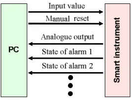
Smart instruments can implement a range of different functions. They typically make measurements using either analogue or digital interfaces, perform some form of computation and output processed values through analogue outputs, digital outputs or relays. Smart devices can generally be configured to make adjustments to processing function that is preformed.
[image:3.612.195.415.164.245.2]This paper describes the testing of a typical smart device, namely a programmable alarm, the main features of which are shown in Figure 1.
Figure 1. Model of smart instrument
This smart instrument has several alarm outputs and each alarm output controls a relay.
− Each alarm can be configured independently.
− The alarms can be configured to operate when the value exceeds or is below a certain limit. We call them respectively trip point high and low alarms.
− The alarm trip point is configurable.
− Alarms have configurable deadbands, to avoid “jitter”. Once the alarm is activated, it is only turned off when the input value moves outside the deadband region.
− Alarms have configurable delays, i.e. the value must remain in the alarm range for a certain amount of time to trigger the alarm.
− Alarms can be latching and non-latching, i.e. once set they do or do not require a manual reset. The test environment used to automate the tests consisted of three separate elements:
1. An off-line test data generator, which generates a file with test cases.
2. An on-line test execution system, which takes the file specifying the test cases and generates a file containing the test cases and the corresponding test results.
3. An off-line result checker, which takes the result file and detects discrepancies between the test results and the model of behaviour it uses.
This design makes it possible to:
− Use different types of test generator, such as direct plant measurements, simulators, or specification derived tests
− Execute the device tests only once (a very time consuming part of the process)
− Analyse the test results stored in a file many times using different versions of the result checker. For example a flaw in the checker can be fixed and the results rechecked without performing more tests on the physical device
− Furthermore, this design makes it possible to rerun exactly the same sequence of tests many times to check, e.g. if the identified discrepancies are repeatable.
We recommend splitting the test harness into three elements as presented above.
[image:3.612.239.373.614.716.2]We implemented the off-line test generator as a Java application which generates transients, i.e. signals starting at a random level below the trip point, then rising with a random slope to a random value above the trip point, and decreasing back with a random slope to a random value below the trip point. Also noise was added to the signal. We recommend adding noise to test signals as “the most interesting” situations happen when the input changes slightly around the trip point.
The model of the on-line test execution system is presented in Figure 2. We implemented it as a LabView application. The application executes the test cases in a cycle. As we did not use a real time operating system, but a generic purpose one, we experienced occasionally “unexpected” delays in the execution. This is not a problem if we know when the delay happens and how long it takes. Therefore, our test result file includes both test results and detailed time readings. In practice this means taking a sequence of readings as follows: record the time – read a new test case from the file – record the time – send a new input to the device – record the time – wait x seconds – etc. We recommend taking time readings after every micro-step of the execution so that once we detect a delay we know exactly when it occurred.
Finally, we implemented the off-line result checker. This application has a built in model of behaviour of the device. This apparently straightforward task is more complicated than it first appears (Bishop and Cyra, 2010) as the device can generate different, but equally valid responses to the same test input sequence. The causes of the non-deterministic behaviour, and alternative means of checking the tests in the presence of non-determinism are discussed in detail in the following sections of this paper.
3. NON-DETERMINISM
Non-determinism is unavoidable in testing analogue devices. It arises from a number of different sources:
− Smart device accuracy − Smart device sampling rates
− Smart device response lags
− Lack of knowledge about the internal design of the device
− Inaccuracy of the test harness.
3.1. Smart device accuracy
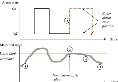
The input provided to the smart device is read with certain accuracy. This leads to non-determinism when the input value is close to a decision point, e.g. an alarm trip point, as presented in Figure 3. The measurement inaccuracy is represented by the thick grey line (1). If the input is close to the limit (2) we cannot know whether the alarm was set on or not, which means that two alternative alarm states are possible (3). This situation, in turn, leads to non determinism in the following part of the diagram (4), as the state of the alarm depends on its state in the past. Finally, the state of the alarm becomes deterministic again once we are sure that the input value left the deadband (5).
3.2. Smart device sampling rates
The input provided to the smart device is sampled using a certain sampling rate, as presented in Figure 4. Two alternative ways of taking samples are presented using solid (1) and dashed (2) lines. Depending on the way of sampling used the device will or will not notice the short excursion of the input above the alarm limit (3). This means that the output will be non deterministic (4) until the input value is definitely outside the deadband region (5).
Alarm state Off On Measured input Alarm Limit Deadband Time Non-deterministic value Either alarm state possible Time 1 2 4 5 3
Figure 3. Non-determinism due to inaccuracy
Alarm state Off On Measured input Alarm Limit Deadband Time
[image:4.612.323.525.403.544.2]Smart device input sample interval Either alarm state possible Time 1 2 3 4 5
3.3. Smart device response lags
There is uncertainty about when the expected response will appear at the smart device output. This is illustrated in Figure 5.
When the input exceeds the limit (1) we expect the alarm to be set on. This, however, can happen almost immediately (2) or with a certain delay (3), which is usually defined in the user manual as the maximal response time of the device. So for a certain period of time the output is non-deterministic.
Alarm state Off On Measured input Alarm Limit Deadband Time
Smart device input sample interval Either alarm state possible Time Output response lag(s) 1
[image:5.612.322.518.70.202.2]2 3
Figure 5. Non-determinism due to response lags
3.4. Lack of knowledge about internal design of device
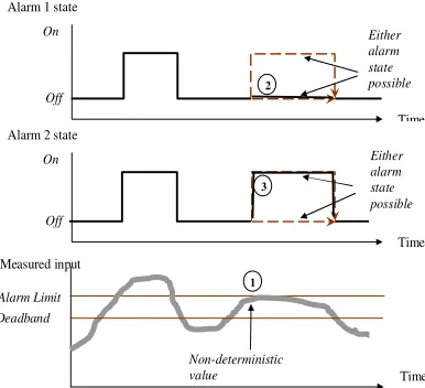
Furthermore, when we consider the device as the whole, with the analogue output and several relays it may turn out that we do not know enough about the internal design of the device to know what the correct output in a certain situation is.
In Figure 6 we see a non-deterministic output caused by the inaccuracy of the input value (1). There are two alarms that have identical configuration settings. The question is whether the alarm 1 activation state (2) can be different from the alarm 2 state (3). As we do not know the internal design of the device (e.g. there could be a different processor for each alarm), we have to accept inconsistent alarms as a legitimate result.
Alarm 2 state
Off On Measured input Alarm Limit Deadband Time Non-deterministic
value Time
1 3
Alarm 1 state
Off On Time 2 Either alarm state possible Either alarm state possible
Figure 6. Uncertainty about internal design
3.5. Inaccuracy of test harness
Finally, the test harness introduces additional determinism to the measurement. It increases the non-determinism by:
(1) increasing the inaccuracy of the input value by generating inaccurate test signals, (2) increasing the inaccuracy of the output value by recording inaccurate test responses, and (3) increasing the inaccuracy of time measurements.
4. MODELLING DEVICE BEHAVIOUR: GENERAL RULES
To develop the model of device behaviour we need to refer to the publicly available documentation of the device. The relevant information includes:
− Description of the functionality of the device − Accuracy of the analogue input
− Accuracy of the analogue output
− Response time for the analogue output
− Response time for the relays
− Response time for the reset button
− Timing accuracy of the delays
[image:5.612.324.517.232.408.2]specification of the device to understand the expected behaviour of the system. If specification of certain behaviours is missing we should assume that the result is non-deterministic.
To build the model of the device behaviour we need to know the characteristics of the device, i.e. accuracy and response time in different situations. In most cases we can find this information in the documentation of the smart instrument. We recommend, however, checking all these characteristics oneself using an oscilloscope. Firstly, some of the characteristics may be missing from the documentation but we still need them to develop the model of behaviour. Secondly, even if defined, the documented characteristics do not always correspond to the reality or are defined in an ambiguous way.
Once we know all this information we need to decide the strategy for testing. There are two main approaches we can choose from:
1. Avoiding non-determinism by selecting test input values sufficiently far from the decision points and introducing sufficiently long delays (we can easily do it once we know the characteristics of the device). Using this approach we can still build confidence that the behaviour of the device is not significantly different from the expected one.
2. Taking input values from the whole range of legitimate input values, so that the non-deterministic situations are also covered. For this approach we still recommend avoiding non determinism due to response lags by introducing sufficiently long delays.
The first approach is much easier to perform as the model of device behaviour is much simpler. It is not necessary to implement all the intricacies needed to address non-determinism. However, this approach precludes the use of realistic test scenarios (e.g. from plant simulations). In addition, the most interesting situations almost always happen around trip points and the likelihood of finding flaws in device functionality is much higher when we follow this approach. We strongly recommend, using the second approach.
It is also possible that a flaw may only be detectable under very specific input sequences that only occur in a small fraction of test cases. We recommend performing many thousands of test cases to increase confidence that the device is operating correctly.
Last but not least, the implementation of the result checker is the major challenge. The possible ways of implementing the model of device behaviour are discussed in the next section. No matter which approach is adopted; errors should be avoided in the result checking software.
− We recommend keeping the design of the result checker as simple as possible.
− Best practice methods should be used in developing and verifying the checker. In particular automated unit and integration testing of the checker should be applied.
− We recommend thorough testing. Once the implementation of the result checker is completed it is a good idea to test it on large sets of data with random modifications, e.g. of the states of relays. This helps identify bugs and builds confidence in the correctness of the implementation.
5. MODELLING DEVICE BEHAVIOUR: ALTERNATIVE STRATEGIES
In our research we have tried three different ways of modelling smart instrument behaviour that take account of non-determinism:
1. Parallel state machines (each has a different state)
2. A single state machine (operating on a range of possible states)
3. A selective checker that only checks the response when the result is expected to be deterministic
5.1. Parallel state machines
This modelling approach uses simple state machine logic to represent the behaviour of the device. However when the input uncertainty spans a decision threshold, parallel copies of the logic with different states are created representing the alternative execution paths (termed “threads”) that can be taken given the uncertainty. This is illustrated in Figure 7.
Alarm state
Device input value Alarm Limit Deadband
Time
Non-deterministic input values
Time Off
On
One or more threads to represent possible device states
1 2
3 4
5
6
[image:7.612.188.412.61.212.2]7
Figure 7. Modelling all possible threads of interpretation
The situation is more complicated for non deterministic inputs. For a new input condition like case (3), the checker detects that this input leads to a non-deterministic output (4). So an additional copy (or several copies) of the state machine is created to represent each possible thread of execution within the smart device (such as states 5 and 6). The outputs of all threads are compared with the output obtained in testing. We keep all threads which agree with the actual test output and discard all the others, as they represent interpretations of the input which did not take place. If following this procedure we discard all the parallel state machines it means that we detected a discrepancy (as none of the threads could explain the output obtained during testing).
This checking strategy should work in theory, but in practice it can quickly lead to exhaustion of resources. For certain alarm configurations, it is possible to create millions of parallel threads. To minimise this state explosion, we have to check whether different state machine threads have equivalent states and merge them back into a single thread, For example, at point (7) in the input sequence, threads representing different delay trigger times have all expired so the timeout states and relay output states agree and can be merged.
There is one problem with this approach. Namely, interpretation of the input may change between one test input and the next. Typically this is because the smart device scans its analogue input several times before a new test value is presented, and each time it is read there is measurement uncertainty that can result in a slightly different interpretation of the test value. However, we can easily modify the behaviour modelling approach to address this problem by increasing the resolution of the analysis. We can divide the interval between test value changes into several sub-steps modifying the logic rules accordingly. With this modification it is possible to model the behaviour of the device on a contemporary PC with 60 sub-steps per test interval step.
5.2. Non-deterministic state machine
This modelling approach uses a non-deterministic state machine to represent the behaviour of the device. This means that for a certain input the model can generate a set of correct test results. If the recorded output is not in the set, a discrepancy is reported.
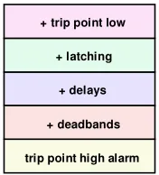
As the model has to handle sets of different states simultaneously, this is a potentially complex task. To minimise complexity, a layered implementation approach was adopted as shown in Figure 8.
Figure 8. Implementation of the non-deterministic machine + deadbands
+ delays + latching + trip point low
[image:7.612.262.350.604.701.2]A layered model of alarms is a clean solution, as it divides the problem of modelling the alarm into a set of simple, self-contained sub problems, each of which uses exclusively the model in the hierarchy located directly below itself.
At the bottom of the hierarchy there is a very simple model of an alarm with maximally reduced configuration options. Then a set of more sophisticated alarm models is built on top of that. All of them are, however, internally simple as each of them adds one configuration parameter only and reuses the functionality modelled by the alarm in the layer below.
The lowest layer state machine models a trip point high alarm with a configurable limit. This model is very simple as it only checks if the input value is in the uncertainty band. If so the model returns ‘UNCERTAIN’, otherwise it returns ‘ON’ or ‘OFF’ depending on whether the input is above or below the limit.
The next layer adds deadbands to the model. This is simple again as we can define two trip point high alarms: one with the same limit as the considered alarm, and the other with the limit set to (limit – deadband). We check what the outputs for a given input from both models are and based on this information we can easily infer the proper output for the model with the deadband.
The next layer adds delays. To create this model we use a model with deadbands, we store the previous alarm state, and the length of time the alarm was in the alarm state (a range from minimum to maximum). Using this information we infer the new state of the alarm.
Latching is similar. Again we need to remember the previous alarm state and based on this information and the state of the reset button we pass the value from the bottom layer or we set ‘ON’ as the output.
A similar layered model could have been constructed for the low trip function. But this was not necessary because a low trip can be simulated by applying a symmetrical transformation to the high trip model. Each input x is replaced by (RANGE – x), where RANGE is the maximum acceptable input value, and each decision point setting y is replaced by (RANGE – y).
For modelling the exact functionality of a smart instrument defined in section 2 we recommend layers defined as in Figure 8.
5.3. Selective (rule-based) verification
In contrast to the previous approaches, this result checking method is selective because it ignores test cases where the input sequence could result in a non deterministic output.
The basic idea is to specify a set of rules about the expected device behaviour. The rules are similar to the trace specifications used in temporal logic (e.g. Alur and Henzinger, 1994). Each rule specifies a sequence of inputs over time that meets certain constraints and the expected (deterministic) result if the sequence conditions are met. During the result checking, each rule is checked to see if the trace condition is true and if so, the expected result is checked. A discrepancy is reported if any of the applicable rules are violated. Each rule is a statement of the form:
{init:}input_traceexpected-response
Figure 9. Rule form
where:
− init is an optional initial device state (like configuration settings and device output states)
− input-trace is a sequence of constraints on the input value over some period of time.
− expected-response is a condition expressed in terms of one or more output values that should be true if the input trace condition is true.
Some example rules are shown in Figure 10.
Rule 1: [input >> limit] >> delay alarm=on
Rule 2: (input << limit) & reset alarm=off
Figure 10. Examples of rules of behaviour
the condition is true and the “>>” operator applied to the time-range tests that the range has definitely exceeded some limit (given known timing uncertainties).
Rule 2 states that whenever the input is below the limit and the reset button is pressed the alarm should be set off. This rule has no time-range, i.e. it is true for a particular test step. However there is an implicit time range which is the interval between test steps. A more formal definition of a rule is shown in Figure 11 below.
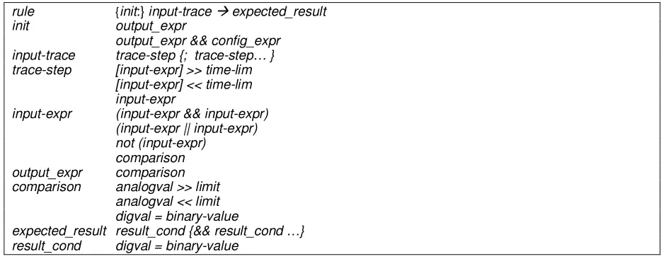
rule {init:} input-trace expected_result
init output_expr
output_expr && config_expr input-trace trace-step {; trace-step… } trace-step [input-expr] >> time-lim
[input-expr] << time-lim input-expr
input-expr (input-expr && input-expr) (input-expr || input-expr) not (input-expr) comparison output_expr comparison comparison analogval >> limit
analogval << limit digval = binary-value
[image:9.612.71.538.135.318.2]expected_result result_cond {&& result_cond …} result_cond digval = binary-value
Figure 11. The elements of a rule
Note that the construct {; trace-step… } indicates an optional sequence of additional terms of the same type. Additional entries on additional lines are alternative expansions of the left-hand term, and the expansion can be recursive if the term also appears on the right hand side. The “&&” and “||” terms denote the boolean AND and OR operations.
Ideally the rules should be expressed directly in this format and translated into a form suitable for checking. In practice, we implemented the rules directly as Perl functions that are still relatively easy to define and understand. For example Rule 1 in Figure 10 is actually expressed as:
whenever(above($hi_lim)); exceeds($timelim); expect( $hi_trip==1);
Figure 12. Perl implementation of Rule 1
The above function checks the analogue test value against a limit (taking account of measurement inaccuracy). The whenever function measures the time this condition is true over a series of test inputs, and exceeds checks whether this time exceeds the limit (taking account of timing inaccuracy). Finally expect checks the expected output state when the trace condition is satisfied.
The rule checker also requires parameters to be set that mirror the configuration of the actual device, and appropriate measurement and timing accuracy values have to be defined for use in the Perl checking functions (exceeds, above, below, etc).
5.4. Assessment of the options
Of the model-based approaches, we consider the non-deterministic state machine to be better than the parallel state machine method because:
− The modelling makes fewer assumptions about the internal design (like some possibly unknown input sampling interval) by permitting different interpretations of the input to occur at any point within a time range.
− The implementation is more efficient (fewer resources are needed).
effort is required to implement and validate the model. We quite often found that apparent discrepancies were actually due to some implied assumption in the model, which had to be removed.
By contrast the main advantages of the rule-based verification method are
− The behaviour description does not have to be complete. The rules can focus on the most important properties of the device.
− The rules are independent. So it is easy to add new rules and check if they are valid.
The main disadvantage is that the rule coverage is not necessarily complete, so some deterministic cases could be omitted. For example, if the input trace just touches the trip limit, Rule 1 in Figure 9 will not match because it does not “definitely exceed” the limit. A model-based checker would observe (for example) that the device had tripped on a particular input and update its internal model of the device state, so if the alarm subsequently cleared in the deadband, it would detect this as a discrepancy. The coverage of a rule-based checker can be increased by including an initial device output condition. For example, a rule that detects the device alarm has activated, can then detect an anomalous alarm clearance in the deadband. But typically a rule based checker is better-suited to situations where we are more interested in checking certain properties of device rather than thoroughly analysing all possible responses.
We recommend using the non-deterministic state machine in situations when we want to prove correctness of the whole data set.
We recommend using the rule-based verification in situations in which partial results are satisfactory, e.g. we want to be sure that the alarm will always be activated under specified conditions.
6. CASE STUDIES
In this section we present a case study that compares the application of model-based and rule-based checking to a smart device. Both types of checking were applied to two different programmable alarms (AL1 and AL2) which had nominally identical alarm functionality.
Both alarms were tested with a large number of test values (in excess of 100 000 tests at 2 second intervals) over a period of several days. This test sequence included many thousands of test cases that would trigger the high and low trip alarms in the device.
These test result files were analysed using both checkers. The non-deterministic state machine used the five layers described in section 5.2. The rule based checker had 6 rules defined for the high trip and an equivalent set of 6 rules for the low trip. Both checkers analysed all the test results in less than a minute.
The non-deterministic model checker reported no discrepancies for AL1 but a large number of discrepancies for AL2. By contrast, rule-based checking of exactly the same test result files reported no discrepancies in either programmable alarm.
Upon investigation we found there was a subtle difference in the functional behaviour of the two devices. With device AL1 the input trace has to be above the limit for the whole of the delay interval before the alarm activates, as shown in Figure 13 below.
Start Timer
Alarm Off Alarm On Delay interval
Limit
[image:10.612.89.522.525.660.2]Deadband
Figure 13. Alarm response of device AL1
Start Timer
Alarm Off Alarm
On Delay interval
Figure 14. Alarm response of device AL2
The non-deterministic model checker was originally developed to test device AL1, and used the interpretation of the alarm behaviour shown in Figure 13. As a result, when the checker was applied to AL2, discrepancies were generated when the AL2 alarm was activated earlier than expected.
By contrast, the rule-based checker had no rule for checking the early alarm scenario shown in Figure 14, but there were rules to check that the alarm was definitely off when below the deadband and definitely on when above the limit, so both devices satisfied these rules.
Once this difference in device behaviour was identified, it was easy to add an extra rule (activated by the observed output state of the alarm) to the rule-based checker that corresponded to the more “trigger happy” behaviour of device AL2. With this rule-set, no discrepancies were detected with device AL2, but discrepancies were reported for device AL1 as the new rule checks for alarm operation in the “trigger happy” region. This shows that a rule-based checker can differentiate between small variations in device behaviour given sufficient rules.
6. CONCLUSIONS
In this paper we presented a method of black-box testing of smart instruments. The test approach presented should be applicable to a wide range of smart devices. We made practical recommendations that summarise the important lessons learnt from the black box assessments we have performed. We believe that this paper is a good starting point for anybody wishing to perform a similar analysis of a computer-based system that makes decisions based on inputs that are subject to measurement uncertainty.
In the paper we focused particularly on the most difficult part of the black-box testing, which is the analysis of test results. Out of three different ways of building result checkers we recommended two, and their performance is compared in a case study.
Based on our current experience it is not obvious that any of the checking methods, i.e. the non deterministic state machine and the rule-based verification, is the best in all circumstances. The application context will determine which is the most suitable. For example, if there is an application requirement that the device must operate within some time constraint when some input limit is reached, then a rule-based check is the most appropriate. Such generic checks can be applied to diversely implemented devices and can tolerate minor differences in device behaviour. On the other hand, if we want to test for exact compliance of a device to its specification, a model-based checker is more appropriate.
In the next stage of the research we plan to apply our analysis to other smart instruments. This should help us better understand the suitability of alternative result checking methods. Further experience should also help to refine the recommendations we have made on the implementation of the test environment.
Acknowledgements
The authors wish to acknowledge the support of the UK Control and Instrumentation Nuclear Industry Forum (CINIF) who funded the research presented in this paper.
References
[1] Bishop, PG. Bloomfield, RE, Guerra, ASL and Tourlas, K, 2005. Justification of Smart Sensors for Nuclear Applications. In Winther, R., Gran, B.A., Dahll, G. (Eds.), SAFECOMP 2005. LNCS, vol. 3688, Springer, Heidelberg: 194–207.
[2] Alur, R. and Henzinger, T. 1994. A Really Temporal Logic. Journal of the ACM (JACM) 41(1): 181– 203.