City, University of London Institutional Repository
Citation
:
Bernardy, J. P., Jannson, P. and Paterson, R. A. (2012). Proofs for free -
parametricity for dependent types. Journal of Functional Programming, 22(2), pp. 107-152.
doi: 10.1017/S0956796812000056
This is the unspecified version of the paper.
This version of the publication may differ from the final published
version.
Permanent repository link: http://openaccess.city.ac.uk/1072/
Link to published version
:
http://dx.doi.org/10.1017/S0956796812000056
Copyright and reuse:
City Research Online aims to make research
outputs of City, University of London available to a wider audience.
Copyright and Moral Rights remain with the author(s) and/or copyright
holders. URLs from City Research Online may be freely distributed and
linked to.
doi:10.1017/S0956796812000056
Proofs for free
Parametricity for dependent types
J E A N-P H I L I P P E B E R N A R D Y and P A T R I K J A N S S O N Chalmers University of Technology & University of Gothenburg, Sweden
(e-mail:){bernardy,patrikj}@chalmers.se)
R O S S P A T E R S O N City University, London, UK
(e-mail:)[email protected])
Abstract
Reynolds’ abstraction theorem (Reynolds, J. C. (1983) Types, abstraction and parametric polymorphism,Inf. Process.83(1), 513–523) shows how a typing judgement in System F can be translated into a relational statement (in second-order predicate logic) about inhabitants of the type. We obtain a similar result for pure type systems (PTSs): for any PTS used as a programming language, there is a PTS that can be used as a logic for parametricity. Types in the source PTS are translated to relations (expressed as types) in the target. Similarly, values of a given type are translated to proofs that the values satisfy the relational interpretation. We extend the result to inductive families. We also show that the assumption that every term satisfies the parametricity condition generated by its type is consistent with the generated logic.
1 Introduction
Types are used in many parts of computer science to keep track of different kinds of values and to keep software from going wrong. Starting from the presentation of the simply typed lambda calculus by Church (1940), we have seen a steady flow of typed languages and calculi. With increasingly rich type systems came more refined properties about well-typed terms. In hisabstraction theorem, Reynolds (1983) defined a relational interpretation of System F types, and showed that interpretations of a well-typed term in related contexts yield related results. If a type has no free variables, the relational interpretation can thus be viewed as aparametricityproperty satisfied by all terms of that type. Almost 20 years ago Barendregt (1992) described a common framework for a large family of calculi with expressive types: Pure Type Systems (PTSs). By the Curry–Howard correspondence, the calculi in the PTS family can be seen both as programming languages and as logics. The more advanced calculi go beyond System F and include full-dependent types and support expressing datatypes.
results for several such calculi, but not in a common framework. In this paper, we apply and extend Reynolds’ (1983) idea to a large class of PTSs and provide a framework that unifies previous descriptions of parametricity and forms a basis for future studies of parametricity in specific type systems. As a by-product, we get parametricity for dependently typed languages. This paper is an extended and revised version of Bernardyet al. (2010). Our specific contributions are as follows:
• A concise definition of the translation of types to relations (Definition 3.9), which yields parametricity propositions for closed terms.
• A formulation (and a proof) of the abstraction theorem for PTSs (Theo-rem 3.12). A (Theo-remarkable feature of the theo(Theo-rem is that the translation from types to relations and the translation from terms to proofs are unified. • An extension of the PTS framework to capture explicit syntax (Section 4). • An extension of the translation to inductive definitions (Section 5), and its
proof of correctness.
• A formulation of an axiom schema able to internalise the abstraction theorem in a PTS. The axiom schema is proved consistent, thanks to a translation to PTS without axioms (Section 6).
• A specialisation of the general framework to constructs such as propositions, type classes, and constructor classes (Section 7).
• A demonstration by example of how to derive free theorems for (and as) dependently typed functions (Sections 3.3, 5, and 7).
Our examples use a notation close to that of Agda (Norell 2007), for greater familiarity for users of dependently typed functional programming languages. The notation takes advantage of the “implicit syntax” feature, improving the readability of examples.
2 Pure type systems
In this section we review the notion of PTS as described by Barendregt (1992, Sec. 5.2). We introduce our notation along the way, as well as our running example type systems.
Definition 2.1(Syntax of terms)
A PTS is a type system over aλ-calculus with the following syntax:
T=C constant
| V variable
| T T application
| λV:T.T abstraction
| ∀V:T. T dependent function space
c:s∈A
c:s
axiom
ΓA:s
Γ,x:Ax:A
start
ΓA:B ΓC:s
Γ,x:CA:B
weakening
ΓA:s1 Γ,x:AB:s2
(s1, s2, s3)∈R
Γ(∀x:A. B) :s3
product
ΓF: (∀x:A. B) Γa:A
ΓF a:B[x→a] application
Γ,x:Ab:B Γ(∀x:A. B) :s
Γ(λx:A. b) : (∀x:A. B) abstraction
ΓA:B ΓB:s B=βB
ΓA:B
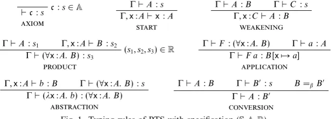
[image:4.493.71.410.61.183.2]conversion Fig. 1. Typing rules of PTS with specification (S,A,R).
The typing judgement of a PTS is parametrised over aspecification S= (S,A,R), where S ⊆C, A ⊆C×S, and R⊆S×S×S. The set S specifies the sorts, A the axioms (an axiom (c, s)∈A is often writtenc:s), andR specifies the typing rules of the function space. A rule (s1, s2, s2), where the second and third sorts coincide, is
often written s1;s2. The typing rules for a PTS are shown in Figure 1.
An attractive feature of PTSs is that the syntax for types and values is unified. It is the type of a term that tells how to interpret it (as a value, type, kind, etc.).
The λ-cube Barendregt (1992) defined a family of calculi each with S = {,}, A={:}andRa selection of rules of the forms1;s2, for example:
• The (monomorphic)λ-calculus hasRλ ={;}, corresponding to ordinary
(value-level, non-dependent) functions.
• System F hasRF=Rλ∪ {;}, adding (impredicative) universal
quantifi-cation over types (thus including functions from types to values). • System Fωhas RFω=RF∪ {;}, adding type-level functions.
• The Calculus of Constructions (CC) has RCC = RFω ∪ { ; }, adding
dependent types (functions from values to types).
Hereandare conventionally called the sorts oftypes andkinds, respectively. Notice that F is a subsystem of Fω, which is itself a subsystem of CC. (We say that S1 = (S1,A1,R1) is a subsystem of S2 = (S2,A2,R2) when S1 ⊆S2, A1 ⊆A2
and R1 ⊆R2.) In fact, the λ-cube is so named because the lattice of the subsystem
relation between all the systems forms a cube, with CC at the top.
Sort hierarchies Difficulties with impredicativity1 have led to the development of
type systems with an infinite hierarchy of sorts. The “pure” part of such a system can be captured in the following PTS, which we name Iω.
Definition 2.2 (Iω)
Iω is a PTS with this specification:
• S={i |i∈N}
• A={i:i+1 |i∈N}
• R={(i, j, max(i,j))|i, j ∈N}
Compared to the monomorphic λ-calculus, has been expanded into the infinite hierarchy0, 1, . . .InIω, the sort0 (abbreviated) is called the sort of types. Type
constructors, or type-level functions have type → . Terms like (representing the set of types) and → (representing the set of type constructors) have type 1
(the sort of kinds). Terms like1 and→ 1 have type2, and so on.
Although the infinite sort hierarchy was introduced to avoid impredicativity, they can in fact coexist, as Coquand (1986) has shown. For example, in the Generalised Calculus of Constructions (CCω) of Miquel (2001), impredicativity exists for the
sort (conventionally called the sort of propositions), which lies at the bottom of the hierarchy.
Definition 2.3(CCω)
CCω is a PTS with this specification:
• S={} ∪ {i |i∈N}
• A={:0} ∪ {i:i+1 |i∈N}
• R={;, ;i,i;|i∈N} ∪
{(i,j,max(i,j))|i, j∈N}
In the above definition, impredicativity is implemented by the rules of the form
i;.
Both CC andIω are subsystems of CCω, with i in Iω corresponding to i in
CCω. Becausein CC corresponds to0 in CCω, we often abbreviate0 to.
Many dependently typed programming languages and proof assistants are based on variants ofIω or CCω, often with the addition of inductive definitions
(Paulin-Mohring 1993; Dybjer 1994). Such tools include Agda (Norell 2007), Coq (The Coq development team 2010) and Epigram (McBride & McKinna 2004).
2.1 Pure type system as logical framework
Another use for PTSs is as logical frameworks: types correspond to propositions and terms to proofs. This correspondence extends to all aspects of the systems and is widely known as the Curry–Howard isomorphism. The judgementp:P means thatp is awitness, orproof of the propositionP. If the judgement holds (for some p), we say thatP isinhabited.
In the logical system reading, an inhabited type corresponds to a tautology and dependent function types correspond to universal quantification. A predicateP over a type A has the type A → s, for some sort s: a value a satisfies the predicate whenever the type P a is inhabited. Similarly, binary relations between values of typesA1 andA2 have typeA1→A2→s.
For this approach to be safe, it is important that the system beconsistent. In fact, the particular systems used here even exhibit the strong normalisation property: each witnessp reduces to a normal form.
In fact, inIω and similarly rich type systems, one may represent both programs
this property: We encode programs and parametricity statements about them in the same type system.
3 The relational interpretation
In this section we present the core contribution of this paper: The relational interpretation of a term, as a syntactic translation from terms representing programs or types (in a source PTS understood as a programming language) to terms representing proofs or relations (in a target PTS understood as a logic expressing properties of programming language terms). As we will see in Section 3.3, it is a generalisation of the classical rules given by Reynolds (1983), extended to all the constructs found in a PTS.
3.1 Preliminaries
Usual presentations of parametricity use binary relations, but for generality we abstract over the arity of relations,n, which we assume is given. We use an overbar notation to denote parts of terms being replicated n times with renaming, defined formally as follows.
Definition 3.1 (renaming)
The termAiis obtained by replacing each free variablexin the termAby a variable
xi.
Definition 3.2 (replication)
A stands forn terms Ai, each obtained by renaming as defined above.
Correspond-ingly,x:Astands fornbindings (xi:Ai). If replication is used in a binder (abstraction
or dependent function space), then the binder is also replicated.
For a particular source PTS S, we shall require a target PTS Sr that includes S
so that source terms can be expressed, but also sufficient sorts, axioms and rules to express the relational counterparts of the source terms. For example, we require that for each sortsinS,Sr should also include a sortsthat will be the sort of relational propositions about terms of sort s. In many cases we uses=s.
Below we simply list our requirements on Sr, noting where we shall need them
later. The need for each of these requirements should become clear when we reach those points in our development. For a first approximation, we assume that the only constants in S are sorts. We return to the general case in Section 5.
Definition 3.3 (reflecting system)
A PTSSr= (Sr,Ar,Rr)reflects a PTSS= (S,A,R) ifS is a subsystem ofSr and
1. (needed for Lemma 3.7) for each sorts∈S, • Sr contains sortss,s,sands
• Ar contains s:s,s:s ands:s • Rr contains s;s ands;s
3. (needed for the translation of products) for each rule (s1, s2, s3)∈R,Rrcontains
rules (s1,s2,s3) ands1;s3.
Example 3.4
The system CCωreflects each of the systems in theλ-cube, withs=s.
Definition 3.5(reflective)
We say thatS is reflective ifS reflects itself withs=s. Example 3.6
The systems Iω and CCω are both reflective. Therefore, we can write programs in
these systems and derive valid statements about them, within the same PTS.
3.2 From types to relations, from terms to proofs
In this section we present the relational translation of terms. We discuss the intuition behind each case of the definition before summarising them (in Definition 3.9).
The translation of a sort s forms types of n-ary relations between types of sort s. In particular, we choose to model relations between types A1, . . . , An of sort sas
terms of typeA1→ · · · →An→s, wheresis the sort of propositions corresponding
to types of sorts. (In many cases we uses=s.) Thus, we define the translation ofsas
s=λx:s.x→s
Then lambda-abstractions over the variablesxname the parameter types of sort s, from which the type of relations is formed.
Lemma 3.7(sis well-typed)
If the PTSSrreflects the PTSS, then for each sorts∈Swe haves:s→sinSr.
Proof
From the requirements for a sort s∈ S in the first part of Definition 3.3, we can infer (inSr)
s:s st
x:sxi:s
s:s s:s wk
x:ss:s s;s
x:sx→s:s
s:s s:s
s;s s→s:s
abs
(λx:s.x→s) :s→s
Moreover, if two sorts are related by an axiom, their translations are related. Lemma 3.8
If the PTSSr reflects the PTSSandAcontains an axioms:t, thens:t sinSr.
Proof
..
. Lemma 3.7 s:s→s
..
. Lemma 3.7
(λx:t.x→t) :t→t s:t app (λx:t.x→t)s:t
conv,s=t
s: (λx:t.x→t)s
Generalising Lemma 3.8, for each type A : s, we wish to define a relation
A:sA. Type systems usually include constants that are not sorts, but as their meaning is unconstrained, we cannot expect a generic translation for them. We shall deal with such constants in Section 5.
We shall approach dependent product types through special cases. Firstly, the relation A → B relates functions if they map inputs related by A to outputs related byB:
A→B=λf: (A→B).∀x:A.Ax→B(f x)
Secondly, the relation ∀x:s. B relates polymorphic terms if their instances at related types are related:
∀x:s. B=λf: (∀x:s. B).∀x:s.∀xR:x→s.B(f x)
=λf: (∀x:s. B).∀x:s.∀xR:sx.B(f x)
Both of these forms are special cases of the general translation of products as follows:
∀x:A. B=λf: (∀x:A. B).∀x:A.∀xR:Ax. B(f x)
Products are also types, and hence are also translated to relations via lambda-abstractions over n functions f. The right-hand side of the product ends the description of how the functions f must be related by requiring that the result of applying f toxbe related by the translation of B.
In the above translation, if the source product ∀x:A. B is formed with the rule (s1, s2, s3), then Ax has sort s1, while B(f x) has sort s2. Thus, Sr requires the
rule (s1,s2,s3) in order to form the inner product on the right-hand side. Similarly,
the outer product requires the rules1 ;s3. These rules are those of the third part
of Definition 3.3.
The translation of applications and abstraction mirrors the translation of product types at the value level: one argument is mapped to n arguments and a relation argument,
F a=Faa
λx:A. b=λx:A. λxR:Ax. b
The translation maintains the invariant that for each free variable in the inputx, the output hasn+ 1 free variables, x1, . . . ,xn and xR, wherexR witnesses that x1, . . . ,xn
are related. Hence, a variablexcan be translated toxR.
The translation of terms is summed up in the following definition, which gives the mapping from terms of a PTS S to terms of a possibly extended PTS Sr as
Definition 3.9(parametricity translation from types to relations)
s=λx:s.x→s
x=xR
∀x:A. B=λf: (∀x:A. B).∀x:A.∀xR:Ax.B(f x) F a=Faa
λx:A. b=λx:A. λxR:Ax.b
The replication of variables carries on to contexts.
Definition 3.10(parametricity translation for contexts)
–= –
Γ, x:A=Γ, x:A, xR:Ax
Note that each tuplex:A in the translated context must satisfy the relationA, as witnessed byxR. Thus, one may interpret Γ asn related environments; and Aas
ninterpretations ofA, each one in a different environment.
Lemma 3.11(translation preserves β-reduction)
A−→∗βA =⇒ A−→∗β A Proof sketch
The proof proceeds by induction on the derivation of A −→∗β A. The interesting case is where the termA is a β-redex (λx:B. C)b. That case relies on the way interacts with substitution:
b[x→C]=b[x→C][xR→C]
The remaining cases are congruences.
We can then state our main result.
Theorem 3.12(abstraction) If the PTSSr reflects the PTS S,
ΓS A:B =⇒ ΓSr A:BA
Proof
By induction on the derivation of ΓS A:B. Each typing rule in the derivation
of the source judgement can be translated to a portion of the derivation tree of the target. The start case is a consequence of the invariant that a relational
witness is always introduced in the context when a variable is bound in the source term. The cases of abstraction and application stem from the fact that their
productcase uses the fact that types are translated to relations (ins), and imposes
constraints on the structure of the target PTS (see Definition 3.3). In theaxiomcase,
we rely on the “types-to-relations” principle at two different levels, and further conditions are imposed on the target PTS. More details of the proof are given in
Appendix A.1.
The above theorem can be read in two ways. A direct reading is as a typing judgement about translated terms: if A has typeB, then A has typeBA. The more fruitful reading is as an abstraction theorem for PTSs: if A has type B in environment Γ, thenn interpretationsAin related environments Γare related by
B. Further,Ais a witness of this propositionwithin the type system. In particular, closed terms are related to themselves:A:B =⇒ A:BA . . . A.
3.3 Examples: the λ-cube
In this section we show that specialises to the rules given by Reynolds (1983) to read a System F type as a relation. Having shown that our framework can explain parametricity theorems for System F types, we move on to progressively higher order constructs. In these examples, the binary version of parametricity is used (arity n= 2). Using Definition 3.3 one can verify that the following system reflects System F.
• S={,,1,, ,1,2}
• A={:,:1,:, :1,1:2}
• R={;,;, ;,;1,1;2,;, ;}
Indeed, examination of the structure of the PTS reveals that it corresponds to a second-order logic with typed individuals, studied multiple times in the literature with slight variations, for example by Plotkin & Abadi (1993) or Wadler (2007). In the PTS form, the sort is the sort of propositions. The sort is inhabited by the type of propositions (), the type of predicates (τ→), and in general types of relations (τ1 → · · · → τn → ). The sorts1 and 2 come from the need to type
unimportant higher level redexes created by our translation, and correspond to the sorts with the same name in CCω. The product formation rules can be understood
as follows:
• ;allows to build implication between propositions; • ;allows to quantify over programs in propositions; • ;allows to quantify over types in propositions;
• ; is used to build types of predicates depending on programs; • ;allows to quantify over predicates in propositions.
• The other rules, involving1and2 come from the need to type higher level
relation-membership redexes.
Types to relations Note that by definition,
T1T2 = T1 → T2 →
Function types Applying our translation to a closed non-dependent function type, we get:
A → B :(A → B) (A → B)
A → Bf1f2 = ∀a1 :A. ∀a2 : A. Aa1a2 → B(f1a1) (f2a2)
That is, functions are related iff they take related arguments into related outputs.
Type schemes System F includes universal quantification of the form ∀A:. B. Applying to this type expression yields:
∀A :. B :(∀A: . B) (∀A : . B)
∀A :. Bg1g2 = ∀A1 : . ∀A2 : . ∀AR :A1A2. B(g1 A1) (g2A2)
In words, polymorphic values are related iff instances at related types are related. Note that becauseA may occur free in B, the variables A1, A2, andAR may occur
free inB.
Type constructors With the addition of the rule ; , one can construct terms of type → , which are sometimes known as type constructors, type formers, or type-level functions. As Voigtl¨ander (2009) remarks, extending the Reynolds-style parametricity to support-type constructors appears to be a folklore. Such folklore can be precisely justified by our framework by applying to obtain the relational counterpart of type constructors:
→ :( → ) (→ )
→ F1F2 = ∀A1 : . ∀A2 : . A1A2 →(F1A1) (F2A2)
That is, a term of type → F1 F2 is a (polymorphic) function converting a
relation between any types A1 and A2 to a relation between F1 A1 and F2 A2, a
relational action. For the target system to accept the above, the rules ; and
; must also be added there.
Dependent functions In a system with the rule;, value variables may occur in dependent function types like∀x:A. B, which we translate as follows:
∀x :A. B : (∀x : A. B) (∀x :A. B)
∀x :A. Bf1 f2 = ∀x1 : A. ∀x2 : A. ∀xR : Ax1x2. B(f1x1) (f2x2)
Proof terms We have used to turn types into relations, but we can also use it to turn terms into proofs of abstraction properties. As a simple example, the relation corresponding to the typeT = (A :) → A→A, namely
Tf1f2 = ∀A1 : . ∀A2 : . ∀AR :A1A2.
∀x1 : A1. ∀x2 : A2. ARx1 x2→AR(f1A1x1) (f2A2x2)
states that functions of typeTmap related inputs to related outputs, for any relation. From a term id = λA : ∗. λx : A.x of this type, by the abstraction theorem we obtain a termid: Tid id, that is a proof of the abstraction property:
idA1A2ARx1x2xR = xR
We return to proof terms in Section 5.3 after introducing datatypes.
4 Coloured pure type systems
In this section we introduce the notion of coloured pure type system (CPTS), which is an extension of PTS as described in Section 2. Colours capture the fact that various flavours of quantification use different syntax. We use colours to improve the clarity of the relational translation as well as that of examples.
4.1 Explicit Syntax: Coloured Pure Type Systems
The complete uniformity of syntax characteristic of classical presentations of the PTS framework often obscures the structure of ideas expressed within particular PTS, and our relational interpretation of terms in no exception. While mere PTSs are sufficient for most of the technical results of this paper, the structure of the relational interpretation appears more clearly when various flavours of quantification are properly identified.
Explicit syntax in PTSs is not novel: Many systems usually presented as PTSs still use different syntax for various forms of quantifications. For example, traditional presentations of System F use a different syntax for the quantification over individ-uals (rule ;) than for the quantification over types (rule ;). A common practice is to use the symbols∀and Λ for quantification and abstraction over types, and → and λ for individuals. In addition, brackets are sometimes used to mark type application. While the flavour of quantification can always be recovered from a type derivation, the advantage of explicit syntax is that it is possible to identify which flavour is used merely by looking at the term. Moreover, a type-derivation tree might not be available.
In this paper we want to give a relational interpretation of terms parameterised over any PTS, and retain the possibility to keep syntax annotations. This is exactly the purpose of CPTSs: to capture explicit syntax in a parametrised way. A colour annotation is added to the syntax of application, abstraction, and product, and a colour component is added to R. A rule (k, s1, s2, s2) is often written s1
k
;s2. Note
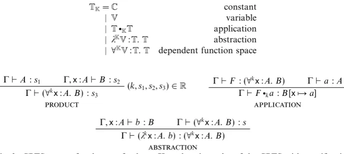
TK=C constant
| V variable
| T•KT application
| λKV:T.T abstraction | ∀KV:T.T dependent function space
ΓA:s1 Γ,x:AB:s2
(k, s1, s2, s3)∈R
Γ(∀kx:A. B) :s
3
product
ΓF: (∀kx:A. B) Γa:A ΓF•ka:B[x→a]
application
Γ,x:Ab:B Γ(∀kx:A. B) :s Γ(λkx:A. b) : (∀kx:A. B)
[image:13.493.81.426.60.215.2]abstraction
Fig. 2. CPTS syntax for the set of coloursK, and typing rules of the CPTS with specification (K,S,A,R). The only change with respect to the standard PTS definition is the addition of colour annotations in product, application, and abstraction.
ensure that the colours are matched (Figure 2). Erasure of colour yields a plain (monochrome) PTS; and erasure of colour in a valid coloured derivation tree yields a valid derivation tree in the monochrome PTS. Therefore, useful properties of PTSs (such as subject reduction, substitution, etc.) are retained in CPTSs.
4.2 Relational translation, with colour
We can modify our translation to use colours to distinguish the two kinds of arguments it introduces so that a single product of colour k is translated to two kinds of products,n of colourki, which introducesn termsxof type Ai, and one of
colourkr, which forces them (x) to be related by the translation ofA. (Memory aid:
istands for individual andrfor relation.)
∀kx:A. B=λf: (∀kx:A. B). ∀kix:A.∀krx
R:Ax.B(f•kx)
F•ka=F•kia•kra
λkx:A. b=λkix:A. λkrx
R:Ax.b
We use a special, new colour (named 0 below) for the formation of relations that interpret types. Since this colour is used very many times, leave out the annotation for it. Using this convention, the translation of a sortslooks exactly the same when colours are used as in the monochrome case:
s=λx:s.x→s
The colour 0 was already used in the first set of equations given in this section, for example, in the abstraction over f, or in the applications of A. Thanks to colours, it becomes syntactically obvious that the abstraction over f creates a relation (interpreting a type), whereas the abstraction overx does not.
Definition 4.1 (reflecting system, with colour)
A CPTSSr = (Kr,Sr,Ar,Rr)reflects a CPTSS = (K,S,A,R) ifS is a subsystem of
Sr and
1. there is a colour 0∈Kr, used for relation construction. Annotations for this
colour are consistently omitted in the remainder of the section, 2. there are two functions iand r fromKtoKr,
3. for each sorts∈S,
• Sr contains sortss,s,sands • Ar contains s:s,s:s ands:s
• Rr contains s;s ands;s
4. for each axioms:t∈A,s=t,
5. for each rule (k, s1, s2, s3)∈R, Rr contains rules (kr,s1,s2,s3) ands1
ki
;s3.
Remark 4.2
The above definition is intuitively justified as follows:
1. The colour 0 is used for formation of parametricity relations. 2. For each colourk∈K,
• the colour kiis used for universal quantification over individuals in logical
formulas;
• the colour kr is used for quantifications over propositions in the target
system.
3. For each sorts, the sortsis the sort of parametricity propositions about types ins, and must exist inSr. One can seeas a function fromStoSr.
For each input sort, the relational interpretation creates redexes, which check relation membership. This requires
• each input sort sto be typeable (i.e. inhabit another sort s– in the above definition we consistently use s for a sort thatsinhabits);
• two extra sorts in the target system (s,s) on top ofs; • rules to allow for the formation of relations.
4. The following two relations between sorts must commute: • axiomatic inhabitation (A);
• correspondence between a sort of types and a sort of relational propositions ().
This point is not a strict requirement for the abstraction theorem to hold. However, we found that without this requirement, the structure of the target system is too unconstrained to make intuitive sense of it.
5. For each type-formation rule of the input system, there is • a formation rule for quantification over individuals;
4.3 Coloured examples
A colour for naive set-theory Earlier in this paper, we have outlined how PTSs can be used to represent concepts like propositions and proofs. One may want to use special syntax for PTS constructs when the propositions-as-types interpretation is intended: even though propositions and types are syntactically unified in PTSs, it can be useful to make the intent explicit. Therefore, a special colour might be reserved for the purpose of expressing logical formulae in some CPTSs. A possible choice of concrete syntax is the following, reminiscent of naive set theory.
Tlogic=. . .
| T∈T (reverse application) | {V:T|T} (abstraction) | ∀V:T.T (quantification)
Classic presentations of parametricity use similar syntax, and by simply choosing this syntax for some of the colours in our PTSs, we are able to underline the similarity of our framework with previous work (Section 3.3).
A colour for implicit syntax Many proof assistants and dependently typed pro-gramming languages (including Agda, Coq, and LEGO) provide the so-called “implicit” syntax. The rationale for the feature is that, in the presence of precise type information, some parts of terms (applications or abstractions) can be fully inferred by the type-checker. In such cases, the user might want to actually leave out such parts of the terms. It is convenient to do so by marking certain quantifications as “implicit”. Then the presence of the corresponding applications and abstractions can be inferred by the type-checker.
Such marking can be modelled by a two-colour PTS: one colour for regular syntax, and another for “implicit syntax”. (Typically, every rule is available in both the colours.) The syntax of CPTSs does not allow for omission of terms though, so it can be used only for terms whose omitted parts have been filled in by the type-checker. Miquel (2001, section 1.3.2) gives a detailed overview of two-colour PTSs used for implicit syntax.
4.4 Implicit syntax
In the following sections, our examples are written using the Agda syntax, and take advantage of the implicit syntax feature. The following colour-set is used:K={e, i} (e= explicit colour;i= implicit colour). Rather than using colour annotations, the following (Agda-style) concrete syntax is used.
Definition 4.3(Agda-style syntax for two-colour PTS)
T=C constant
| V variable
| T T application
| λV:T. T abstraction
|T{T} implicit application |λ{V:T}.T implicit abstraction | {V:T} →T implicit dependent function space
In addition, implicit abstraction and application may be left out when the context allows it (we do not formalise this notion). We use the following colour-mappings:
0→e
ir→e ii→i
er→e ei→i
The instantiation of (Definition 3.9) to the above mapping yields the following translation if written with the Agda-style syntax.
Example 4.4 (translation from types to relations, specialised to implicit arguments)
s=λx:s.x→s
x=xR
(x:A)→B=λf: ((x:A)→B).{x:A} →(xR:Ax)→B(f x) F a=F{a}a
λx:A. b=λ{x:A}. λxR:Ax. b
{x:A} →B=λf: ({x:A} →B).{x:A} →(xR:Ax)→B(f{x}) F{a}=F{a}a
λ{x:A}. b=λ{x:A}. λxR:Ax. b
The usage of implicit syntax in the translation is not innocent: It is carefully designed to take advantage of the type-inference mechanism to allow shorter expressions of translations. For example, id, generated from id : T can now hide four out of six abstractions:
idARxR = xR
This example is typical. Indeed, we observed that for all termsAof typeB, given the typing constraintA:BA, arguments can be inferred at every implicit application in the expansion ofA. Likewise, every implicit abstraction is inferable and can be omitted. We have found these shortcuts to be essential to readability, as they hide much of the noise generated by the relational transformation. Therefore, we have taken advantage of inference wherever possible in the examples presented in this paper, starting from Section 5.
5 Constants and datatypes
constant andAan arbitrary term, not a mere sort) we require a termcsuch that the judgementSr c:Acholds. If the constants come with additional β-conversion
rules, the translation must also preserve conversion so that Lemma 3.11 holds in the extended system: for any termA involvingc, A−→βA =⇒ A−→∗βA.
One source of constants in many languages is datatype definitions. In the rest of this section we investigate the implications of parametricity conditions on datatypes, and give two translation schemes for inductive families (as an extension ofIω). In
Section 5.3 we show how the termccan be constructed from pairs and units, while in Section 5.4 we define it using another datatype definition (in which we have a constructor namedc).
5.1 Parametricity and elimination
Reynolds (1983) and Wadler (1989) assume that each type constant K : is translated to the identity relation. This definition is certainly compatible with the condition required by Theorem 3.12 for such constants:K : K K, but so are many other relations. Are we missing some restriction for constants? This question might be answered by resorting to a translation to pure terms via Church encodings (B¨ohm & Berarducci 1985) as Wadler (2007) does. However, in the hope to shed a different light on the issue, we give another explanation, using our machinery.
Consider a base type, such asBool : , equipped with constructorstrue : Bool
andfalse : Bool. In order to derive parametricity theorems in a system containing such a constant Bool, we must define Bool, satisfying Bool : Bool. What are the restrictions put on the termBool? First, we must be able to define
true : Booltrue. Therefore,Booltrue must be inhabited. The same reasoning holds for thefalsecase.
Second, to write any useful program using Booleans, a way to test their value is needed. This may be done by adding a constant
if : Bool→ (A : ) → A →A → A
such thatif true A x y −→β xandif false A x y −→β y.
Now, if a program usesif, we must also defineifof type
Bool→ (A : ) → A →A → Aif
for parametricity to work. Let us expand the type of if and attempt to give a definition case by case:
if : {b1b2 : Bool} → (bR :Boolb1b2)→
{A1A2 :} → (AR : A1A2) →
{x1 : A1} → {x2 : A2} → (xR : ARx1x2) →
{y1 : A1} → {y2 : A2} → (yR : ARy1y2) →
AR(if b1 A1 x1y1) (if b2 A2x2y2)
if{false} {true} bR xRyR = ?ft
if{false} {false}bR xRyR = yR
(From this example onwards, we use a layout convention to ease the reading of translated types: each triple of arguments, corresponding to one argument in the original function, is written on its own line if space permits.)
In order to complete the above definition, we must provide a type-correct term for each question mark. For ?tf, this means that we must construct a term of type
ARx1y2. NeitherxR : ARx1x2 noryR : ARy1y2 can help us here. The only liberty
left is in bR : Booltrue false. If we letBooltrue falsebe falsity (⊥, the empty
type), then this case can never be reached and we need not give an equation for it. This reasoning holds symmetrically for ?ft. Therefore, we have the restrictions:
Boolx x = some inhabited type
Boolx y = ⊥ ifx=y
We have some freedom regarding picking “some inhabited type”, so we choose
Boolx xto be truth (), makingBoolan encoding of the identity relation. An intuition behind parametricity is that, when programs “know” more about a type, the parametricity condition becomes stronger. The above example illustrates how this intuition can be captured within our framework: having the eliminator if
constrains the interpretation ofBool. We will make further use of this in Section 7.2.
5.2 Inductive families
Many languages permit datatype declarations for Bool,Nat,List, etc. Dependently typed languages typically allow the return types of constructors to have different arguments, yielding inductive families (Paulin-Mohring 1993; Dybjer 1994) such as the familyVec, in which the type is indexed by the number of elements. In Figure 3 we introduce Agdadatasyntax and some example datatypes and inductive families, which will be used later, including the sigma type, Σ which contains (dependent) pairs and the identity relation ≡ which contains proofs of reflexivity. We sometimes write (x:A)×B for Σ A (λx:A. B), and elements of this type as (a, b), omitting the arguments A andλx:A. B, handled by implicit syntax. For any valuesx and y
of type A, the term x≡y is a type, but only the types on the diagonal x≡x are inhabited (by the canonical termrefl).
In an “impure” PTS setting, datatype declarations can be interpreted as a simultaneous declaration of formation and introduction constants and also an eliminator and rules to analyse values of that datatype.
Example 5.1
The definition ofListin Figure 3 gives rise to the following constants and rules:
List : (A :) →
nil : {A: } → List A
data⊥: where -- no constructors data: where
tt:
dataBool :where false: Bool true : Bool dataNat: where
zero: Nat succ: Nat→ Nat
dataList(A: ) :where nil :List A
cons :A→ List A→ List A dataVec(A: ) :Nat→ where
nilV :Vec A zero
consV :A→ (n: Nat) → Vec A n→ Vec A(succ n) dataΣ(A: ) (B: A→ ) :where
, : (a :A) → B a→ Σ A B data ≡ {A: }(a : A) :A→ where
refl :a≡a
Fig. 3. Examples of simple datatypes and inductive families (introducing Agda datatype syntax through well-known examples).
List-elim: {A : } → (P: List A → )→ (base : P nil) →
(step : (x : A) →(xs : List A)→ P xs → P(cons x xs))→ (ys : List A)→ P ys
List-elim P base step nil = base
List-elim P base step(cons x xs) = step x xs(List-elim P base step xs) Note that the datatype parameterAis an implicit parameter of the constructor and eliminator constants.
More generally, family declarations of sorts(in the examples) have the typical form:2
dataT(a:A) : (n:N)→swhere
c: (b:B)→(u: ((x:X)→Tai))→Tav
Arguments of the type constructorTmay be either parametersa, which scope over the constructors and are repeated at each recursive use ofT, or indicesn, which may vary between uses. Data constructorschave non-recursive argumentsb, whose types are otherwise unrestricted, and recursive arguments u with types of a constrained form (Tcan not appear inX).
In PTS style we have the following formation and introduction constants:
T: (a:A)→(n:N)→s -- type
c :{a:A} →(b:B)→((x:X)→Tai)→Tav -- constructor and also a corresponding eliminator:
T-elim:{a:A} →
(P: ((n:N)→Ta n→s))→
Casec→(n:N)→(t:Ta n)→P n t
where the typeCasec of the case for each constructorcis
(b:B)→(u: ((x:X)→Tai))→((x:X)→Pi(u x))→Pv(c{a}b u)
2 We show only one of the each element (parametera, indexn, constructorc, etc.) here. The generalisation
with one evaluation rule (β-reduction) for each constructor c:
T-elim{a}P ev(c{a}b u) =e b u(λx:X.T-elim{a}P ei(u x)) (1)
As in the List example, the datatype parameter A is an implicit parameter of the constructor and eliminator constants.
We often use corresponding pattern matching definitions instead of these elimi-nators (Coquand 1992).
In the following sections, we consider two ways to “generically” define a proof termc:Tc. . .cfor each constantc:T introduced by the data definition.
5.3 Deductive-style translation
In Section 5.1 we gave a definition of Booland iffor a simplified eliminator if. In this subsection we present similar deductive-style translations for several concrete examples, and then deal with the general case. We define each proof as a term (using pattern matching to simplify the presentation) built up from simpler building blocks (pairs and units). (In Section 5.4 the inductive-style translation, we instead translate datatypes to families; datatodata.)
Lists From the definition of List in Figure 3, we have the constant List : → , so List is an example of a type constructor, and thus List should be a relation transformer. As withBool, lists are related only if their constructors match. Two
nillists are trivially related; as in theBoolcase we usefor the nullary constructor. Two cons lists are related only if their components are related; the proof of that relationship is a pair of proofs for the components, represented as a product (×):
List: → List List
ListARnil nil =
ListAR(cons x1xs1) (cons x2xs2) = ARx1x2 × ListARxs1xs2
ListAR = ⊥
This is exactly the definition of Wadler (1989): Lists are related iff their lengths are equal and their elements are related point-wise. The translations of the constructors build the corresponding proofs:
nil : (A: ) → List Anil nil
nilAR = tt
cons :(A : ) →A → List A →List Acons cons
consARxRxsR = (xR,xsR)
Applying the translation toRyields:
R : R→ R →
Rr1r2 = {A1A2 :} → (AR : A1A2) →
{xs1 : List A1} → {xs2 : List A2} → (xsR : ListARxs1xs2) →
ListAR(r1A1xs1) (r2 A2xs2)
In words: Two list rearrangementsr1 and r2 are related iff for all types A1 and A2
with relationAR, and for all listsxs1 andxs2 point-wise related byAR, the resulting
listsr1 A1 xs1 and r2 A2 xs2 are also point-wise related by AR. By Theorem 3.12, Rr rholds for any termrof typeR. This means that applyingrpreserves (point-wise) any relation existing between input lists of equal length. By specialisingAR to
a function (ARa1a2 = f a1≡a2), we obtain the following well-known result:
(A1A2 : ) → (f : A1 → A2) → (xs: List A1) →
map f(r A1xs)≡r A2(map f xs)
(This form relies on the facts that List preserves identities and composes with
map.)
Proof terms We have seen that applying to a type yields a parametricity property for terms of that type, and by Theorem 3.12 we can also apply to a term of that type to obtain a proof of the property. As an example, consider a rearrangement functionoddsthat returns every second element from a list:
odds : (A: ) → List A→ List A odds A nil = nil odds A(cons x nil) = cons x nil
odds A(cons x(cons xs)) = cons x(odds A xs)
Any list rearrangement function must satisfy the parametricity condition Rseen above, andoddsis a proof thatoddssatisfies parametricity. Expanding it yields:
odds : (A: ) → List A→ List Aodds odds
oddsAR{nil} {nil} = tt
oddsAR{cons x1nil} {cons x2nil}(xR, ) = (xR,tt)
oddsAR{cons x1(cons xs1)} {cons x2(cons xs2)}(xR,( ,xsR)) =
(xR,oddsAR{xs1} {xs2}xsR)
We see (by textual matching of the definitions) thatoddsperforms essentially the same computation as odds, on two lists in parallel. However, instead of building a new list, it keeps track of the relations (in the R-subscripted variables). This behaviour stems from the last two cases in the definition ofodds. Performing such a computation is enough to prove the parametricity condition.
Vectors The translations of the constants ofVecare simple extensions of those for
List, with an additional requirement that sizes be related by the identity relation
Vec : (A : ) → Nat → Vec
VecARnRnilV nilV =
VecAR{succ n1} {succ n2}nR(consV n1 x1xs1) (consV n2x2xs2) =
ARx1x2×(nR : Natn1n2)×VecARnR VecARnRxs1 xs2 = ⊥
nilV : {A: } → Vec A zeronilV
nilVAR = tt
consV: {A : } → A→ (n : Nat) → Vec A n → Vec A(succ n)consV
consVARxRnRxsR = (xR,(nR,xsR))
In the List example above we omitted the translation of the elimination constant
List-elim. Here we shall handle the more complexVec-elim, which has the type
Vec-elim : {A: } →
(P : (n :Nat) →Vec n A → ) → (en : P zero(nilV A)) →
(ec: (x : A) → (n :Nat) →(xs : Vec n A) →
P n xs → P(succ n) (consV x n xs))→ (n : Nat) → (v : Vec n A) → P n v
The translation of this constant has a large type, but a simple definition:
Vec-elim : {A :} →
(P : (n : Nat) →Vec n A →) → (en : P zero(nilV A))→
(ec: (x : A) → (n : Nat) → (xs: Vec n A) →
P n xs → P(succ n) (consV x n xs)) → (n : Nat) → (v : Vec n A) → P n vVec-elim
Vec-elimAR PRenRecR {nilV} {nilV} = enR
Vec-elimAR PRenRecRnR{consV x1n1 xs1} {consV x2n2xs2}(xR,(nR,xsR))
= ecRxRnRxsR(Vec-elimARPRenRecRnRxsR)
Dependent pairs Two pairs (a1,b1) and (a2,b2) are related by A×B if their
respective components are related (by Aand B). A constructive reading is that a proof that two pairs are related can be represented as a pair of proofs. This generalises nicely to the dependent case: a dependent pair (of the Σ type from Figure 3) translates to another dependent pair. That is, a pair (a,b) :Σ A B(where
a : Aandb : B a) translates to
(a,b) : Σ A B(a1,b1) (a2,b2)
where
Σ : {A1A2 :}(AR :A1 A2)
{B1 :A1 → } {B2 : A2 →}
(BR : {a1 : A1} {a2 :A2} → ARa1a2 → (B1a1) (B2a2)) →
(Σ A1B1) (Σ A2B2)
Inductive families – general case For the “typical form” of an inductive family we begin with the translation of Equation (1) for each constructorc:
T-elim{a}P ev(c{a}b u) (c{a}aR{b}bR{u}uR) =RHS (2)
for RHS = e b u (λx:X.T-elim {a} P e i (u x)). To turn this into a pattern matching definition of T-elim, we need a suitable definition ofc, and similarly for the constructors inv. The only arguments ofcnot already in scope arebR and
uR, so we package them as a dependent pair because the type ofuRmay depend on
that ofbR. We define
T:(a:A)→(n:N)→sT
T{a}aR{v}v(c{a}b u) = (bR:Bb)×(x:X)→Taiu T{a}aR{u}uRt =⊥
c:({a:A})→(b:B)→((x:X)→Tai)→Tavc
caRbRuR= (bR,uR)
Substituting the above definition ofcinto Equation (2), we obtain a clause for the definition ofT-elim:
T-elim{a}P ev(c{a}b u) (bR,uR) =RHS
These clauses cover only cases where the constructors match, but becauseTyields ⊥otherwise, that is complete coverage.
The question whether the translation of the eliminator and its reduction rule are inductively well-founded is delayed until we have completed the presentation of the Inductive-style translation.
5.4 Inductive-style translation
Another way of defining the translations c of the constants associated with a datatype is to use aninductive definition (usingdata) in contrast with thedeductive definitions (construction using pairs and units) of the previous section.
Deductive- and inductive-style translations define the same relation, but the objects witnessing the instances of the inductively defined relation record additional information, namely which rules are used to prove membership of the relation. However, since the same constructor never appears in more than one case of the inductive definition, that additional content can be recovered from a witness of the deductive-style definition; therefore, the two styles are isomorphic. This will become clear in the upcoming examples.
Booleans For thedata-declaration ofBool(from Figure 3), we can define translations of the datatype and its constructors directly with another inductive definition:
dataBool : Boolwhere
true :Booltrue
The main difference from the deductive-style definition is that it is possible, by analysis of a value of type Bool, to recover the arguments of the relation (either alltrue, or allfalse).
The elimination constant forBoolis
Bool-elim : (P: Bool →) → P true→ P false → (b :Bool) →P b
Similarly, our new datatype Bool(with arity n= 2) has an elimination constant with the following type:
Bool-elim : (C: (a1 a2 :Bool) →Boola1 a2 →) →
C true truetrue → C false falsefalse →
{b1b2 : Bool} → (bR : Boolb1b2) → C b1b2bR
We can define Bool-elim using the elimination constants Bool-elim and
Bool-elimas follows:
Bool-elim :
{P1 P2 : Bool →} → (PR : Bool→ P1P2) →
{x1 : P1true} → {x2 : P2true} →(PRtruex1x2) →
{y1 : P1false} → {y2 : P2false} → (PRfalsey1y2) →
{b1b2 : Bool} → (bR : Boolb1b2) →
PRbR(Bool-elim P1x1y1b1)
(Bool-elim P2x2y2b2)
Bool-elim{P1} {P2}PR{x1} {x2}xR{y1} {y2}yR
= Bool-elim
(λb1b2bR → PRbR(Bool-elim P1x1y1b1)
(Bool-elim P2x2y2b2))
xRyR
Lists For List, as introduced in Figure 3, we can again define translations of the datatype and its constructors with a corresponding new inductive definition:
dataList(A : ) :(List A)where
nil :List Anil
cons :A → List A →List Acons
or after expansion (forn= 2):
dataList {A1A2 : }(AR : A1A2) :List A1 → List A2 → where
nil :ListARnil nil
cons :{x1 : A1} → {x2 :A2} → (xR :ARx1x2) →
{xs1 : List A1} → {xs2 : List A2} → (xsR :ListARxs1xs2) →
ListAR(cons x1xs1)
(cons x2xs2)
The above definition encodes the same relational action as that given in Section 5.3. Again, the difference is that thederivation of a relation between listsxs1 andxs2is
Proof terms The proof term for the list-rearrangement example can be constructed in a similar way to the deductive one. The main difference is that the target lists are also built and recorded in theListstructure. In short, this version has more of a computational flavour than the deductive version,
odds : (A: ) → List A→ List Aodds odds
oddsARnil = nil AR
oddsAR(consxRnil) = consARxR(nil AR) oddsAR(consxR(cons xsR)) = consARxR(oddsARxsR)
Vectors We can apply the same translation method to inductive families. For example, the translation of the familyVecof lists indexed by their length is
dataVec(A : ) :Nat →(Vec A)where
nilV :Vec A zeronilV
consV :{x : A} → (n :Nat) →Vec A n → Vec A(succ n)consV
or, if we expand the translation of the types:
dataVec{A1A2 : }(AR : A1 →A2 → ) :
{n1n2 :Nat} → (nR : Natn1n2) →
Vec A1n1 →Vec A2n2 → where
nilV :VecARzeronilV nilV
consV :{x1 : A1} → {x2 :A2} → (xR :ARx1x2) →
{n1 n2 :Nat} → (nR : Natn1n2) →
{xs1 : Vec A1 n1} → {xs2 : Vec A2n2} →
(xsR :VecARnRxs1xs2) →
VecAR(succnR) (consV x1n1 xs1) (consV x2n2xs2)
The relation obtained by applying encodes that vectors are related if their lengths are the same and their elements are related point-wise. The difference with theList
version is that the equality of lengths is encoded in consV as anNat (identity) relation.
As in the Bool case, we can define the translation of Vec-elim in terms of
Vec-elim:
Vec-elim :{A : } →
(P: (n : Nat)→ Vec n A → )→ (en : P zero(nilV A)) →
(ec: (x : A) →(n : Nat)→ (xs : Vec n A) →
P n xs → P(succ n) (consV A x n xs))→ (n :Nat) →(v : Vec n A) →P n vVec-elim
Vec-elim A P en ec = Vec-elim AR
(λn :Nat,v : Vec n A.P n v(Vec-elim A P en ec v))
enR
Inductive families – general case Starting from an inductive family of the same typical form as in the previous section,
dataT(a:A) :Kwhere c:C
whereK= (n:N)→sandC = (b:B)→((x:X)→Tai)→Tav, by applying our translation to the components of thedata-declaration, we obtain an inductive family that defines the relational counterparts of the original typeTand its constructorsc at the same time:
dataT a:A:K(Ta)where
c:C(c{a})
It remains to supply a proof term for the parametricity of the elimination constant T-elim. We start by inlining C and K; the inductive family is parametrised on A, indexed byN, and has the form
dataT(a:A) : (n:N)→swhere c: (b:B)→((x:X)→Tai)→Tav
The translated family is parametrised by a relation onAand lifts relations onNto relations on Ta n. The definition follows from mechanical application of to K andC:
dataT(a:A) (aR:Aa) :{n:N} →(nR:Nn)→Ta n→s where c:{b:B} →(bR:Bb)→((x:X)→Tai)→Tav(c{a}b)
Each inductive family comes with an elimination constant, and for elimination of
Tto sort seit has type
T-elim:{a:A} → {aR:Aa} →
(Q:{n:N} →(nR:Nn)→(t:Ta n)→Ta nt→se)→
Casec→
{n:N} →(nR:Nn)→(t:Ta n)→(tR:Ta nt)→Q{n}nRt tR
whereCasec is
{b:B} →(bR:Bb)→
{u: (x:X)→Tai} →(uR:(x:X)→Taiu)→
({x:X} →(xR:Xx)→Q{i}i(u x)u x)→
Q{v}v(c{a}b u)c{a}b u
Using the eliminator (T-elim) of the translated family and the eliminator (T-elim) of the original family, the proof termT-elimcan be defined as follows:
T-elim:{a:A} →(P: ((n:N)→Ta n→s))→(e:Casec)→
(n:N)→(t:Ta n)→P n tT-elim
where
Q{n}nRt tR=P n t(T-elim{a}P e n t) (3)
f{b}bR{u}uR=e b u{(λx:X.T-elim{a}P ei(u x))} (4)
We proceed to check thatf has the right return type. Because
e b u: ((x:X)→Pi(u x))→Pv(c{a}b u)
we have (by the abstraction theorem)
e b u:{p: (x:X)→Pi(u x)} →
({x:X} →(xR:Xx)→Pi(u x)(p x))→ Pv(c{a}b u)(e b u p)
and hence the type off{b}bR{u}uRis:
({x:X} →(xR:Xx)→Pi(u x)(T-elim{a}P ei(u x)))→ Pv(c{a}b u)(e b u(λx:X.T-elim{a}P ei(u x)))
= {datatype equation (1) from page 19}
({x:X} →(xR:Xx)→Pi(u x)(T-elim{a}P ei(u x)))→ Pv(c{a}b u)(T-elim{a}P ev(c{a}b u))
= {definition ofQ(3) }
({x:X} →(xR:Xx)→Q{i}i(u x)u x)→
Q{v}v(c{a}b u)c{a}b u
Because our translation is syntactic, we must discuss whether the constructed inductive family is well-founded. There is more than one syntactic criterion that ensures that a family is well-founded. It is beyond the scope of this paper to discuss the merits of each criterion. We pick the following one, which is, for example, used in the Agda system. If recursive occurrences of the type occur only in strictly positive positions in the type of the arguments of its constructors, then the family is well-founded. Because our translation preserves polarities, it preserves well-foundedness, according to the above criterion.
From this we deduce that the deductive translation is well-founded as well. Indeed, the eliminator has the same type in both the cases (considering the type of the inductive family itself as abstract), and its reduction rules are also identical.
6 Internalisation
We know that free theorems hold for any term of the PTSS(and these theorems are expressible and provable inSr). Unfortunately, users of the logical system Sr which reflectsScannot take advantage of that fact: they have to redo the proofs for every new program (even though the proof is derivable, thanks to ). We would like the instances of the abstraction theorem to come truly for free: that is, extendSrwith a
in S. To do so, we construct a new systemSr
p, which is the systemSr extended with
following axiom schema.
Axiom 6.1(parametricity)
For every closed typeB of sorts(S B:s), assume
paramB :∀kix:B.Bx. . .x
The consistency of the new system remains to be shown. This can be done via a sound translation from Sr
p toSr. The first attempt would be to extend to do so
by translating paramB A into A. Unfortunately, the above fails if A is an open term, because A contains occurrences of the variable xR, which is not bound in
the context ofparamB A. Therefore, we need a more complex interpretation. Even with a more complex interpretation accounting for free variables in A, we need to stick to closed types. Indeed, if the type B were to contain free variables, the type of paramB would not be well-scoped.
Parametricity witnesses Our attempt to show consistency by giving a local interpre-tation of the parametricity principle failed. Therefore, we instead can do a “global” transformation of a closed term inSr
p to a term inSr.
The idea is to transform the program such that, whenever a variable (x : A) is bound, a witness (xR : A x. . .x) that x satisfies the parametricity condition
is bound at the same time. Thus, functions are modified to take an additional argument witnessing that the original arguments are parametric. This additional argument is used to interpret occurrences ofxin the argument ofparamB. At every application, the parametricity witness can be reconstructed using the translation of the original argument. For example, the context
Nat : ,
suc: Nat → Nat,
m : Nat,
X : ,
p : Nat → X
would be translated to:
Nat : , Nat : Nat → Nat → ,
suc: Nat → Nat, suc : Nat → Natsuc suc,
m : Nat, m : Natm m,
X : ,
p : (n : Nat) → Natn n→ X
The term p(suc m) is typeable in the source context, and would be translated to the term p (suc m) (suc m). In the same context, paramNat m would merely be translated to m.
General case In the rest of the section, we define the translation | | from terms of Sr
• The new translation deals with a richer language: There is a structure in the space of sorts, which can be either of the form s ors. Further, it does not duplicate the bindings whose types are not in the source language (the sort is of the form s). Therefore, it behaves differently depending on this sort, and using sorts, we must therefore distinguish two parts of the PTS: one (the source language of ), which deals with programs and types of sort s, and another that deals with parametricity proofs and propositions of sorts (the target language).
• The translation does not transform types to relations.
• The new translation does not replicate the bindings: It adds at most one additional binding, regardless of the arity ofparam. A consequence is that the renaming operation (Definition 3.1) must be modified such that occurrences of variables bound in bindings processed by| |are not renamed.
As hinted above,| |does not work on all possible systemSr. The precise set of
restrictions is as follows.
Definition 6.2(Restrictions for internalisation)
1. Let S = Sr −S. If s ∈ S, then s ∈ S. This ensures that the sorts of
types of the sources language can always be distinguished from the sorts of propositions.3
2. If (k, s1, s2, s3)∈Rr ands3∈S, thens1∈Sands2 ∈S. This ensures that terms
and types of the source language can contain no propositions of parametricity nor their proofs.
3. LetKv ⊆KandKw=K−Kv. (In the following, we will use the meta-syntactic
variable afor colours in the first group andb for colours in the second one.) If (k, s1, s2, s3)∈Rthens1∈S↔k∈Kv.
This ensures that quantifications over terms in the input language can be recognised syntactically from quantifications over parametricity propositions and proofs. This requirement is for convenience only, as suitable colours can be inferred from a typing derivation.
4. For each rules1
v
;s2there must be a colourtv ∈Kw and a rules1
tv
;s2.
For example, the system described in Section 3.3 satisfies these conditions.
In the following, we assume thatparamBis always saturated. Doing so causes no loss of generality:η-expansion can be applied to obtain the desired form. We define the translation| |from terms typed inSr
p to terms of Sr as follows.
Definition 6.3 (Compilation of param)
|s|=s |x|=x
|paramBF A0. . . Al|=FA0. . . Al
|(x:A)→v B|= (x:A)→v (xR:Ax. . .x)
tv
→ |B| |λvx:A. b|=λvx:A. λtvx
R:Ax. . .x.|b|
|F•va|=|F|•va•tva (†)
|(x:A)→w B|= (x:|A|)→ |w B| |λwx:A. b|=λwx:|A|.|b|
|F•wa|=|F|•w|a| (∗)
|Γ,x:A|=|Γ|,x:A,xR:Ax. . .x if ΓA:s
|Γ,x:A|=|Γ|,x:|A| if ΓA:s
Lemma 6.4
Assuming s∈S, then
1. if ΓSr B:s, thenparamcannot appear inB and
2. if ΓSr A:B, then paramcannot appear inA.
Proof
The proof is done by simultaneous induction on typing derivations.
• In the base case, a constant cannot beparam, because its type has a sort of forms, which is distinct froms, by assumption 1 in Definition 6.2.
• In the induction cases, we take advantage of restriction 2 in Definition 6.2 to ensure that subterms also satisfy the conditions of the lemma. Theorem 6.5
All occurrences of paramare removed by| |. Proof
The proof is done by induction on terms.
• The base case (paramB) removes occurrences.
• No other occurrences are introduced. In particular, in the line marked with an asterisk (∗); the argument of sort s (which may contain param) is not duplicated. In line marked (†), the terma cannot contain any occurrence of
param, as shown by Lemma 6.4.
Theorem 6.6 (soundness)
| |translates valid judgements inSr
p to valid judgements inSr,
ΓSr
p A:B⇒ |Γ| Sr |A|:|B|
Proof sketch