PIV Study of Flow Separations at a Forward-Facing Step using Long-Range Microscope

City, University of London Institutional Repository

Citation

: Sun, Z. & Bruecker, C. (2016). PIV Study of Flow Separations at a

This is the accepted version of the paper.

This version of the publication may differ from the final published

version.

Permanent repository link:

Link to published version

:

Copyright and reuse:

City Research Online aims to make research

outputs of City, University of London available to a wider audience.

Copyright and Moral Rights remain with the author(s) and/or copyright

holders. URLs from City Research Online may be freely distributed and

linked to.

PIV Study of Flow Separations at a Forward-Facing Step

using Long-Range Microscope

Zhengzhong Sun, Christoph Brücker

Department of Mechanical Engineering and Aeronautics, City University, London, UK

Abstract

The flow separation taking place over the forward-facing step is measured by high-resolution PIV using long-range microscope. The step has height of h=10 mm and the free stream velocity is 20 m/s, resulting in a Reynolds number of Reh=13,700. Two separation bubbles are produced in the immediate upstream

and downstream of the step respectively. The upstream separation has a length of 0.6h, while the downstream one is longer and has length of 1.0h. A shear layer is formed in the region between the reversed flow and free stream. The streamwise velocity fluctuation downstream the step is significantly stronger than that in the upstream separation, the wall-normal velocity, however, exhibits less intensity in fluctuation magnitude, although its strength is higher in the downstream portion. Focused Reynolds shear stress is found to overlap with the velocity shear downstream of the step, suggesting the prominent vertical activity, which is revealed in the instantaneous flow field. It is these vortices that produce the surface pressure fluctuations. Statistical analysis is finally carried out and reveals the correlation between the separation area and the total vorticity magnitude generated in the flow over the step.

1. INTRODUCTION

The forward-facing step (FFS) is commonly encountered in various aerodynamic applications in different length scales. In the macroscopic scale, i.e. in meters, the lorry truck or train can be geometrically simplified as a FFS. In the microscopic scale, i.e. in micrometers, the surface excrescence on aeroplane surface resulted from manufacture imperfection can also be simplified into FFS. The FFS flow is receiving increasing research focus due to the flow separation taking place at the step, which causes drag penalty and reduced operating efficiency. Moreover, due to the unsteady nature of the separation bubble, consequences such as unsteady load and noise can be caused. The recent DNS study on FFS flow revealed that the FFS is ‘louder’ than its counterpart the backward facing step (BFS) [1]. In the aeronautical sector specifically, the global campaign of green aviation fastens the application of laminar flow aerofoil, however, the supercritical surface excrescence featuring FFS may trigger boundary layer transition and eventually fails the laminar flow technology [2]. As a result, understanding the FFS flow underpins the realization of green aviation in terms of drag and noise reductions. However, despite its great importance, knowledge on the FFS flow still lacks far behind the BFS flow. The present experimental study is thus carried out under such background and aims at revealing the unsteady features of the FFS flow.

The time-averaged flow field was studied thoroughly by Moss & Baker [3] in the 1980s, where a FFS of 76 mm height was installed in a 10 m/s free stream. Two separation bubbles were visualized in the immediate upstream and downstream of the step respectively. The unsteadiness of the flow separation was revealed through Reynolds stress components, including ̅̅̅̅̅, ̅̅̅̅̅ and ̅̅̅̅̅. All these quantities exhibit stronger intensities in the downstream separation, suggesting greater unsteadiness. This observation makes the foundation for studies on FFS flow and guides later researches to place more attention in the downstream region.

The first interesting flow structure is the separation bubble produced above the step. The length of the downstream separation was measured in most studies. A complete review on the length of separation bubble is given by Sherry et al. [4], however, it is not simply determined by single flow parameter, but is likely to be jointly affected by several quantities including flow Reynolds number Reh, thickness ratio

Another flow feature in the downstream portion is the shear layer formed between the free stream and the reversed flow, which has been reported in various studies [4-8]. This velocity shear is important because peak correlation between the fluctuation components of velocity and surface pressure was found at the shear layer experimentally by Largeau & Moriniere [7] and Camussi et al. [8]. It was thus concluded that the source of pressure fluctuation originates from the shear. The established understanding on the turbulent boundary layer attributes the wall pressure fluctuation to the vortices produced in the shear in the boundary layer. Similarly, it can be inferred that the surface pressure fluctuation is associated with the vortical activity taking place along the shear layer. The second objective of the present work is thus the visualization of the vortices produced in the shear layer. Standard two-component particle image velocimetry (2C-PIV), a whole field measurement technique, is used for flow field visualization. PIV using long-range microscopic lens has received increasing applications in fine turbulence measurement

[9], this technique is thus adopted due to the small scale flow structure under investigation. In the following sections, the experimental setup is first introduced. The results are later discussed and analyzed using statistical approaches, after which conclusions are finally drawn.

2. EXPERIMENTAL SETUP

The experiments are carried out in the wind tunnel laboratory at City University London. The T2 low-speed wind tunnel is used as flow facility. It is a closed-loop wind tunnel with the maximum flow low-speed of 45 m/s. The dimension of the test section is 1.2 m 0.8 m 2 m (W H L). The FFS model is comprised of two parts, namely the base part and the step part. The step has height of h=10 mm and is installed 100 mm downstream of the base plate leading edge. The width of the model is 200 mm. Both plates are made of Perspex allowing illumination from the bottom of the test section. The FFS model is mounted on the tunnel bottom floor through two vertical slats and is located at the center of the test section.

High-resolution PIV using is used to examine the flow field over the FFS. The measurement plane is along the center of the model. Laser illumination is provided by the Litron LDY300 Nd:YLF high-speed laser. It operates at 1 kHz at 527 nm with pulse energy of 30 mJ. The particle image pairs are recorded by one Vision Research Phantom M310 high-speed camera with CMOS sensor of 1080 800 pixels. The camera is synchronized with the laser at 1 kHz through signal generator. Oliver oil droplets produced by the Laskin nozzle based smoke generators are used as flow tracers. The signal synchronization and data acquisition are automated through the TSI Insight 4G software.

(a) (b)

FOV1 FOV2 Free Stream

O x

y

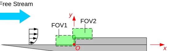
Figure 2. The field of views (FOV1 & FOV2) in the present experiment and the coordinate system.

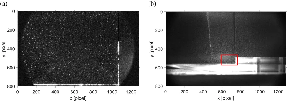
Due to the large distance between camera and the measurement plane, about 500mm, the conventional zoom lens is not able to visualize the flow details with sufficient spatial resolution. An Infinity K2 Distamax long-range microscope is thus used to deliver high resolution imaging. The present field of view (FOV) and the FOV acquired by a lens of 135 mm focal length are compared in figure 1. It can be seen that the present FOV has much higher magnification, thus allows resolving the smaller scale flow structure. Two field of views (FOVs) are arranged in the experimental campaign, one is located at the immediate upstream of the step, while the other is downstream, as depicted in figure 2. Both FOVs have the same size of 26.0 mm 17.3 mm (L H), thus a resolution of 21.6 µm/pixel is achieved, corresponding to a magnification factor of 1.08.

The laser pulse separation is chosen to be 15 µs for FOV1 and 10 µs for FOV2. The particles in the free stream thus have displacement of about 15 pixels in FOV1 and 10 pixels in FOV2. The data ensembles for FOV1 and FOV2 have 1000 pairs of particle images, respectively, corresponding to a measurement duration of 1 s. The image pre-processing procedure contains minimum background subtraction and particle smoothing using Gaussian kernel of 5x5 pixels. The velocity vector is calculated through cross-correlation using Window Deformation Iterative Multigraid (WIDIM) algorithm [10]. The initial interrogation window size is chosen 64x64 pixels. The final interrogation window size is 24x24 pixels with 50% overlap. The velocity vector fields are further validated using median test, through which the bad vectors are identified and re-interpolation from surrounding vectors. The final vector field has a total of 83x39 vectors with vector spacing of 0.25 mm, which defines the special resolution of the FFS measurements. The experimental setup as well as the PIV parameters are summarized in table 1.

Table 1. Parameters for experimental setup

Parameter Quantity

Flow speed 20 m/s

FOV Area ( ) 26.0 x 17.3 mm2 Magnification factor M 1

Particle diameter ~ 1

Laser pulse separation 15 µs (FOV1) 10 µs (FOV2) Particle displacement in free

stream ∆L ~ 15 pixel ~ 10 pixel

Ensemble size N 1000

Final interrogation window 24x24 pixel

Vector spacing 0.25 mm

3. RESULTS

3.1 Boundary Layer

to resolve into the viscous layer in the turbulent boundary layer. The log regime extends from y+ ≈ 20-200. The inflow condition is summarized in table 2.

Figure 3. The boundary layer at x/h=-3 in wall unit.

Table 2. Properties of incoming boundary layer

Parameter Quantity

Thickness 10 mm

Friction velocity 0.37 m/s

Reynolds number Reh 13,700

3.2 The Mean Flow

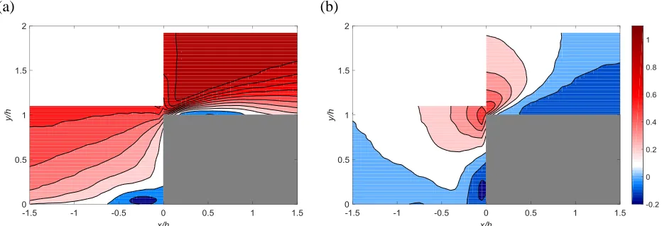
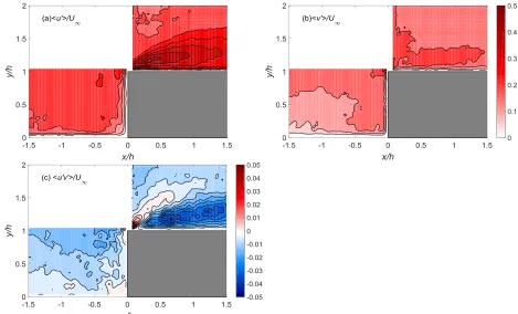
The mean flow is calculated by averaging the entire data ensemble containing 2000 uncorrelated snapshots. The contours of both the streamwise and wall-normal components provide an overall understanding of the resulted flow field. Two regions of flow separation are present in the immediate upstream and downstream of the step, respectively, see figure 4(a). The upstream one has a length of 0.6h, while the downstream one has a longer length of about 1h. However, the strength of the negative velocity is stronger at the foot of the step and that over the step is slightly weaker. Apart from flow separation, a focused shear layer is produced over the downstream separation bubble, it obtains rather strong velocity gradient within a thickness of about 0.3h. Due to the flow recirculation at the step foot, downward motion is present, see figure 4(b). The flow exhibits a peak upwash magnitude of 0.5U∞ at the tip of FFS, after

which it moves downward over the step.

(a) (b)

Boundary layer separation and redevelopment are better revealed through the velocity profiles. The profile at x/h=-1.0 deviates significantly from the turbulent boundary layer due to the adverse pressure gradient produced by the step. Separation can be observed in the profiles at x/h=-0.5 and -0.1. Boundary layer recovery takes place after separation in the immediate downstream of the step leading edge. The flow becomes attached at x/h=1.0, but the profile deviates significantly from the fully developed boundary layer.

Figure 5. Evolution of mean boundary layer profiles: (a) profiles upstream of the step; (b) profiles downstream of the step.

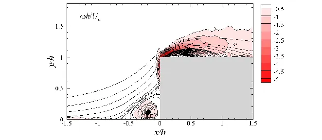
Figure 6. Contour of mean vorticity with streamlines showing the separation bubble.

The time-averaged vorticity field is calculated and plotted in figure 6, where streamlines is also overlapped to visualize the two separation bubbles. It can be found that the peak vorticity at upstream overlaps with flow recirculation. Much stronger vorticity is generated downstream of the step and the peak is found close to the step leading edge, which is about 5 times of the upstream magnitude. However, the peak value of the vorticity field in the downstream portion does not overlap with the downstream separation bubble, instead it follows the curved shear layer above the separation bubble.

3.3 Turbulent Properties

flow, although 〈 〉 is slightly stronger above the step. The Reynolds shear stress represents the turbulent shear activity in the flow field. Big difference in the shear intensity exists in the two parts of the flow field, see figure 7(c). The peaks of ̅̅̅̅̅ over the step has a much larger magnitude than that at the step foot. The strong negative peak at downstream is associated with the turbulent shear layer revealed earlier and suggests unsteady vortical activity in that region.

Figure 7. Contours of velocity fluctuations and Reynolds shear stress: (a) streamwise component

〈 〉 ⁄ , (b) wall-normal component 〈 〉 ⁄ . (c) Reynolds shear stress ̅̅̅̅̅ ⁄ . 3.4 Instantaneous Flow

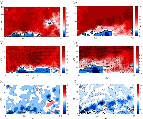
The instantaneous flow field differs from the time-averaged one due to the turbulent nature of the present flow. Since much higher fluctuation intensity was revealed in the flow field downstream of the step, the flow in that part is discussed first in this section. Snapshots of the instantaneous flow field represented by the streamwise velocity component is shown in figure 8. Separation bubble can be observed in the two snapshots, however its shape and area vary greatly. The shear layer at the interface between the free stream and separation is unstable and subject to undulation. Above the undulated shear layer, intermittent packets containing high streamwise velocity magnitude is produced, which is a clear indication of vortex shedding along the shear layer. The dimension of those packets is small, about 1 mm in diameter, and it is generated by the local acceleration of embedded vortex. Following the local vortical motion, flow in the opposite side of the shear layer is decelerated. As the shear layer undulates in different snapshots, the vortex train also moves in wall-normal direction, resulting in strong flow fluctuation, which explains the high magnitude of pressure fluctuations in the previous studies.

(a) (b)

(c) (d)

(e) (f)

Figure 8. The instantaneous flow fields downstream featured by streamwise velocity component ⁄ (a,b,c,d) and vorticity ⁄ (e,f). The flow field in (c) and (d) is close-up view in (a) and (b) respectively. Note that (a) (c) (d) belong to one snapshot, and (b), (d) and (f) belong to another uncorrelated snapshot.

(a) (b)

(c) (d)

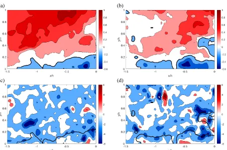
Figure 9. The instantaneous flow fields upstream of the step represented by streamwise velocity component ⁄ (a,b) and vorticity ⁄ (c,d). The ⁄ velocity contour line is overlaid using solid line.

3.5 Statistical Analysis

3.5.1 Statistics of flow separation

The flow separations taking place upstream and downstream of the step have been discussed respectively in the previous sections. Due to their nature of high unsteadiness, it is important to provide further statistics on the occurrence of separation area. The probability of occurrence of reversed flow is calculated and shown figure 10. Higher probability (>0.7) can be observed closer to the mean separation location, which is at the step foot for upstream separation and at x/h=0.5 for downstream separation. The area of front separation grows with decreased probability. The start point moves upstream while the tip point lifts closer to the top of the step. The area of the rear separation also grows with decreasing probability, however at a smaller rate than the front separation.

Figure 11. Probability of vortex generation, threshold value of is chosen for vortex identification. The probability of vortex generation is also studied as the vortical activity is not trivial in the FFS flow, especially in the region downstream of the step. Vortex identification is based on a threshold value of normalized vorticity magnitude, which is chosen to be 10, the averaged value for the vortex downstream of the step. Note that the sign of the vorticity is negative, the present discussion only concerns its magnitude. As it was revealed that the vortex upstream of the step has smaller vorticity, and the present criterion only detects very strong vortex in the upstream portion. Significant contrast in the probability of vortex generation is shown in figure 11. Vortex with high intensity, namely larger than , is produced with very low probability (<0.1) upstream of the step and it only occurs right at the foot region. On the contrary, such strong vortex is produced under much higher probability, with peak value of about 0.6 close to the step leading edge. Moreover, the high concentration of downstream vortex generation follows the shear layer instead of overlapping with the recirculation centre.

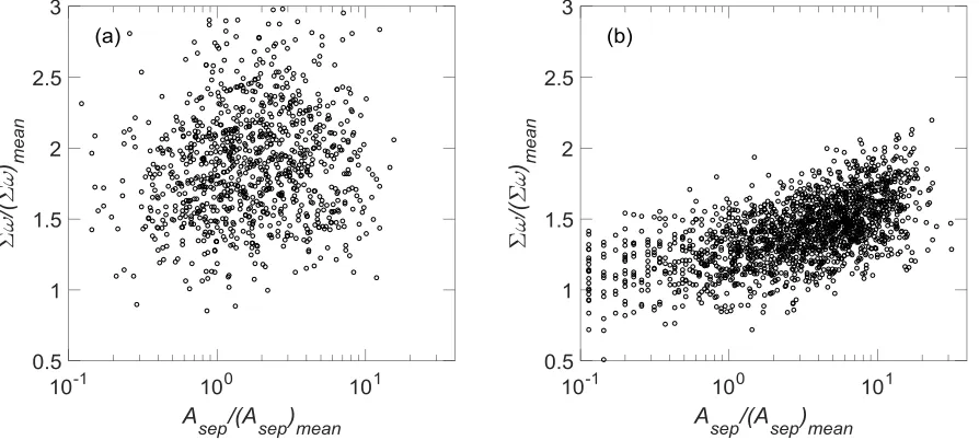
Flow separation and vortex generation have been investigated independently, they are now studied jointly so as to reveal the correlation between the two important flow structures in the FFS flow. The separation area and total vorticity magnitude are scatter-plotted in figure 12, intending to reveal their correlation. Note that both the separation area and total vorticity in the FOVs are normalized with the values in the mean flow field. It is rather clear that the increase of flow separation follows closely with the growing vorticity magnitude for the downstream flow. So far, it can be concluded that the strong link between them. The upstream portion, see figure 14(b), does not show any correlation between the two quantities.

4. Conclusions

The present PIV technique using long-range microscope has been implemented to visualize the FFS flow with high resolution. Two separation bubbles in the immediate upstream and downstream of the step are revealed. A strong shear layer is produced between the downstream separation and the free stream. The flow is subject to unsteadiness. The RMS of streamwise velocity components reveals that the streamwise velocity component exhibits much stronger intensity in the downstream portion than that upstream of the step, which is later attributed to the coherent vortical activity taking place along the unsteady shear layer. The correlation between the vorticity magnitude and area of separated flow is finally confirmed in the region downstream of the step, suggesting that the separation is likely to be caused by the vortex.

The distinctive features in turbulent and vortical activities for two flow regions, namely upstream and downstream of the step, indicates that the downstream flow dominates FFS flow in flow unsteadiness and more attention dedicated to the downstream portion would help solve the problems summarised in the introduction.

REFERENCES

[1] M Ji & M Wang (2010). Sound generation by turbulent boundary-layer flow over small steps. J. Fluid Mech., 654:161-193.

[2] M Costanitini, S Risius & C Klein (2015), Experimental investigation of the effect of forward-facing steps on boundary layer transition, IUTAM ABCM Symposium on Laminar Turbulent Transition, Procedia IUTAM, 14:152-162

[3] W Moss & S Baker (1980) Re-circulating flows associated with two-dimensional steps, Aeronautical Quarterly, 32:693–704.

[4] M Sherry, D Jo Jacono & J Sheridan (2010) An experimental investigation of the recirculation zone formed downstream of a forward facing step, J. Wind Eng. Ind. Aerodyn, 98:888-894.

[5] DJJ Leclercq, MC Jacob, A Louisot & C Talotte (2001), Forward-Backward facing step pair: aerodynamic flow, wall pressure and acoustic characterization, AIAA paper 2001-2249.

[6] Y Addad, D Laurence, C Talotte & MC Jacob (2003), Large eddy simulation of a forward-backward facing step for acoustic source identification, Int. J. Heat Fluid Flow, 24:562-571.

[7] JF Largeau & V Moriniere (2007) Wall pressure fluctuations and topology in separated flows over a forward-facing step, 42:21-40.

[8] R. Camussi, M Felli, F Pereira, G. Aloisio & A Di Marco (2008) Statistical properties of wall pressure fluctuations over a forward-facing step, 20:075113.

[9] CJ Kahler, R McKenna & U Scholz, Wall-shear-stress measurements at moderate Re-numbers with single pixel resolution using long distance PIV – an accuracy assessment, 6th International Symposium on Particle Image Velocimetry, Pasadena, CA, USA.