CFD modelling coupled with floating structures and mooring dynamics for offshore renewable energy devices using the Proteus simulation toolkit

CFD Modelling coupled with Floating

Structures and Mooring Dynamics for

Offshore Renewable Energy Devices using

the Proteus Simulation Toolkit

Tristan de Lataillade

, Aggelos Dimakopoulos

, Christopher Kees

,

Lars Johanning

, David Ingram

, Tahsin Tezdogan

∗_{Industrial Doctoral Centre for Offshore Renewable Energy, Edinburgh, UK}

(author for correspondence: [email protected]) †_{HR Wallingford, Howberry Park, Wallingford, UK}

‡_{Coastal and Hydraulics Laboratory, US Army ERDC, Vicksburg, USA}

§_{University of Exeter, College of Engineering, Penryn Campus, UK} ¶_{The University of Edinburgh, School of Engineering, Edinburgh, UK}

k_{University of Strathclyde, Department of Naval Architecture, Glasgow, UK}

Abstract—In this work, the coupling of novel open-source tools for simulating two-phase incompressible flow problems with fluid-structure interaction and mooring dynamics is presented. The open-source Computational Fluid Dynamics (CFD) toolkit Proteus is used for the simulations. Proteus solves the two-phase Navier-Stokes equations using the Finite Ele-ment Method (FEM) and is fully coupled with an Arbitrary Lagrangian-Eulerian (ALE) formulation for mesh motion allowing solid body motion within the fluid domain. The multi-body dynamics solver, Chrono, is used for calculating rigid body motion and modelling dynamics of complex mooring systems. At each time step, Proteus computes the forces from the fluid acting on the rigid body necessary to find its displacement with Chrono which will be used as boundary conditions for mesh motion. Several verification and validation cases are presented here in order to prove the successful coupling between the two toolkits aforementioned. These test cases include wave sloshing in a tank, floating body dynamics under free and wave-induced motion for different degrees of freedom (DOFs), and mooring dynamics using beam element theory coupled with rigid body dynamics and collision detection. The successful validation of each component shows the potential of the coupled methodology to be used for assisting the design of offshore renewable energy devices.

Index Terms—Computational Fluid Dynamics, Fi-nite Element, Fluid-Structure Interaction, Offshore Renewable Energy, Mooring Dynamics

I. INTRODUCTION

Being able to understand and predict the be-haviour of offshore floating structures under typical or extreme environmental loads is an important factor for assessing their viability. This becomes

particularly critical for offshore renewable energy where devices are purposely placed in highly ener-getic sites in order to capture a relatively abundant resource. Some of these floating devices aim to limit the response to wave loads such as floating wind turbines, while others are tuned to have a high response with the most energetic waves such as wave energy converters. The numerical tools used for simulating such events must be thoroughly verified and validated through established benchmarks, con-ceptual problems and comparison to experimental data from well monitored physical experiments.

Numerical modelling is rapidly and increasingly becoming cost and time efficient, and recent ad-vancements in this domain have made it more reli-able. These scientific efforts have led the world of Computational Fluid Dynamics (CFD) that tradition-ally preferred the Finite Volume Method (FVM) to look at the more flexible but more computationally expensive Finite Element Method (FEM).

Proteus, an open-source computational methods and simulation toolkit developed by the Engineer Research and Development Center (ERDC) of the U.S. Army Corps of Engineers (USACE) and HR Wallingford, is used in the work presented here for solving Navier-Stokes equations, tracking the free surface of two-phase flows, and moving the mesh. The source code of Proteus is available to all at: https://github.com/erdc-cm/proteus.

This library allows a fully coupled simulation of rigid and flexible bodies with FEM cable dynamics, where collision detection of the cables with struc-tures is enabled by creating node clouds along the cable. The source code of Chrono is available at: https://github.com/projectchrono/chrono

The focus of the research presented here is the simulation of wave-structure interaction coupled with floating rigid body and mooring dynamics using novel open-source tools. First, the capabilities of the CFD solver alone for simulating two-phase flows are presented with a conceptual model of wave sloshing motion in a fixed tank. Then, numerical results for floating bodies are validated against experimental data for different degrees of freedom (DOF). This includes free oscillation and decay of surface-piercing bodies released from a position away from equilibrium, and wave-induced oscillation under wave loads of various frequencies. Finally, mooring quasi-statics and mooring dynamics coupled with rigid body motion will be presented.

II. GOVERNINGEQUATIONS

A. Fluid Domain

In the context of the simulations presented in following sections, the fluid domainΩf is composed

of two phases: the water phase (Ωw) and the air

phase (Ωa), so thatΩf = Ωw∪Ωa. Solution within Ωf is computed with Proteus in the following steps.

1) Navier-Stokes: The fluid velocity field is obtained through the Navier-Stokes equation for incompressible fluid (see eq. (1)).

(

ρu˙ +ρu· ∇u− ∇ ·σ¯¯ =ρg

∇ ·u= 0 (1)

with the density of the fluid ρ, the fluid velocity vector u, the gravity acceleration vector g, and the Cauchy-Schwarz tensorσ¯¯ =−pI+µ∆uwith pressurepand dynamic viscosityµ.

Dividing by the density, the first term of eq. (1) is often written as:

˙

u+u· ∇u− ∇ · ν ∇u+∇ut=g−1

ρ∇p (2)

With kinematic viscosityν= µ_ρ

The time integration used for the cases presented here is backward Euler due to its robustness and lower computational cost when compared to higher order methods. The Courant-Friedrichs-Lewy (CFL) condition is used to limit the size of the time step (eq. (3)).

CFL=u∆t

∆x (3)

where∆tis the time step and ∆xis the character-istic element length. The CFL value is calculated

for each cell, and is limited against a predefined value throughout the numerical domain.

2) Free Surface Tracking: The free surface is de-scribed implicitly using the Volume-of-Fluid (VOF) [5] method coupled with the Level Set (LS) method [12]. The LS method uses a signed distance function as shown in eq. (4), giving the distance of any point in space φfrom the free surface.

(

k∇φk= 1 ∀x∈Ωf

φ= 0 ∀x∈Γaw

(4)

The VOF method returns 0 for all points in the water phase, 1 for all points in the air phase, and values between 0 and 1 in a transition zone around the free surface using a smoothed heaviside function (see eq. (5)).

θ(φ) =    

  

0 φ <−

1 2

1 + φ +1 πsinφπ

|φ| ≤

1 φ >

(5)

Whereis a user defined smoothing distance (equal to 3 characteristic element length throughout this paper), andθ the value of the heaviside function.

The LS model is used to correct the VOF model, more details about this implementation are available in [11].

3) Turbulence: In Proteus, the Navier-Stokes equation are discretised in space using Residual-Based Variational Multiscale (RBVMS) method, as originally proposed in [2] and there are 2 turbulence models available: k-and k-ω.

B. Body Dynamics

As mentioned previously, Project Chrono – an open-source multi-body dynamics simulation engine – is used for the simulation of floating bodies presented in this work. It allows the simulation of rigid and flexible bodies, imposition of constraints (joints, springs, etc.), and collision detection, as well as finite element modelling of beams and cables (more details about the latter in sectionIV-C).

To define a rigid body, the necessary variables are its massm, inertia tensorIt¯¯ (2×2in 2D,3×3

in 3D), and the original position of its barycentrer0. In addition, the geometrical description of the outer shell of the body must be provided using vertices, segments, and facets, as the mesh on the exterior surface of the body conforms to the fluid mesh, while the interior of the body (Ωs) is not mesh as

the structures investigated in this work are assumed fully rigid.

The hydrodynamic forces over the fluid/solid interface, ∂Ωf∩s = ∂Ωf ∩ ∂Ωs, is computed

from the solution of the Navier-Stokes equations. Subsequently, stresses are integrated over the body boundaries to provide forcesFf and momentsMf as described in eqs. (6–7).

Ff= Z

∂Ωf∩s

¯ ¯

σndΓ (6)

Mf= Z

∂Ωf∩s

(x−r)×( ¯σ¯n)dΓ (7)

withnnormal vector to the boundary, x a point on the boundary,rthe position of the barycentre, and

Γthe boundary (segment if 2D, surface if 3D). The total forces and moments are then used to calculate the new acceleration, velocity, and position of the body for a given time step (see eqs. (8–9)).

Ft=m¨r (8)

Mt= ¯It¯ω˙ (9)

with m the mass,It¯¯ the inertia tensor and ω the angular acceleration of the body.

The time integration chosen for solving body dynamics in the simulations presented here is implicit Euler for systems of second order using the Anitescu/Stewart/Trinkle single-iteration method. Other integration methods are available in Chrono, and this one was chosen for its robustness and speed. Because a time step within Chrono takes much less computational time than a time step of Proteus, the rigid body solver uses several substeps with the CFD solver time step, allowing a more refined solution for body dynamics.

C. Mesh Motion

In Proteus, the mesh is moved using the Arbitrary Lagrangian-Eulerian (ALE) method also known as the Mixed Interface-Tracking/Interface-Capturing Technique (MICTICT) [16].

The mesh motion is solved through the equations of linear elastostatics, which take the form of eq. (10) for the equilibrium equation.

f+µ∇2_{u+ (λ+µ)∇(∇ ·u) = 0 (10)}

whereλandµare the Lam´e parameters, as shown in eq. (11).

µ= E

2(1 +ν) (11)

λ= µE

(1 +ν)(1−2ν) (12)

For the simulations presented in this work, the nominal mesh Young’s modulus is E = 1 and Poisson ratio isν = 0.3.

Fig. 1: Snapshots of mesh deformation around moving body for different positions (top left shows the mesh as it was initially generated).

The mesh is constrained, in our case, at the borders of the domain (walls and solid boundaries) and is updated at each time step by using the displacement of the nodes at the boundary of the rigid bodies. The mesh then deforms in the fluid domain following eq. (10).

The mesh motion is taken into account directly in the Navier-Stokes equations that are solved in the Eulerian frame. This is achieved by solving the equation in a transformed space, where the mesh motion effect is introduced as an additional transport term in the conservation equations [1].

The displacement of the nodes placed on a mov-ing body are used as dirichlet boundary conditions for the moving mesh model, and are obtained through eq. (13).

∆xn = xn−xnp

·Rn+1−(xn−xnp)+h n+1

(13)

withxthe coordinates of a point in space, xp the

coordinates of the pivotal point (which is the centre of mass in the case of a single body not experiencing any collisions),hthe translational displacement, and Rn+1 _{the rotation matrix of the body from its}

position at time tn _totn+1_.

At the tank/domain boundaries (∂Ω), the mesh nodes are either fixed ((∆xn_{) = 0) or are allowed}

only a translational motion along the boundary (∆xn·n= 0).

Figure 1illustrates a close-up the moving mesh around a moving body.

Additional details about the mesh motion are provided in [1].

III. VERIFICATION ANDVALIDATION

A. Sine Wave Sloshing

This verification test case looks at spatial and temporal convergence of the solution of a conceptual two-phase flow problem in the absence of any moving obstacle, meaning that the mesh motion module is not activated.

The sloshing motion of a body of water is studied in a fixed tank given initial conditions for the free surface. This type of test case is common practice for verifying that the coupling of the equations of two-phase flow CFD solvers work adequately, and to quantify their accuracy and convergence order. The conditions used are the same as in [14] (based on [17]), with a 2D tank of dimensions0.1×0.1m, water depth d = 0.05m, and amplitude of the sinusoidal profile of the free surface ofa= 0.05m. The initial conditions are derived using the third order solution as provided by [15] for a sloshing wave of the first mode in a fixed tank. This analytical solution is also used as a comparison to the time-varying numerical results. Boundary conditions are free-slip on the tank bottom and side walls and atmospheric conditions at the top boundary. In this conceptual model, the fluid viscosity is turned off (ν = 0). For all test cases, the mesh used is unstructured with triangular elements that are of the same size all across the domain.

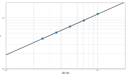
The error between the numerical results and theoretical curve is estimated using Pearson product-moment correlation coefficient (PPMCC or Pear-son’s r) over the first 5 periods of the sloshing oscillation.

On fig. 2, the error of the pressure obtained numerically at the left boundary placed halfway in the water column is plotted for different time stepping. The order of convergence can be found by fitting a linear curve to the error data on a logarithmic scale. It clearly appears that the solution converges with, in this case, a convergence order of 0.8 for time convergence with a fixed mesh refinement with characteristic element size ofhe= ₁₀a. Varying the spatial refinement also has

an effect, but tests shows that it becomes minimal when compared to reducing the time step after a sufficiently refined mesh value (herehe= ₁₀a). The variation of the CFL value instead of using fixed time step also gives an order of convergence of 0.8, but the solution gets away from the asymptotic range for a CFL value superior to 0.5. For this reason, the simulations presented in the next sections of this paper use CFL<0.5.

B. Floating Body - Free Oscillation

This section presents validation results for floating bodies with different constraints on their degrees of freedom.

Fig. 2: Error () between numerical results and an-alytical solution for pressure sloshing wave motion using PPMCC on the 5 first periods for different fixed time steps (∆t).

1) Roll: This experiment is based on the ex-perimental setup of [10] with a floating caisson of dimensions 0.3m×0.1m (length×height) that is constrained for all DOFs apart from roll, in a tank of dimensions35m×1.2m. The width of the caisson and the tank are the same: 0.9m, making it possible to approximate the experiment numerically by setting a 2D test case, where a slice of the experimental setup can be used numerically. The width of the caisson is only taken into account when calculating the forces and resulting moments on the floating body using its moment of inertia Izz= 0.236kg m2.

The initial conditions are as follows: initial angle of15◦ for the floating caisson, tank of total dimensions 5m×1.8m with absorption zones of

2mat each end of the tank, and fluid at rest with a water column of 0.9m. For this experiment, no-slip boundary conditions (dirichlet value of zero for all velocity components) were imposed on bottom and side walls (Γwall) of the tank and on all facets

of the caisson. The top boundary (Γatm) of the

tank used atmospheric conditions, with dirichlet boundary conditions preventing fluid to travel in a motion parallel toΓatmand a VOF value imposed

as the value of air (1 in this case). The simulated time was as long as the experimental recordings: 5 seconds.

Fig. 3: Time series of roll motion of rectangular (2D) floating body forhe=H20c (withHc the height

of the floating body) and fixed∆t= 5e−4 with initial angleφ0= 15◦. Experimental results were

digitalised from [10].

the tank are the same, the 2D numerical simulation is just a slice of a 3D experimental setup (the latter inevitably letting some fluid travel across the width of the tank). Furthermore, the turbulence model was switched off during the simulation, similarly to the particle-in-cell simulation of the same case from [3] that gives similar results to Proteus in terms of damping of the oscillation.

In order to investigate the stability of the mesh motion integrated in Proteus, the natural period was also calculated for different starting angles (5◦,

10◦,15◦) that lead to different mesh deformations. This resulted in a maximum difference of 0.2% between the results for the natural period of the rolling caisson with different initial angle and similar damping profiles, proving the robustness of the ALE mesh technique. The small difference could be explained by nonlinearities developing in the fluid domain and affecting the motion slightly due to the difference of volume of water displaced and velocity/vorticity of the fluid around the floating body when using different starting angle.

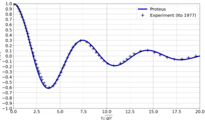
2) Heave: This test is based on the experiment of [6], where the heave oscillation of a cylinder was studied with: cylinder length ofL= 1.83m and a diameter ofD= 15.24cm (with1.27cm between the tank walls and end-plates of the cylinder). The cylinder is halfway submerged when at rest, and all DOFs apart from heave are constrained.

For this simulation, the initial conditions are similar to the previously described test case with the fluid at rest and no-slip boundary condition and cylinder is pushed down from its resting position to a given initial position (−2.54cmfrom still water level). The mesh refinement is as follows: constant mesh refinement up to a distance equal to the initial push of the cylinder around the mean water level, and up to a distance ofD from the cylinder boundaries. Gradual coarsening of the mesh is then

Fig. 4: Time series of heave motion of a circular (2D) floating body forhe= ₅₀d and fixed∆t= 5e− 4with initial push ofy0=−2.54cm. Experimental

results were digitalised from [6].

applied from the refined parts with 10% increase in area of mesh elements.

A time series of the experimental and numer-ical results is presented in fig. 4, with the time normalised as tpg

r, and the heave displacement

normalised as _yy

0. The numerical curve is in good agreement with the experimental curve, leading to accurate prediction of the natural period and of the damping of the oscillation. Even though the DOF investigated here is different, one could argue that the good agreement obtained in damping could mean that there was indeed frictional effects in the experiment described in the previous section, where the experimental damping was overestimated.

C. Floating Body - Wave-Induced Oscillation

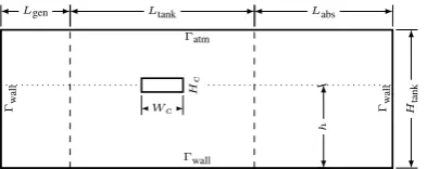
In this experiment, still based on the experimental setup [10] with a configuration similar to the one described in section III-B1, waves are generated in order to compute the Response Amplitude Operator (RAO) of the floating body. With λthe wavelength of the wave generated, the tank dimensions are changed depending on the wave characteristics in order to match a generation zone of 1λ to limit wave reflection upstream and an absorption zone of

2λto absorb waves downstream. The two relaxation zones are separated by a distance of 2λ, and the floating body is placed1λaway from the generation zone (see fig. 5). Initially, the floating body is at rest position (no initial rotation).

As the waves generated for this example are weakly nonlinear, their profile is computed using the Fenton approach with Fourier Transform in order to get a wave profile close to fully developed. See tableIfor the characteristics of the waves generated. For each test case, the characteristic element size was no less than he = ₂₀₀λ . The generation and

Lgen L_tank L_abs

H

tank

Γatm

Γwall

Γw

all

Γw

all

Wc

H

c

h

Fig. 5: Numerical tank setup for a typical floating body test case under wave loads.

Figure6gives results for the response of the body under different wave frequencies and amplitudes plotted against the experimental results and linear theory. Overall, these results are in good agreement with the experimental results, as explained in more details below.

For higher frequency waves, where _ωω n > 1, the results are in good agreement with the linear potential theory as well as the experimental results. At _ωω

n = 1.15, where the experiment shows a smaller response than the theory, the divergence in response between the experiment and the nu-merical/theoretical results looks particularly large, possibly due to the steepness of the response curve at this particular point, meaning that even a small difference of wave frequency between the experimental setup and the numerical setup could lead to a very different response result. At

ω

ωn = 1.32, 3 tests with same frequency waves but different wave heights were run, and similar results were obtained, confirming the experimental observations that the wave height has a negligible effect on the caisson response at high frequency.

For waves with frequency identical to the natural frequency of the caisson (_ωω

n = 1), the magnifi-cation factor varies greatly with wave height. The numerical results for different wave heights shown in fig.6at _ωω

n = 1 indicate that the magnification value increases when the wave height decreases, which is the expected behaviour according to [10].

For lower frequency waves (_ωω

n <1), the numer-ical results are generally closer to the experimental results than the linear potential theory. This can be explained by the fact that nonlinearities have a significant effect at these frequencies, affecting the caisson response. The numerical results, however, seem to slightly underestimate this effect when compared to the experiment. Possible reasons for this behaviour include the rather large characteristic element size (with respect to the floating body dimensions) for longer wave periods (asheis scaled

with λ) and/or the larger time stepping. It is worth noting that results from [3] using PICIN (Particle In Cell - INcompressible) for this case are different in this frequency range with an overestimation

Fig. 6: RAO of rolling caisson under regular wave loads, withφthe roll response,k the wavenumber, andA the wave amplitude

of the nonlinear effects when compared to the experiment. Further investigation is necessary, with a finer mesh around the caisson as these low wave frequencies lead to relatively large wavelengths and the characteristic element size was scale with the wavelength throughout the whole domain for these simulations. Figure7shows snapshots of the floating body oscillation and fluid velocity and direction for a full wave period in the case of _ωω

n = 0.77. IV. MOORINGS

Moorings are an important component of floating offshore renewables that should not be overlooked as it can significantly influence the response of the device. This section presents a quasi-statics module that was developed independently and validation of mooring cable dynamics using the Project Chrono library. The quasi-statics model is used for setting initial conditions to lay out the mooring cables for the dynamics model.

A. Quasi-Statics

The quasi-statics module developed here supports multi-segmented sections (line made out of different materials) and stretching of the cable is taken into

TABLE I: Wave characteristics for computing RAO of floating body (see fig.6)

(a) (b)

(c) (d)

(e) (f)

(g) (h)

(i) (j)

(k) (l)

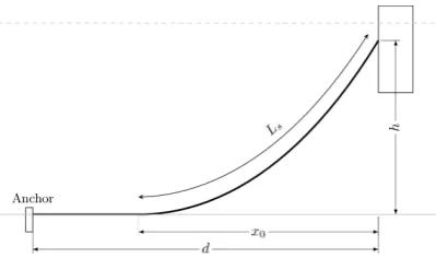
Fig. 8: Catenary layout, withx0the horizontal span,

Lslifted cable length,dhorizontal distance between

anchor and fairlead,hvertical span

account. It is also used for initial conditions in order to lay out the cable given fairlead and anchor coordinates, and the length of the cable.

Once the shape of the catenary described with the parameter a is found (see fig.8 for a typical catenary layout of a mooring line), the catenary equation eq. (14) can be used to find coordinates of points along the cable.

y=acoshx

a

(14)

s=asinhx

a

(15)

withy the vertical position (direction aligned with the gravitational acceleration), x the horizontal position,sthe distance along the cable, and athe characteristic value of the catenary shape.

In the current implementation of the quasi-statics module, an iterative process is used. In case of a partly-lifted line, the right value of the horizontal spanx0 of the mooring line must be found so that

the lifted line length and the line laying on the seabed are together equal to the total line length. If the line is fully lifted (Ls=L), a transcendental

equation inais solved (see eq. (16)).

p

Ls2_−h2_{= 2asinh} d

2a (16)

If elasticity of the line is taken into account, more iterations are needed to adjust the change in lifted line length as it stretches.

Quasi-statics analysis can be used to estimate the order of magnitude of tensions that are experienced by the floating device. It is a simple and fast method, but it neglects the dynamic effects of the cable that can become non-negligible under certain conditions (e.g. wave frequencies applying large and varying loads on the device), often leading to an underestimation of the maximum tensions that can occur along the cable.

This module can be used for simple and fast moorings analysis, but also for initial conditions

Fig. 9: validation of quasi-statics module for dif-ferent surge positions of a WEC moored with 3 catenary lines, with x0 the horizontal span, d the

vertical and h the horizontal distance from the anchor to the fairlead, and T the tension at the fairlead.

to lay out cables at equilibrium position for a more complex and demanding dynamic analysis as described in the following section. Figure 9

shows results of a quasi-statics analysis compared to experimental results from [4], where a Wave Energy Converter (WEC) is moored with 3 catenary lines with 4 different segments each (2 chains and 2 ropes) and is placed at different surge positions.

B. External Forces

The total external force fe due to the fluid

surrounding the cable is:

fe=fd+fam+fb (17)

Withfd the drag force,fam the added mass force,

andfb the buoyancy force.

The buoyancy force is applied as a volumetric load and calculated as follows, with ρc the density

of the cable, and ρf the density of the fluid:

fb= (ρc−ρf)g (18)

The drag force and added mass force use dif-ferent coefficients for their tangential and normal components to the cable. The tangential and normal components of a vector are denoted withtandn in

the following equations, and can be found for any vector following eqs. (19–20).

xt= x·tˆtˆ (19)

xn=x− x·tˆ _ˆ

t (20)

fd=fd,n+fd,t (21)

fd,n= 1

2ρfCd,ndnkur,nkur,n (22)

fd,t= 1

2ρfCd,tdakur,tkur,t (23)

with Cdn andCdt the normal and tangential drag

coefficient,dn and da the normal and axial drag

diameters, andur the relative velocity of the fluid

to the cable element as in eq. (24).

ur=uf−r˙ (24)

The added mass force is calculated with the acceleration of the fluid with the cablear, as shown in eqs. (25–27).

fam=fam,n+fam,t (25)

fam,n=ρfCam,n

πd2

4 ar,n (26)

fam,t =ρfCam,t

πd2

4 ar,t (27)

For each element, the drag and added mass forces are calculated at the nodes and averaged to be applied as a distributed load over the length of the element.

As the mooring cable mesh and the fluid domain mesh do not conform, the loads can be calculated from the velocity and acceleration of the fluid at the nodes of the cable that can be retrieved from the fluid domain using the solution of the Navier-Stokes equations calculated from Proteus in each cell containing a cable node.

C. Dynamic Analysis

For mooring dynamics, the FEM method was used within Chrono. The cable is discretised in elements that are described with the Absolute Nodal Coordinate Formulation (ANCF). The ANCF beam elements are composed of 2 nodes, each defined with their position and direction vectors.

The mooring and floating body dynamics are fully coupled and solved together with Chrono between each CFD time step by applying the external forces computed from Proteus. Substeps within a main CFD step are generally used for stability and better accuracy of the multi-body dynamics as these are usually significantly cheaper computationally than when solving the equations for the fluid domain. In the current implementation, the external forces from Proteus computed for each CFD step are kept constant within the multi-body dynamics substeps. In the simulations presented here, the material of the mooring cables is assumed to be transversely isotropic. Bending stiffness can be changed by modifying the moment area of inertia, and collision

Fig. 10: Indicator diagram with axial pretension TA0 = 11.78N, ω = 0.79rad s−1 and a= 0.04z.

Experimental and Orcaflex results from [9].

detection of the cable with obstacles such as the seabed is activated by producing a nodes cloud.

Due to its relatively slender profile and to allow unrestricted displacement of the mooring line, the mooring cable has its own separate mesh. The slender profile of the mooring cable would require very small mesh elements relative to the rest of the domain, increasing the computational cost of the simulation drastically. Furthermore, the displace-ment of the cable within the fluid domain might be too large for the moving mesh to handle accurately.

In the current implementation, the fluid can act on the mooring (hydrodynamic loads as described in the previous section), but there is no feedback of the mooring displacement onto the fluid. The effects of the mooring cable on the fluid is thought to be negligible compared to the other forces in the simulation.

The test case chosen for validating the moorings dynamics is based on [8,9], where a scaled cylindri-cal floating Wave Energy Converter (WEC) and its catenary mooring line are modelled experimentally. The WEC is placed in a tank with uniform water depth of z = 2.8m and has a diameter of 0.5m

and height of 0.2m. Several weights of the WEC were tested, and the one used here to compare results is m= 30kg. The mooring line is a chain of length L= 6.98m with submerged weight per unit length of w = 1.036N m−1_{. The fairlead is}

placed h= 2.65m above the seabed. The chosen experiment consists in driving the WEC in the surge direction at a given angular frequency ω and amplitudeawith, in this case,a= 0.04z and w= 0.79rad s−1 _{with pretension T}

A0= 11.78N.

by retrieving the relative velocity of the cable with the fluid velocity. Figure10is an indicator diagram, showing the horizontal tension at the fairlead against the position in surge of the WEC. The tensions are well predicted with Chrono, and the dynamic effect (hysteresis of the curve) due to the drag force acting on the mooring line can be observed. The difference in hysteresis observed between Chrono and the experiment can be influenced by the drag and added-mass coefficients, which are derived from assumptions and are one of the main source of errors in mooring dynamics simulations. In this case, Cd,n = 1.4, Cd,t = 1.15, Cam,n = 1 and

Cam,t = 0.5 were used in Chrono, as they are

typical values used for studless chain. This is a work in progress and further testing with different coefficients is required.

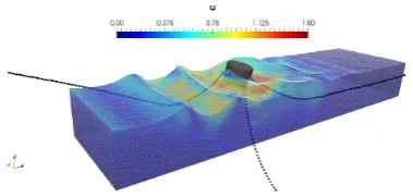
Preliminary simulations using all the tools pre-sented in this work – CFD with wave generation and ALE mesh, floating body and mooring dynamics, and collision detection – have been successfully produced and show great potential for simulating realistic cases for offshore renewable energy ap-plications. An illustrative snapshot of a 3D proof-of-concept simulation is shown in fig. 11 based on the floating cylinder and mooring configuration of [13], with 3 catenary mooring lines discretised with 100 elements per mooring cable, and regular wave generation with period T = 1s and height h= 0.15min a tank with a water level of 0.9m. For mooring cable nodes that extend outside of the CFD domain, fluid velocity is assumed to be the one given by the waves that are used as boundary conditions in the CFD model (assuming that the waves are then are undisturbed). As mentioned earlier, this is an early proof-of-concept simulation combining all the tools that have been validated in the work presented here, implying that further testing and validation of the models coupled together is necessary to more confidently use it as a whole for complex CFD simulations making use of floating body and mooring dynamics.

V. CONCLUSION

The numerical results presented in this paper for two-phase flows CFD using the Proteus toolkit coupled with body and mooring dynamics using the Chrono library show good agreement with a variety of analytical, numerical and experimental results. Temporal and spatial convergence of the two-phase flow solver alone was shown with the sloshing motion of a body of water, with error from the results laying in the asymptotic range. The simulation of floating bodies with Proteus and Chrono was undertaken for i) free oscillation for comparing their natural period and damping of the

Fig. 11: Snapshot of proof-of-concept simulation combining wave generation, ALE mesh, and 3 catenary mooring lines attached to a 6 DOF floating cylinder at t = 12.8s. Color map shows velocity magnitude.

simulation with experiments (roll and heave motion) and ii) the RAO of a floating body under loads of regular waves of different frequencies. Finally, the simulation of mooring lines with quasi-static and dynamic models was validated against experimental data.

The aforementioned test cases successfully demonstrate the capabilities of Proteus – an FEM based solver differing from the majority of the main open-source CFD tools that are FVM based – as a viable solution for modelling the key aspects of floating offshore renewable energy devices when coupled with Chrono. The combination of these numerical tools show great potential to reliably simulate the response of possibly complex offshore floating structures enduring environmental loads.

ACKNOWLEDGEMENT

Support for this work was given by the Engineer Research and Development Center (ERDC) and HR Wallingford through the collaboration agreement (Contract No. W911NF-15-2-0110). The authors also acknowledge support for the IDCORE program from the Energy Technologies Institute and the Re-search Councils Energy Programme (grant number EP/J500847/).

REFERENCES

[1] I. Akkerman, Y. Bazilevs, D. J. Benson, M. W. Farthing, and C. E. Kees. Free-Surface Flow and Fluid-Object Interaction Modeling With Emphasis on Ship Hydrodynamics.Journal of Applied Mechanics, 79(1), 2012.

[2] Y. Bazilevs, V. M. Calo, J. A. Cottrell, T. J R Hughes, A. Reali, and G. Scovazzi. Variational multiscale residual-based turbulence modeling for large eddy simulation of incompressible flows. Computer Methods in Applied Mechanics and Engineering, 197(1-4):173–201, 2007. [3] Qiang Chen, Jun Zang, Aggelos S. Dimakopoulos, David M.

Kelly, and Chris J K Williams. A Cartesian cut cell based two-way strong fluid-solid coupling algorithm for 2D floating bodies.Journal of Fluids and Structures, 62: 252–271, 2016.

[5] C.W Hirt and B.D Nichols. Volume of fluid (VOF) method for the dynamics of free boundaries. Journal of Computational Physics, 39(1):201–225, 1981.

[6] Soichi Ito.Study of the Transient Heave Oscillation of a Floating Cylinder. PhD thesis, 1977.

[7] Niels G. Jacobsen, David R. Fuhrman, and Jørgen Fredsøe. A wave generation toolbox for the open-source CFD library: OpenFoam.International Journal for Numerical Methods in Fluids, 70:1073–1088, 2012.

[8] Lars Johanning and George H Smith. Interaction Between Mooring Line Damping and Response. InInternational Conference on Offshore Mechanics and Arctic Engineering (OMAE), 2006.

[9] Lars Johanning, George H Smith, and Julian Wolfram. Measurements of static and dynamic mooring line damping and their importance for floating WEC devices. Ocean Engineering, 34:1918–1934, 2007.

[10] Kwang Hyo Jung, Kuang-an Chang, and Hyo Jae Jo. Viscous Effect on the Roll Motion of a Rectangular Structure.Journal of engineering mechanics, 132(2):190– 200, 2006.

[11] C. E. Kees, I. Akkerman, M. W. Farthing, and Y. Bazilevs. A conservative level set method suitable for variable-order approximations and unstructured meshes.Journal of Computational Physics, 230:4536–4558, 2011.

[12] Stanley Osher and James a. Sethian. Fronts propagating with curvature dependent speed: Algorithms based on Hamilton-Jacobi formulations.Journal of Computational Physics, (1988):12–49, 1988.

[13] Johannes Palm, Claes Eskilsson, Guilherme Moura Paredes, and Lars Bergdahl. Coupled mooring analysis of floating wave energy converters using CFD.International Journal of Marine Energy, 16:83–99, 2016.

[14] L Qian, D M Causon, D M Ingram, and C G Mingham. Cartesian Cut Cell Two-Fluid Solver for Hydraulic Flow Problems. Jounal of Hydraulic Engineering, (September): 688–696, 2003.

[15] Iradj Tadjbakhsh and Joseph B Keller. Standing Surface Waves of Finite Amplitude. (December), 1959.

[16] Tayfun E Tezduyar. Finite Element Methods for Flow Problems with Moving Boundaries and Interfaces. Com-putational Methods in Engineering, 8(September 2000): 83–130, 2001.