City, University of London Institutional Repository
Citation
: Goodwin, S., Dykes, J., Slingsby, A. & Turkay, C. (2015). Visualizing Multiple
Variables Across Scale and Geography. IEEE Transactions on Visualization and Computer
Graphics (Proceedings of the Visual Analytics Science and Technology / Information
Visualization / Scientific Visualization 2015), 22(1), pp. 599-608. doi:
10.1109/TVCG.2015.2467199
This is the accepted version of the paper.
This version of the publication may differ from the final published
version.
Permanent repository link:
http://openaccess.city.ac.uk/12337/
Link to published version
: http://dx.doi.org/10.1109/TVCG.2015.2467199
Copyright and reuse:
City Research Online aims to make research
outputs of City, University of London available to a wider audience.
Copyright and Moral Rights remain with the author(s) and/or copyright
holders. URLs from City Research Online may be freely distributed and
linked to.
City Research Online:
http://openaccess.city.ac.uk/
[email protected]
Visualizing Multiple Variables Across Scale and Geography
Sarah Goodwin, Jason Dykes, Aidan Slingsby and Cagatay Turkay
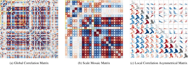
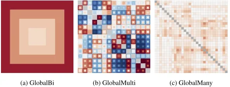
[image:2.612.111.510.121.259.2](a) Global Correlation Matrix (b) Scale Mosaic Matrix (c) Local Correlation Asymmetrical Matrix
Fig. 1: Multivariate comparison across scale and geography showing correlation through a red (positive) to blue (negative)
di-verging color scheme:(a)global correlation matrix;(b)scale mosaic matrix showing four levels of scale resolution (SR) within
a global correlation matrix (for a subset of variables),(c)geographical and statistical views in an asymmetrical correlation matrix
for a further subset reveals geographic variation in local correlation values (adaptive moving window –N= 25).
Abstract— Comparing multiple variables to select those that effectively characterize complex entities is important in a wide variety of domains – geodemographics for example. Identifying variables that correlate is a common practice to remove redundancy, but correlation varies across space, with scale and over time, and the frequently used global statistics hide potentially important differ-entiating local variation. For more comprehensive and robust insights into multivariate relations, these local correlations need to be assessed through various means of defining locality. We explore the geography of this issue, and use novel interactive visualization to identify interdependencies in multivariate data sets to support geographically informed multivariate analysis. We offer terminology for considering scale and locality, visual techniques for establishing the effects of scale on correlation and a theoretical framework through which variation in geographic correlation with scale and locality are addressed explicitly. Prototype software demonstrates how these contributions act together. These techniques enable multiple variables and their geographic characteristics to be consid-ered concurrently as we extend visual parameter space analysis (vPSA) to the spatial domain. We find variable correlations to be sensitive to scale and geography to varying degrees in the context of energy-based geodemographics. This sensitivity depends upon the calculation of locality as well as the geographical and statistical structure of the variable.
Index Terms—Scale, Geography, Multivariate, Sensitivity Analysis, Variable Selection, Local Statistics, Geodemographics, Energy
1 INTRODUCTION
The various ways that geographical phenomena interrelate with loca-tion and scale [1, 3, 11, 26] are at the core of geographical analy-sis. Despite this, multivariate geographical phenomena are frequently
studied usingglobal summary statistics that do not take geography
into account [13, 50]. Although these make results and analysis man-ageable, they hide important local variations in space, time, and scale. We investigate the effects of varying scale in multivariate compari-son, establish a complex parameter space for geographic analysis and present a new theoretical framework to manage these complexities. The framework allows multiple variables, and the relationships be-tween them to be visualized concurrently in the contexts of geography and scale. Just as visual parameter space analysis (vPSA) [38] ex-plores the effects of varying parameter values in a model parameter
• Sarah Goodwin is with Monash University and the giCentre, City University London. E-mail: [email protected].
• Jason Dykes, Aidan Slingsby, Cagatay Turkay are with the giCentre, City University London. E-mail:{J.Dykes, A.Slingsby,
Cagatay.Turkay.1}@city.ac.uk.
Manuscript received 31 Mar. 2015; accepted 1 Aug. 2015; date of publication xx Aug. 2015; date of current version 25 Oct. 2015. For information on obtaining reprints of this article, please send e-mail to: [email protected].
space, we explore the parameters of geography and scale. By applying existing vPSA techniques and terminology to this context, we estab-lish the construct of geo-visual PSA (gvPSA).
To demonstrate the applicability of the framework we apply it to the selection of variables for use in a geodemographic classifier focused on UK domestic energy consumption. Household energy is particu-larly relevant in this context as consumption is known to be highly geographical, but varies with the socio-economic characteristics of the population [8]. Our work with energy analysts identifies a need for better energy consumer profiling in the UK as well as the benefit of specifically designed visualization [15].
Appropriate variable selection is important in achieving valid and
discriminating geographical profiles [49]. Standard practice is to
avoid variables that may bias clustering results – such as those that
strongly correlate or are heavily skewed. Variable selection is a
well researched topic in the visualization and machine learning lit-erature [17, 25, 29, 32, 39, 45]. However, geographical aspects of these variables and their interactions with each other are not usually considered and where variables interact not only with each other but also with underlying geography, an algorithmic approach is not always sufficient [33].
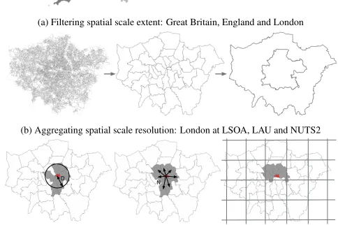
(a) Filtering spatial scale extent: Great Britain, England and London
(b) Aggregating spatial scale resolution: London at LSOA, LAU and NUTS2
D
N
(c) Locality definitions using ‘City of London’ (red) as a starting location:fixed(by
[image:3.612.48.290.129.290.2]distance D) andadaptive(by N neighbors)moving windowor regularpartitioning
Fig. 2: Spatial scale extent, resolution and types of locality definition.
and correlations vary at different spatial scales. It complements a call for geodemographics to follow more specific, domain centred ap-proaches utilizing the advances in geographically informed statistics, data exploration and visualization [40]. Our approaches use new
vi-sual designs that enable us to considerwhere,howand atwhat scale
these variations occur concurrently so that geography can be used as a means of selecting discriminating variables.
We claim three contributions to information visualization:
i. atheoretical frameworkfor visually comparing multivariate data across scale and geography;
ii. aseries of visual designsfor variable selection in this context;
iii. the consideration of geography as an input in visual parameter
space analysis (vPSA) to establishgeo-visual PSA(gvPSA).
Additionally, applying the framework to our work on energy consump-tion and socio-economic characteristics results in:
iv. explorationandsensitivity analysisof variables relating to energy usage relevant to the UK energy industry.
2 GEOGRAPHY ANDSCALE INMULTIVARIATEANALYSIS
Standard summary statistics describe the distributions of variables and the relationships between them. Where phenomena have strong geo-graphical variation such comparisons should take spatial variation and scale into account. The sensitivity of scale in analysis has been ob-served in general kernel density estimation tasks with visualization shown to be effective, for example in displaying curve features over a range of bandwidths [4]. We use visualization to explore two impor-tant aspects of scale in multivariate spatial analysis that can account
for scale and geography in variables and their relationships:
Scale-dependent aggregationand spatially-weightedlocal statistics[3, 11].
2.1 Scale-dependent Aggregation
We can study variables that are scale-dependent by varying the aggre-gation used in summary statistics. Scale can apply to attributes and time as well as space. In each context we can distinguish between scale resolution(SR) andscale extent(SE) [26, 46].Scale resolution
is the degree of precision used to define individual measurements and is determined either directly by the sampling intervals used or imposed by subsequent aggregations, e.g. aggregating age-group attributes, ag-gregating variable values into grid cells or agag-gregating time based data
into days of the week.Scale extentrefers to the scope of focus of
anal-ysis, e.g. the breadth of categorical information being aggregated, the geographical boundary, or the total length of a period of time.
Our focus is onspatialscale in areal based data with Fig. 2
illustrat-ing relevant examples of spatial SR and SE. Spatial data can be
aggre-gated in many different ways and are subject to themodifiable areal
unit problem(MAUP) [37]. We argue that by exploring the effects
of different methods and scales of aggregation, some of the effects of MAUP may be mitigated, helping us interpret data more reliably.
2.2 Local Statistics
Local subsets of data can be used to produce a multitude of
spatially-weighted statistics. We use the term “locality” to define the spatial
subset used. The resulting statistics depend on the scale (SR and SE)
of the data as well as thetypeandsizeof thelocality definition.
2.2.1 Locality Definitions
Based on established theoretical and applied literature [11, 18, 19, 20],
three types of definition are identified. In Fig. 2c eachlocality(in grey)
is based on different areas around the ‘City of London’ area depending
on the method used. These are: Fixed moving window: whereby the
size of the defined locality is based on a fixed distanceD– scale is
consistent;Adaptive moving window: as above, but based onNnearest
neighbors – ensures minimum sample size;Partition: local summary
value for imposed geography – can beregular, usually grid squares (as
in Fig. 2c), orirregular, usually administrative areas.
There are multiple ways of allocating variable values to localities to
weight each statistic1adding to the complexity of the parameter space
associated with this type of analysis.
2.2.2 Sensitivity of Locality Definition
The values of D,N and the number of partitioning regions have a
strong effect on the statistical outputs. Fig. 3 demonstrates the
sen-sitivity of varyingN in the distance weighted adaptive moving
win-dow approach. Here, a local correlation coefficient (Pearson’sr) is
calculated for 326 local authority units (LAU) in England to
estab-lish the relationships between ‘gas consumption’ and ‘electricity
con-sumption’. The global correlation coefficient is -0.32, yet this negative correlation is not consistent throughout the country. The maps of lo-cal statistics show increasingly positive correlations in more densely populated areas and increasingly negative correlations in more rural isolated locations. This strong spatial structure is to be expected given the lower levels of gas supply in remote areas of the country and to the apartment blocks that dominate residential living in inner London. It demonstrates that correlation is geographically and scale variant and that variation in particular phenomena are detectable at certain scales.
2.3 Comparing the Effects of Spatial Scale and Locality
The fact that local statistics vary with the locality resolution (N = 100, 50 or 25) is apparent in Fig. 3. Although these local correlation co-efficients are calculated for data at LAU resolution, the source data are first aggregated from smaller geographic entities (see Section 4.3). Whilst these geographical units form part of an established hierarchy, the effects that aggregation have on such statistics are an important consideration. Varying the spatial scale (SR and/or SE) at which global and local statistics are calculated and the parameters used in locality definition results in a multitude of alternative outputs.
The visual comparison [47] of such outputs could contribute to the
kind of multi-scale “special view” described by Lam and Quattrochi
1We allocated spatially-varying variable values by intersecting the
0.7 - 1.0 0.5 - 0.7 0.3 - 0.5 0.1 - 0.3 -0.1 - 0.1 -0.1 - -0.3 -0.3 - -0.5 -0.5 - -0.7 -0.7 - -1.0
(a) Legend LONDON MANCHESTER LIVERPOOL SHEFFIELD LEEDS BIRMINGHAM BRISTOL
[image:4.612.130.515.51.173.2](b) N = 100 (c) N = 50 (d) N = 25
Fig. 3: Local correlation coefficient of ‘gas consumption’ compared to ‘electricity consumption’ for the 326 LAUs in England using an adaptive
moving window approach whereNnearest neighbors is varied from 100 to 50 to 25. Consumption figures areannual averages.
Histogram or Dot/Box Plot
Map (Choropleth) of Raw Values
Scatterplot Scatterplot Matrix
Pair of Maps or
Difference Map Series of Maps or Difference Maps
Series of Histograms or Dot/Box Plots
Map (Choropleth) of L values or
Local Skewness Map
Scatterplot colored by L values
Scatterplot Matrix colored by
L Values
Pair of Maps or Correlation Map
Dot/Box Plots or Color Encoding
Map (Choropleth) of L values or
Local Skewness Map
Scatterplot colored by L
values
Pair of Maps or Correlation Map
Correlation Map Matrix
Color Encoded or Line Glyph
Correlation Matrix F il te r o r A g g re g a te t o R e d u ce L Increase N u mb e r o f L o ca l St a ti st ics (L )
Filter or Aggregate to Reduce V
Increase Number of Variables (V)
Micr oUni Macr oUni GlobalUni Micr oBi Macr oBi Few
er D ata Ite
ms:
Filte r (SE)
/ Ag grega
te (SR or V
is)
More Pixe
ls
Hig h Data
Den sity : Salie ncy Thre at Micr oMa ny Macr oMa ny Micr oMu lti Macr oMu lti Imp ossibl e Desig
n Tra
de-O
ff
3 3
2
GlobalBi Globa
lMu lti Glo balMa ny 1 Few er D
ata Ite ms:
Filte r (SE)
/ Ag gre
gate (SR
or V is)
More Pixe
ls
High Data Den sity : Salie ncy Thre at L = MA C R O G O AL : T O I N VEST IG A T E G EN ER AL L O C AL V AR IA T IO N L = G L O B A L G O AL : T O I N VEST IG A T E G L O BAL V AR IA T IO N L = MI C R O G O AL : T O I N VEST IG A T E D ET AI L ED L O C AL V AR IA T IO N
V = UNI
GOAL: TO INVESTIGATE INDIVIDUAL VARIABLE
STRUCTURE
V = BI
GOAL: TO INVESTIGATE VARIABLE PAIR RELATIONSHIPS
V = MULTI
GOAL: TO INVESTIGATE MULTI-VARIATE RELATIONSHIPS
V = MANY
GOAL: TO GAIN AN OVERVIEW OF MANY
RELATIONSHIPS
Fig. 4: The layout of the framework with cell names and goals (grey).
Rows represent the numberGlobal, Macro, Microof local statistics
(L) used to summarizeUnior compareBi, Multi, Manyof the
vari-ables (V) considered. Possible statistical and spatial (italicized) visual
design options are shown in blue. Those in bold are demonstrated in the prototype. Arrows 1-3 identify discussed transitions.
[26]. Previous efforts include the use of interactive graphics to visu-ally explore the effects of scale [9] and the results of geographicvisu-ally- geographically-weighted regression [7]. But managing the effects and parameters of comparison in which spatial scale and locality vary concurrently in workflows for multivariate geographical analysis requires a broader and more structured approach. The visual exploration of this complex
parameter spacecan draw from existing work on vPSA, which aims
to enable analysts faced with such spaces through visualization and in-teraction [38]. As such, we propose a framework for considering scale and geography in multivariate analysis with visual means and apply techniques from vPSA to investigate the effects of varying parameters associated with geography, scale and locality.
3 A FRAMEWORK FOR MULTIVARIATE VISUAL COMPARISON
ACROSSSCALE ANDGEOGRAPHY
Comparisons across scale and geography are increasingly challenging
as the numbers of variables (V) and/or local summary statistics (L)
in-crease. The framework is designed to structure and guide this process.
3.1 Framework Structure and Terminology
The structure of the framework is illustrated in Fig. 4 (in grey/black).
Consider the top row: ‘Global’. Here, the number of variables (V)
under consideration increases along four columns divided into loosely
defined bands: Unifor single variables – comparison is not an issue
here; Bi where bi-variate comparison is important; Multi involving
small numbers of variables, and;Manywhen large numbers of
vari-ables are involved. Subsequent rows describe the consideration of
lo-cal variation with the number of lolo-cal statistics (L) to be represented
categorized into two equally loosely defined bands termedMacroand
Micro– relating to larger and smaller SR and thus involving smaller
and larger numbers ofLrespectively at any SE.Lincreases from the
top of the figure to the bottom, where higher levels of spatial resolution usually result in more local geographical phenomena being identified.
The downside of increasingLis greater numbers of summary statistics
and the possibility of these failing to detect large scale phenomena. We deliberately offer no numbers to define the thresholds between MacroandMicro, andMultiandMany. They are conceptual and adapt according to what is achievable with design in response to technology, data, task and user. Issues such as the number of pixels available and other characteristics of the device being used, the complexity of the data being shown and the intrinsic dimensionality of the phenomena, as well as the complexity of the task being addressed and knowledge, experience and needs of the analyst are defining factors here. The framework aims to draw attention to options and issues that might be considered when designing and analysing in these contexts. Each cell in Fig. 4 is named to help navigation, and the analytical goals for each are displayed. Moving from left to right increases the number of vari-ables and potentially the information to display, with some visualiza-tion challenges likely as informavisualiza-tion quantities increase. Moving from right to left (through, for example, aggregation or filtering) has the benefit of reducing the visualization challenge at the cost of omitting information. Moving from top to bottom is likely to increase the num-ber of measurements by refining resolution, from bottom to top has the opposite effect, usually making visualization and interpretation more straightforward at the cost of omitting important local variations.
In addition to varyingVandLwe can visualize the effect of scale
by comparing multiple datasets in one view. Fig. 1a shows a
Global-Manyview for one SR and Fig. 1b aGlobalMultiview for four SR.
We describe multiple scales in our terminology with bracketed items, e.g.GlobalMulti(SR4).
Where there are too many data items for the available screen space we visually aggregate and represent the aggregate with a statistical summary [10]. This can refer to filtering the size of the SE or through aggregation of the SR – whether by geographical area, a particular attribute or a period of time. Data items can also be reduced through larger partitioning in the locality calculation in place of the moving window option (Section 2.2.1). Alternatively the visual encoding can be aggregated on the fly for visualization purposes [10].
Where data reduction does not occur, particularly for the
Macro-Manyand MicroMulticases, discrimination will be challenging and
[image:4.612.56.304.222.418.2]Q1 Q2 Q3 Q4
YEAR
(a) Temporal (SR5)
Q1
Q2
Q3 Q4
YEAR ELECTRICITY
GAS
OTHER (E.G. WOOD, OIL, COAL)
ENERGY
(b) Attribute (SR4)
Q1 Q2 Q3 Q4
YEAR ELECTRICITY
GAS OTHER (E.G. WOOD, OIL, COAL)
ENERGY
OA
STATE COUNTY DISTRICT CENSUS AREA
(c) Spatial (SR4)
Q1
Q2
Q3 Q4
YEAR ELECTRICITY
GAS
OTHER (E.G. WOOD, OIL, COAL)
ENERGY OA STATE COUNTY DISTRICT CENSUS AREA N = 25 N = 50 N = 100
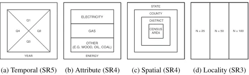
[image:5.612.49.292.48.122.2](d) Locality (SR3)
Fig. 5: Scale mosaic designs use containment and layout to reflect rela-tionships between scales – SRs in this context: e.g. seasons and yearly total (circular / hierarchical); types of and total household energy con-sumption (nominal / hierarchical); statistical boundaries (hierarchical) and ordered number of neighbors in locality (ordinal).
across the framework are likely to be important [23] in allowing ana-lysts to manage the complexities and volumes of data.
3.2 Possible Visual Designs
The possibilities for visually encoding the parameters framed through this structure are vast. Viable encodings can draw upon existing id-ioms, and in places the framework suggests that more novelty is re-quired. We investigate visual design options through our experience of dealing with geographic data (e.g. [41, 43, 46]), discussions with those using multivariate geographic data in their analysis [13, 15] and relevant literature on variable space observations (e.g. [45, 51]), local variations in multivariate comparison (e.g. [32]) and variable/feature selection (e.g. [25, 29, 39]). In Fig. 4 we present a collection of pos-sible visual design options for each cell of the framework, chosen to encourage fluid movement between cells. We separate visual
repre-sentations to emphasize the statistical and spatial (italicized)
relation-ships in each case. Visualizing many variables at theMicrolevel (
Mi-croMany) is deemed to be near impossible in many cases due to the volume of data – remembering that the thresholds between these con-ceptual states of affairs are defined to an extent by what is feasible in
a given context – while three proposals are expressed for the
Macro-ManyandMicroMultisituations. We investigate the use of correlation
matrices for variable comparison, especially for theMcases –Macro
-Micro/Multi-Many. Their compact nature often provides space into which alternative local statistics computed with different parameters can be visually represented in novel ways for comparison [14]. One
novel example is the scale mosaic, designed for the comparison of
global values for temporal-, attribute- or spatial-based SR or SE, or variations in locality definition. In Fig. 5 we split the correlation ma-trix cell using juxtaposition or containment [14]. Candidate designs reflect the variation in the data, with cyclical, linear and hierarchical arrangements shown. Frameworks for configuring hierarchical layouts may be usefully applied here [41]. Arranging cells in juxtaposition enables the number of variables that are under comparison to be
in-creased fromGlobalBi(e.g. Figs. 5, 8a) toGlobalMulti(Figs. 1b, 8b).
AsVincreases toGlobalManythe limited visual space requires a
sin-gle statistic be presented through color encoding. The variance, rank or the range of the values associated (e.g. Fig. 8c) are good candidates.
3.3 Geo-visual Parameter Space Analysis (gvPSA)
Given the fact that we treat the effects of geography, scale and
local-ity asparameterswithin multivariate geographical data analysis, our
framework can be characterized in terms of the established vPSA [38] model. vPSA is defined over three components: data flow model,
nav-igation strategies, and analysis tasks. In terms of thedata flow model,
we introduce geographical location and scale as inputs to any multi-variate analysis algorithm, with geodemographic classification the pri-mary focus of our work (Section 4). A second component of the data
flow model is thederived outputs. Our current focus is on variable
se-lection, with correlation and skewness coefficients computed and
vi-sualized asderived output. Due to the focus on simulation in vPSA
our overlap in terms ofnavigation strategiesis small but the
frame-work offers a structure to transition fromlocal-to-globalor
global-to-local, which we demonstrate through a prototype (Section 5).
Addi-tionally, our approach considers aninformed trial and error process
– to support variable selection in our geodemographic context. Here
we engage in some tasks described in vPSA. The first of these is
opti-mization, where we support analysts in finding a suitable subset of the variables by taking geography and scale into account through well-informed, robust decisions in variable selection. The second relates
to thesensitivityof the observations. We support this task by
includ-ing visual designs that inform on the scale and location dependency of multivariate relationships. Considering geography, scale and lo-cality as introduced in the previous section and the overlap with vPSA enables us to introduce our work as Geo-visual Parameter Space Anal-ysis (gvPSA).
4 APPLIEDCONTEXT: ENERGYGEODEMOGRAPHICS
The framework is inspired by and demonstrated in the context of our ongoing work in variable selection for energy geodemographics [16].
Geodemographic approaches classify areas through clustering
based on measured characteristics of thecharacteristics of the
resi-dent population[21]. Geodemographics are widely used for inferring characteristics about neighbourhoods, linking other relevant data, and making marketing and service delivery decisions. They are appropri-ate for energy consumer profiling in the UK as domestic energy con-sumption varies with geographic location [8] and is shown to correlate with many socio-economic characteristics of the population [8, 31]. Each area is allocated to the statistical cluster that best describes it. Membership can be mapped [42, 48] and used in modeling [21], with the uncertainties associated with the classification process explored through interactive graphics [43].
Generating a geodemographic classification is time-intensive and complex [21, 49]. The methodology used in the open-geodemographic classification developed by the UK Office of National Statistics (ONS) is well documented – the original Output Area Classification (OAC) used data from the 2001 UK Census [49] with amended variables and methodology for the second release for the 2011 Census [13].
4.1 Variable Selection: OAC Process
Suitable variables are selected for clustering from a pool of candidates, e.g. 167 variables were considered for OAC 2011 and reduced to 60 for the final classification [13]. Possible candidate variables for OAC 2001 and 2011 were initially identified based on a standard source SE and SR (Stage 1 of Fig. 6). Only variables representing all of the UK’s
SE were considered at the Output Areas (OA)2SR – hence ‘OAC’.
Standardization (stage 2 of Fig. 6) ensures all variables are at the same scale for comparison and clustering [21]. Once standardized, global statistics – for example the correlation coefficients – are used to assess variable suitability for the classification [13, 50]. Variable selection decisions are made based on variable distribution and mul-tivariate relationships as heavily skewed and strongly correlated vari-ables can bias the classification results [21]. Multiple varivari-ables are compared to assess their correlation, skewness and similarities. Vari-ables with little or no geographical variation also have little impact in producing geographically discriminating profiles [49]. As comparing the geographical variation of multivariate data is such a difficult task, the geographical variation is currently only explored as a final check when deciding whether to retain one variable over another [13, 49].
4.2 Variable Selection: Scale, Tasks & vPSA
The priorities and methods that guide domain specific and local clas-sification differ depending on the use-case. The effects of scale and geography on the variables under consideration are important factors throughout the process as documented in the literature [40, 50] and il-lustrated in Section 2. Our reading of the literature (e.g. [13, 21, 33, 40, 49, 50]), experience of geographical analysis and initial explorations of the effects of geography and scale on multivariate correlation lead
us to suggest: 1)four stagesof the variable selection process where
scale (SE and SR) decisions are made and may have an effect (Fig. 6); 2)five analytical tasksrelating to correlation, geography and scale that
can support geodemographic variable selection. Geodemographic
an-alysts confirm a need to be able to determinewhether and where[12]:
T1 variables correlate or are heavily skewed;
T2 local correlation or skewness differ from global values;
T3 globally correlating variables show geographical differentiation; T4 global correlation or skewness are sensitive to changes in SR; T5 variables are effected by the determination of locality.
Introducing local statistics3(as represented by the ‘Locality’ stage
of Fig. 6) asparametersto the process enhances variable selection
by exposing geographic variation and parameter sensitivities associ-ated with the variables. In vPSA [38] terms, the variable values and summary statistics from the standardize and locality stages of our pro-cess form the output values for our multivariate (variable selection) analysis (stage 4 of Fig. 6). The different options available at both stages, relating both to the resolution and extent considerations, form theparameterspace that, as in vPSA, affects the results of the analy-sis. We use our framework to guide the design of graphics for our soft-ware prototype, which shows correlations between multiple variables and their variation across scale and geography. Pathways through the framework guide the interactions through which the variable selection process is graphically augmented. We investigate the benefit of these methods informally in light of our work in multivariate geographical analysis through visual exploration.
4.3 Demonstrative Dataset
To demonstrate the process we use the 71 unique variables from the 2011 UK Census [34] that generate discriminating profiles at the na-tional level in OAC (41 were used in OAC 2001 [49] and 60 in OAC 2011 [35]). We augment these for energy geodemographics with a further 7 energy-related variables. Gas consumption, electricity con-sumption and fuel poverty levels come from the UK Department of Energy and Climate Change (DECC) [5, 6] and the 2011 UK Cen-sus [34] provides the further 4 variables on usage of the different cen-tral heating types: electric, gas, other (e.g. wood, coal or oil) or none.
In terms of scale, each variable from the Census is available at an
OA SR, whilst DECC variables are available at LSOA 20014. Both of
these Census units are not only relatively small in area but are specif-ically designed to produce an optimal arrangement in terms of social homogeneity, thereby reducing the impact of MAUP [28]. In terms of SE, the Census 2011 and consumption data are available for
Eng-land and Wales5and the fuel poverty indicator for England only. This
leads us to investigate multiple levels of spatial SR for the dataset of 78 variables, with SE fixed and focusing on England.
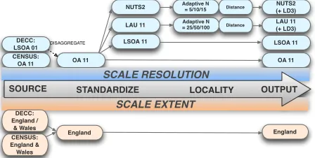
The source data scales are illustrated in Fig. 7, which uses the model shown in Fig. 6. Here, we show that values for the LSOA 2001 data are first disaggregated to OA 2011 units (171,372) for England, before being aggregated to three common levels of SR (see Fig. 7). These levels are: LSOA 2011 (32,844 units), LAU (326) and NUTS2 (32)
from theNomenclature of Territorial Units for Statistics[36].
In terms of localities, local summaries were calculated for NUTS2 and LAU using the adaptive moving window approach for three
dif-fering values ofN(see Fig. 7). LSOA and OA were too numerous
to perform the calculations given the computing resources available. The output scale (Fig. 7) that is available for representation in the final prototype provides four data sets – forming a geographical hierarchy. Each contains data for the 78 variables and are summarized as global statistics allowing the four SR to be compared globally, while NUTS2 and LAU offer additional local statistics and the opportunity to inves-tigate the sensitivity of locality, through varying the value of N.
4.4 Geodemographics and the Framework
In reference to our framework, current practice for geodemographic
variable selection [13, 21, 49] takes place in the first row Global,
where variable structure and relationships are compared from V =
3We use Pearson’s r Correlation Coefficient and Skewness because
spatially-weighted versions of these exists in theGWModel[27] R package.
4Second tier census boundaries aggregated from OA
5The Census 2011 has since been released for the whole of the UK
SCALE EXTENT SCALE RESOLUTION
SOURCE STANDARDIZE LOCALITY OUTPUT
TYPE
Source
Source Output
Output Aggregate
Filter Filter
WEIGHTING Moving Window Fixed/Adaptive Partitioning
Ir/regular Equal
[image:6.612.335.548.48.136.2]Distance
Fig. 6: Adding locality into the variable preparation process for selec-tion for geodemographic classificaselec-tion. Each stage – source, standard-ize, locality and output – involves both dimensions of SR and SE.
SCALE EXTENT
SCALE RESOLUTION
SOURCE STANDARDIZE LOCALITY OUTPUT
England DECC:
England / & Wales CENSUS: England &
Wales
England DECC:
LSOA 01
OA 11 CENSUS:
OA 11
DISAGGREGATE
LAU 11
NUTS2 Adaptive N = 5/10/15 Distance
Adaptive N = 25/50/100 Distance
LSOA 11 NUTS2 (+ LD3) LAU 11 (+ LD3) LSOA 11
OA 11
Fig. 7: The data scale resolution and locality definition (LD) options associated with the demonstrative dataset.
Unithrough toV =Many– 167 variables in the case of OAC 2011
[13]. The introduction of locality into the process (Figs. 6 and 7)
al-lows us to augment this analysis by exploring theMacroandMicro
rows through which we can investigate geographical variation. From our demonstrative data set (Section 4.3) the four levels of SR
pro-vide the ability to vary scale at theGlobal level of the framework,
through which the geographic variation of a single variable is con-sidered. Additionally the local statistics calculated at two SRs (with
32 and 326 values) can be associated with theMacroandMicro
lev-els of the framework. Graphical techniques for producing data dense
relational graphics [44] associated with the combinations ofVandL
across the framework are required to enable us to explore the effects of varying both scale and geography in our analysis.
5 PROTOTYPEVISUALDESIGN
We instantiated the framework in prototype software [24] by imple-menting the visual design options shown in bold in Fig. 4. These are
described here and in the accompanying video6.
5.1 Prototype Layout
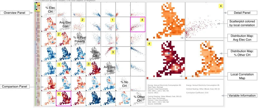
The prototype features three panels: overview, comparison and
de-tail (see Fig. 9). Theoverview panel allows all 78 variables to be
ranked by four global measures describing complimentary character-istics: theme (variable category), skewness (as an indication of dis-tribution), variance of correlation (as an indication of how correlation varies across all variables) and Moran’s I (to establish geographical
dependencies [2]). Thecomparisonpanel is an adaptable correlation
matrix (Fig. 1a-1c) suitable forMulti-to-Manyvariables. Rows and
columns represent variables ordered according to the overview panel. Each cell thus represents a pair of variables other than those on the diagonal, which relate to a single variable.
Cells in the matrix show pairwise correlation statistically and ge-ographically (Section 5.2) through scatterplots and maps colored by global or local correlation. This view adapts to color encoded cells or line glyphs (representing the scatterplot shape as a diagonal line) as the
number of variables increase fromMultitoMany. The central diagonal
[image:6.612.330.554.189.302.2](a) GlobalBi (b) GlobalMulti (c) GlobalMany
Fig. 8: Spatial scale mosaic with superimposed color encoded global
correlation coefficients for SR4:(a) V=Biand(a) V=Multi.(c)For
V=Manythe variance of the four correlation values is encoded – the
darker the more variation across SR for the variable pair.
shows the distribution of the variable in the row/column through inter-changeable views depending on the size of the matrix: histograms, variable distribution maps, local skewness maps or cell color encoded by global skewness from positive (purple) to negative (green). We use diverging and sequential ColorBrewer schemes [22] consistently
to show different forms of variation: e.g.RdBufor correlation (+1 red
to -1 blue),PrGnfor skewness andYlOrBrfor geographic distribution.
Alternative ColorBrewer schemes are used for the global measures in the overview panel.
Thedetailpanel represents theBiandUnicolumns of the frame-work, where the structure and pairwise correlation of any pair of vari-ables selected from the other panels are displayed (see Example 4 in Fig. 9). This consists of enlarged and enhanced views from the cor-relation matrix including: maps showing the geographical distribution of the individual variable or the local skewness, and pairwise local correlation, as well as a scatterplot presenting the local correlation.
In using different screen real estate to show relationships between
different numbers of variables (V) and local statistics (L) the three
panels populate distinct cells in the framework under contrasting con-straints.
5.2 Concurrent Geographical and Statistical Views
To represent the local values we use an asymmetrical matrixin the
comparison panel. Concurrent and complimentary views of local vari-ation draw upon the statistical and geographical design spaces above and below the diagonal respectively (Fig. 1c, Fig. 9). For these views inMacroManyandMicroMultiwe use different reduction techniques. For the maps in the matrix we aggregate the data spatially on the fly and present the average value as a colored square. We chose not to aggregate the statistical space but allow linked views in the detail panel to enable the aggregated geographical space to be explored in the non-aggregated statistical space. As our main focus is with LAU
and NUTS2 we can present the data forMultivariables in this way.
Some of the local relationships evident in the scatterplots require res-olution to establish the good continuation through which trends can be
detected (e.g. Fig. 9, scatterplot 1). As we move further into theMicro
space (e.g. the use of LSOA in this example) statistical aggregation is likely to be necessary.
5.3 Spatial Scale Mosaics
We use our scale mosaic design to present multiple spatial scale (SR4)
in our comparison and detail panels forGlobalBi(Fig. 8a) and
Global-Multi(Fig. 8b). Global correlation is shown in the matrix with global skewness filling the central diagonal. As our spatial SR is hierarchi-cal we use containment to reflect the shierarchi-cale relationships where space
allows. As we move toGlobalManythe number of pixels available
within each cell decreases and the ability to visually detect the dif-ferences between the scales reduces. We therefore revert to a single global summary (Fig. 8c). We use variance here as we are predomi-nantly interested in discovering whether a variable is scale dependent and by how much (alternatives in Section 6.2.2). Interaction between the three panels of the prototype allows for the detailed investigation
of the variation associated with the four SR in our data set. Clear ef-fects are identifiable for many variables, as discussed in Section 6.2.2 and shown in the accompanying video.
5.4 Navigating the Framework
An important aspect of the framework is that the visual representations adapt as we shift between the framework cells. In developing our
pro-totype we have implemented transitions in which bothLandVvary,
paying particular attention to transitions between some of the more
challenging cells: inL=MacrofromMulti-Many; inV=Manyfrom
Macro-Global; inV=BiandMultifromMacro-Micro. These
transi-tions are shown by arrows 1-3 in Fig. 4. The transition from
Macro-Multito MacroMany(Transition 1 in Fig. 4) occurs through spatial aggregation and over-plotting, which gradually reduces the amount of local detail shown on the screen. When the screen space becomes too
limited to showMacro, the visual representation shifts from
Macro-Many to GlobalMany(Transition 2) and the cell is color encoded.
Transition 3 fromMicro-Macrois shown in both theBi(detail panel)
and Multi(comparison panel) views by varying the number of cells
used to create the maps. These interactive and dynamic features show-ing framework in action are demonstrated in the supplementary video.
6 VARIABLEEXPLORATION ANDSENSITIVITYANALYSIS
The prototoype provides us with the capability to compare, select and filter variables, reorder the matrix according to key (global) features, automatically highlight strongly correlated or skewed variables, and focus on the details of selected variable pairs through linked larger vi-suals provided in the detail panel. This enables us to explore
geograph-ical variations in energy and OAC variables (T1-T3from Section 4.1)
as well as their sensitivities to scale and geography (T4-T5). The
sen-sitivities associated with geography, scale and locality can be explored
by varying the SR and the number ofNin the locality calculation. The
alternative local summary statistics that result can be depicted visually – perhaps as scale mosaics (see Fig. 5d) within maps or as graphics in juxtaposition as used in our exploration (see Fig. 10).
Values of N,L,V and level of SR can be varied interactively in
our prototype with visual depictions updating appropriately. The rapid interactive filtering, reordering and parameter variation supported by
the prototype allow us to engage in exploration throughinformed trial
and errorthat supports gvPSA.
6.1 Energy Variable Exploration
For example, visual exploration of global and local correlation and skewness reveals the energy variables to be highly geographical and
sensitive to changes in SR (T3, T5). As the SR increases from fine
(OA) to coarser resolution (NUTS2) the magnitude of global correla-tion increases, with extreme values more evident at the larger SRs. We explore the benefit of adding locality to our interpretation of correla-tion by discussing the local variacorrela-tion evident in the energy and other related variables through use of the prototype.
We consider aMacroMulticase in Fig. 9, with local correlation for
the data at LAU SR for each of the seven energy variables. Four
num-bered variable pairs of particular interest. Example 1 relates ‘
elec-tricity consumption’ and ‘gas consumption’, showing both strongly positive and strongly negative local correlations (as discussed in Sec-tion 2.2.2 and Fig. 3). Scatterplot 1 suggests two relaSec-tionships amongst LAUs, with map 1 showing the positive correlation to be characteris-tic of London and the North West and negative correlations elsewhere.
Example 2 (‘electricity consumption’ and ‘% in fuel poverty’) has a
near zero (0.03) global correlation coefficient, yet the local correlation varies substantially across England. Strong positive and negative local
correlations occur (e.g.>0.8 in the far South West,<-0.5 in the North
West). Alternatively Examples 3 and 4 show variable pairs with very
strong positive global correlation (T1), with the local correlation map
and scatterplots showing strength of positive correlation to vary locally
(T2). Both Example 3 (‘gas consumption’ and ‘gas central heating’)
and Example 4 (‘electricity consumption’ and ‘other central heating’)
% Elec CH
% Gas CH
% Other CH % No
CH % in Fuel
Poverty Avg Elec
Con
Avg Gas Con
1
1 2
2
3
3
4
4
4
4
Distribution Map: Avg Elec Con
Distribution Map: % Other CH
Local Correlation Map Scatterplot colored by local correlation
Variable Information Detail Panel
[image:8.612.95.527.51.232.2]Comparison Panel Overview Panel
Fig. 9: Software prototype showing all three panels andMicroMultiinformation in an asymmetrical matrix. Seven energy – consumption (Con),
fuel poverty and central heating (CH) – variables displaying locality information, based on an adaptive moving window with 25 neighbors
(N=25). Pairwise correlation examples 1-4 are highlighted and discussed in the text.
helpful in identifying key variables that differentiate populations and
behaviors despite global correlation. For instance, in Example 4 ‘
elec-tricity consumption’ and ‘other central heating’ correlate at the
na-tional scale (Global) and so one variable could be considered
redun-dant if geography is not considered. Our maps however show that this pair of variables allows us to discriminate between characteristics in the North West and South East that would not be captured if one of the
variables were omitted from analysis (T3).
When expanding the comparison to the non-energy variables and
skewness, local differences are also evident (T2). This is particularly
the case with gas consumption and central heating as the availability of gas is so geographically variant in the UK. Variables that are heavily skewed at the global level are often only extremely skewed in certain
locations (T3). For example ‘electric central heating’ has a global
skewness value of 4.3 yet the local skewness map shows extreme val-ues to be mainly located around London with some rural areas having
a negative skew (T2,T3). As the resolution oflocalityis enlarged (by
increasingN) the local patterns disappear and the skewness of
Lon-don dominates the global statistic. Local skewness evident in other variables frequently reveals a different skewness in densely populated urban areas such as London and the North West of England than the
rural areas particularly whereNis low. This effect reduces as the
num-ber of neighbors (N) increases and the values converge to the mean of
the full geographic extent (SE). The prototype shows where these
dif-ferences occur in multiple variables concurrently (T1,T2,T3). This
information can help to identify which variables differentiate which
localities (T3) and which variables are affected by SR (T4) as well as
changes in SE. Whilst SE is not accommodated in the software proto-type we can make some inferences – examples with strong correlation or heavy skewness in London for instance may be useful for a nation-wide profile but might not be suitable for a London (SE) based profile.
6.2 Geo-Visual Parameter Sensitivity Analysis
Having explored some of the ways in which correlations vary with scale and geography we next use the prototype to explore the sensitiv-ities associated with definitions of locality when varying the number
of neighbors (N) (T5) and when changing the SR (T4) at which global
statistics are calculated.
6.2.1 Varying Neighbourhood Parameterization (N)
In order to see which variables are most affected by varying the value
ofN(25, 50 and 100), we subdivide the cells of the comparison panel
and display the resulting graphics for each value ofNin juxtaposition.
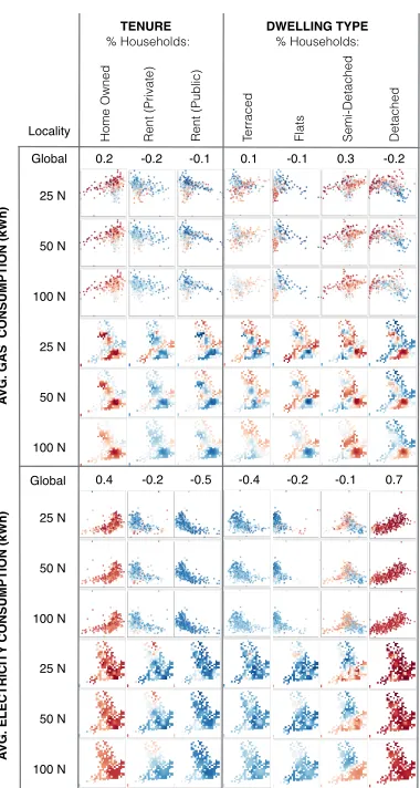
A small section of the matrix that results is shown in Fig. 10, with ver-tical juxtaposition in this instance. The full figure with more variables
and showing local skewness is supplied as supplementary material. In Fig. 10 geographical variation in local correlation between household variables and electricity or gas consumption is shown. In all examples we can see differences, particularly in the map view, as
the locality definition varies byN(T5). These differences depend on
the type of correlation pattern. When displayed in this manner and in-terpreted with a little local knowledge we can detect three types of
ge-ographical correlation pattern (T3): those that have largely urban/rural
correlations (e.g. ‘gas consumption’ and ‘home owned’), those
re-vealing little difference across the country (e.g. ‘electricity
consump-tion’ and ‘home owned’) and those with a distinctive North-South
di-vide (e.g. ‘electricity consumption’ and ‘semi-detached housing’ or
‘private-rented housing’). In Fig. 10 the correlation with gas largely shows an urban/rural trend; however, the other patterns are present in
the full supplementary figure – for example ‘gas’ and ‘no central
heat-ing’ shows a largely North-South divide, perhaps reflecting cultural
differences that may be important in energy geodemographics (T3).
In Fig. 10 there is also a clear difference between patterns of gas and
of electricity correlation when comparing local and global values (T2,
T3). Globally, gas is shown to not correlate with the other variables in
Fig. 10 as the values are near zero– the shapes of the scatterplots and the values reveal this. However, all examples show clear geographi-cal differences with most returning both highly negative and positive
correlations locally (T2). Visualizing data in this manner enables us to
relate local knowledge to the scale and locality dependent information and should result in more informed decision-making. Global
correla-tions with ‘electricity consumption’ are more varied; The two variables
with the weakest global correlations show clear and different local
pat-terns (‘rent private’ and ‘semi-detached’), whilst ‘detached’ has a very
strong global correlation and shows little variation locally (T3).
Ex-panding this analysis to other variables (see supplementary material) enables us to visually demonstrate that local statistical summaries are
not only dependant on the value ofNbut also heavily influenced by the
structure of the variables themselves – in terms of both their statisti-cal and geographistatisti-cal distribution. Variables with distinct geographistatisti-cal patterns, such as gas consumption, show greater variation in their cor-relations when explored at the local level but these vary depending on the comparator. Heavily skewed variables also have more local skew-ness variability than those that are more normally distributed.
These observations lead to a more robust understanding of the en-ergy variables through the investigation of correlation relations.
Fur-ther development is required to extend this analysis of varyingNto
sensitivi-25 N
50 N
100 N
A
VG
.
G
A
S
C
O
N
SU
MPT
IO
N
(k
W
h
)
A
VG
.
EL
EC
T
R
IC
IT
Y
C
O
N
SU
MPT
IO
N
(k
W
h
)
Home Owned Rent (Private) Rent (Public) Terraced Flats Semi-Detached Detached
TENURE DWELLING TYPE
Locality
25 N
50 N
100 N
25 N
50 N
100 N
25 N
50 N
100 N
% Households: % Households:
Global 0.2 -0.2 -0.1 0.1 -0.1 0.3 -0.2
[image:9.612.76.266.44.400.2]0.4 -0.2 -0.5 -0.4 -0.2 -0.1 0.7 Global
Fig. 10: A selection of household related variables in comparison with
gas and electricity consumption when number of neighbors (N) in the
locality is varied (25, 50 and 100) for LAU. Dark red shows positive correlation and dark blue represents negative correlation in statistical (top) and geographic (bottom) views for each variable pair.
ties associated with the definition of locality across multiple variables. The framework identifies and relates parameters for gvPSA and views through which gvPSA tasks can be accomplished.
6.2.2 Varying Scale Resolution (SR)
Visual exploration of the effects of varying scale (T5) draws upon the
scale mosaic view in the prototype. We use it to represent global cor-relation at a number of scales. Five forms of sensitivity are identified in our multivariate data set, as shown in Fig. 11. Of the 78 variables in
the prototype, the majoritystrengthenwith scale with the global
cor-relation getting stronger as the SR increases from fine resolution (e.g. OA) to coarse (e.g. NUTS2). Pairs of variables that are associated with regional trends, and local variability, are likely to exhibit these charac-teristics. Examples include Fig. 11d, which shows how the correlation
between ‘gas central heating’ and ‘electricity consumption’
strength-ens in a negative sstrength-ense from -0.5 to -0.8 as the resolution increases. Constantshows variables in which correlation is scale invariant, an unusual pattern in our analysis of OAC variables that are either very similar or the direct inverse of each other. For example, Fig. 11a,
shows ‘Aged 65+’ from OAC 2001 with ‘Aged 65-89’ from OAC
20117. That the strong correlation is independent of scale suggests
limited discriminatory value here, unless geographic (regional)
differ-ences are encountered. Polarityrelates to change in the sign of the
correlation value, e.g. Fig. 11b shows a positive correlation between
7Further discrimination of age group variables were added to OAC 2011.
(a) Constant (b) Polarity (c) Fluctuates (d) Strengthens (e) Weakens
Fig. 11: Five forms of scale sensitivity as SR increases from fine reso-lution to generalized using the scale mosaic design. Color refers to the degree of positive (red) or negative (blue) correlation.
‘flats’ and ‘separated/divorced’ at OA, but a negative correlation at
NUTS2.Weakensoccurs rarely in our analysis, but Fig. 11e shows an
example where ‘average house size’ and ‘single status’ has a
corre-lation value of -0.8 at OA level and this decreases to -0.7 at NUTS2. Fluctuatesis particularly sensitive to increases in scale and levels of
correlation both strengthen andweaken as scale changes. Fig. 11c
shows ‘electricity consumption’ with ‘people who bicycle or walk to
work’, with correlation at LAU notably higher (0.7) than both NUTS2
(0.4) and LSOA (0.4).
In our prototype design we use variance to encode theGlobalMany
(SR4)view. Whilst it provides a useful metric of the dependency each variable pair has on scale, this single number summary is not sufficient to identify all of five types of scale sensitivity in Fig.11. For example, it is not possible to distinguish weakening and strengthening trends. Alternative global measures depending on the analysts’ interests and
foci, may be appropriate for theGlobalManyview. For example, rank
correlation or the maximal information coefficient may be more appro-priate for identifying monotonically increasing or decreasing relations. They are applicable summaries within our broad framework.
In general, the mosaics reveal that correlations at the SRs of OA and LSOA are less strong than those at the two coarser SRs of LAU and NUTS2. The parameters are likely to be sensitive to processes that operate at different scales – with differences within and between regions depending upon the scales and localities used, thus justifying the consideration of resolution and extent as parameters in gvPSA.
7 DISCUSSION
We provide a framework with candidate designs, interactions and guidance for comparing and making sense of geographic aspects of multiple variables. We reflect on this framework, prototype designs and the applied context of geodemographic variable selection.
7.1 Applied Context
Using variables with geographical variation helps produce more dis-criminating profiles when creating geodemographic classifiers [49]. The addition of the locality stage (see Fig. 6) in the variable selec-tion process helps determine geographic variability. Whilst this in-creases the complexity of the process, our framework offers guide-lines to allow many variables to be visualized concurrently with the consideration of local variation. The prototype shows how this might be achieved – exploration that unearths interesting patterns and funda-mental differences when visualizing local, rather than global statistics.
The fluid transition fromGlobaltoMacrotoMicroand the three panel
prototype layout design allow strongly correlated variables to be dis-covered at the global level and then investigated through exploration of their geographical variation at the local level.
[image:9.612.307.561.48.107.2]We continue to develop our design suggestions as we apply our framework to other application areas. We are currently working to im-prove the quality of future survey data by identifying geographic and demographic patterns in response rates. This involves a large number
of census and related variables to investigatemodel rates of response
to household surveys8. In this context both time and attribute-based SR and SE are important in addition to spatial scale. The appropriate and informed selection of a limited set of discriminating variables is an important process in this analysis and one that can be supported by the framework, techniques and prototype software.
7.2 Feedback
Demonstrating the prototype to the creator of OAC 2011 [12] resulted in a positive reaction to the framework and its implementation. Al-though the prototype design itself was considered too complex for current practice due to the sheer amount of new information being pre-sented, the approach was seen as relevant and visual designs regarded as being potentially useful.
The scale mosaic and local correlation matrices (Figs. 1b and 1c) were considered as a big improvement over current practices, though some may have been a little too data dense. We acknowledge that considering local statistics and the parameters of geography and scale increases the amount of information to which one must attend whilst working with multiple variables. However, our framework
accom-modates this with reductions inV and/orLand associated graphical
updates as required enabling users to manage the information being presented. These could be permanent or temporary, whilst the views and their meanings are learned. We cannot provide evidence that this learning will occur, but we can accommodate richer graphics that con-tain information deemed to be important should the need arise.
Even at the global level, the prototype interaction and reordering possibilities were seen as more useful than the static matrices used to select variables for OAC 2011. The scale mosaics and our compar-ison of four SR were considered useful for local or domain specific geodemographics, where particular data are likely to be available at different SR and SE. In reality, value of the framework be determined by the detail of its instantiation. This is highly likely to be depen-dent on characteristics of data, task, technology and user. It provides a structure through which use-case specific workflows may be generated to help users deal with large amounts of information. It is sufficiently flexible to accommodate many of these in a range of contexts.
7.3 Limitations
A number of limitations from a user-perspective were identified in Section 7.2. Here, we reflect on some other limitations.
Ourframework is general, partially populated and contains only
broad design guidelines.Specific designsare untested and only
evalu-ated internally though our ongoing work in this domain. We employed a correlation matrix as the predominant layout for comparison (e.g. in the comparison panel of the prototype), but whilst further design work would be needed to adapt these techniques to multiple scales, more space-efficient visualization techniques [30] could be used.
The nature of local statistics means that some summaries are based upon small samples, perhaps leading to instability. Some patterns de-tected (or missed) may be dependent on artefacts of the graphics – orderings of matrices, layering of scatterplots and visual aggregation (as in the case of the maps in the prototype). We have not accounted for these effects in the current designs.
Whilst theprototypeenables us to efficiently explore sensitivities in
SR and locality definition (T1–T5) it does not implement the
frame-work fully. For example, our consideration of the problem of alter-native locality definitions is incomplete, involving the results of just one approach. Local statistics were pre-calculated for NUTS2 and
LAU only with small numbers ofN. Statistics were not calculated at
the higher resolution LSOA and OA levels due to limited resources. It elicited feedback and demonstrated potential, but more work is needed to further study the effects of scale on multivariate correlation for more
8https://blogs.city.ac.uk/addresponse/
SRs, different SEs and different locality definitions; e.g. by combining the mosaic scale design within the map squares. As such, we are only able to address certain aspects of the vPSA model and apply them to geodemographics. We will need to make calculations more efficient to demonstrate the full effects of varying the parameters of the geodemo-graphic classification model in real time so that gvPSA can be under-taken on the modeling as well as on the variable selection task through informed trial and error.
These issues can be addressed through further design, development and experimentation. Initial findings suggest that such work will be worthwhile. Whilst we do not yet have usable software to make the visualization of multiple variables across scale and geography man-ageable in the manner that is our aim the prototype has enabled us to develop and evaluate approaches, identify effects and establish needs.
8 CONCLUSION ANDFURTHERWORK
Our framework for visualizing multivariate data across scale and ge-ography is the fundamental contribution of our research. It allows some of the sensitivities and complexities of multivariate geographic data to be investigated through visual means and provides a basis for structuring this activity. By instantiating key aspects of the framework in software, we offer design proposals and visualization techniques to support such work. In doing so we have applied known statistics,
geographically weighted statistics, newvisual designs(scale mosaics;
asymmetrical correlation matrices) that show correlation, scale and ge-ography, and interactions that established a new construct – gvPSA (geographical vPSA). The approach has supported tasks that we deem important in multivariate geographical analysis and enabled us to iden-tify notable local variations in geography and scale that were hidden by global statistics in our own geographic work. We demonstrate that these approaches have clear application through analytical exploration (Section 6) in which geographical variation and scale are shown to be important considerations in multivariate correlation.
Although we argue that these approaches are beneficial to the geodemographic variable selection process and have revealed vari-ables that are variously geographically correlated, further work is
needed to determine the exact effects that variables with a ‘weak global
and strong local’ or a ‘weak local and strong global’ correlation may
have on the final classification. Further work, where thedata flow
model[38] is realized in its entirety, with geodemographic
classifica-tions as theoutputand classifiers as themodelcould demonstrate how
the variable decisions informed by geography and scale affect the
clas-sifier, increasing the need for effective gvPSAnavigation strategies.
We would like to see the framework populated with further effective encodings that achieve a usable balance between information density and pragmatism. We hope to develop pathways through it to support sophisticated multivariate geographical analysis. But the true value of the ideas implemented in the prototype will only be established through the addition of robust and effective functionality to support navigation, selection and sense-making in applied contexts. A sys-tem that applies the framework fully would allow analysts to record and select the various geographies that are distinguished through local analysis and their relationships with correlating variables. Whilst feed-back received from colleagues developing geodemographic classifiers showed the potential of the framework and prototype it also demon-strated the challenges associated with presenting the rich information associated with gvPSA and thus of implementing usable systems for this activity. Iterative user-centred approaches would be key in design-ing a system that built on the contributions presented here to allow in-teractive variable selection and geodemographic classification through which the effects of scale and geography on clustering outputs could be assessed in real time in their geographic contexts.
ACKNOWLEDGMENTS