Graph Orientation and Flows Over Time
?Ashwin Arulselvan1??, Martin Groß2, and Martin Skutella2
1
Department of Management Science, University of Strathclyde
2
Institut f¨ur Mathematik, TU Berlin, Str. des 17. Juni 136, 10623 Berlin, Germany
gross,[email protected]
Abstract. Flows over time are used to model many real-world logistic and routing problems. The networks underlying such problems – streets, tracks, etc. – are inherently undirected and directions are only imposed on them to reduce the danger of colliding vehicles and similar problems. Thus the question arises, what influence the orientation of the network has on the network flow over time problem that is being solved on the ori-ented network. In the literature, this is also referred to as thecontraflow orlane reversalproblem.
We introduce and analyze theprice of orientation: How much flow is lost in any orientation of the network if the time horizon remains fixed? We prove that there is always an orientation where we can still send 13 of the flow and this bound is tight. For the special case of networks with a single source or sink, this fraction is 1
2 which is again tight. We present more results of similar flavor and also show non-approximability results for finding the best orientation for single and multicommodity maximum flows over time.
1
Introduction
Robbins [19] studied the problem of orienting streets as early as 1939, motivated by the problem of controlling congestion by making streets of a city one-way during the weekend. He showed that a strongly connected digraph could be obtained by orienting the edges of an undirected graph if and only if it is 2-edge connected.
The problem of prescribing or changing the direction of road lanes is a strategy employed to mitigate congestion during an emergency situation or at rush hour. This is called acontraflowproblem (or sometimesreversible flow orlane reversal problem). Contraflows are an important tool for hurricane evacuation [24], and in that context the importance of modeling time has become prevalent in the past decade [25]. It is also employed to handle traffic during rush hours [10].
?Supported by the DFG Priority Program “Algorithms for Big Data” (SPP 1736)
and by the DFG Research CenterMatheon“Mathematics for key technologies” in Berlin. An extended abstract [1] has appeared in proceedings of the 25th Interna-tional Symposium on Algorithms and Computation (ISAAC ’14).
??
Flows over time(also referred to asdynamic flows) have been introduced by Ford and Fulkerson [7] and extend the classic notion of static network flows. They can model a time aspect and are therefore better suited to represent real-world phe-nomena such as traffic, production flows or evacuations. Ford and Fulkerson studied the maximum flow over time problem, and described an efficient algo-rithm to solve it. This problem consists of a given time window in which as much flow as possible is to be sent from a source to a sink. An application for this are traffic problems where a high throughput is important, e. g., where many people need to get to a destination in a fixed time window – for example, from suburbs into the city and vice versa during rush hours; see, e. g., [16].
For evacuations, quickest flows (over time) are the model of choice. They are based on the idea that a given number of individuals should leave a dangerous area as quickly as possible [4, 6]. Such an evacuation scenario is modeled by a network, with nodes representing locations. Nodes containing evacuees are denoted as sources while the network’s sinks model safe areas or exits. For networks with multiple sources and sinks, quickest flows are also referred to as quickest transshipments [13] and the problem of computing them is called an evacuation problem [21]. A strongly polynomial algorithm for the quickest flow problem was described in [12]. For a more extensive introduction to flows over time, see [20].
In this paper, we are interested in combining the orientation of a network with flows over time – we want to orient the network such that the orientation is as beneficial as possible for the flow over time problem. We will assume that we can orient edges in the beginning, and cannot change the orientation afterwards. The assumption is reasonable in an evacuation setting as altering the orientation in the middle of an evacuation process can be difficult or even infeasible, depending on the resources available. We also assume that each edge has to be routed completely in one direction – but this will not impose any restriction to our modeling abilities, as we can model lanes with parallel edges if we want to orient them individually.
based dynamic traffic assignment model, wherein they allowed reversal of partial capacities.
Our Contribution. In Section 3 we study theprice of orientationfor networks with single and multiple sources and sinks, i. e., we deal with the following ques-tions: How much flow is lost in any orientation of the network given a fixed time horizon? And how much longer do we need in any orientation to satisfy all supplies and demands, compared to the undirected network?
To our knowledge, the price of orientation has not been studied for flows over time so far. It follows from the work of Ford and Fulkerson [7] that for maximum
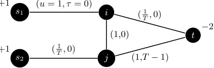
s-t-flows over time the price of orientation is 1: Ford and Fulkerson proved that a maximum flow over time can be obtained by temporally repeating a static min-cost flow and thus uses every edge in one direction only. The latter property no longer holds if there is more than one source or sink; see Fig. 1.
s2
+1 s1
+1
t −
2
j i (u= 1, τ = 0)
(1
T,0)
(1,0)
(1,T−1) (1
T,0)
Fig. 1. An instance with time horizon T where flow has to use edge {i, j} in both directions: At most T1 units of flow can reach the sink via path s2, j, t due to the capacity of edge{s2, j}and the transit time of edge{j, t}. Thus, a meaningful amount of flow from sources2 can only be sent via paths2, j, i, tand thus blocks edge{i, t}. As a consequence, flow originating at sources1 needs to take the paths1, i, j, t.
We are able to give tight bounds for the price of orientation with regard to the flow value, and we show that the price of orientation with regard to the time horizon cannot be smaller than linear in the number of nodes. Table 1 shows an overview of our results. Our main result is the tight bound of 3 on the flow price
Sources Sinks Flow Value Time
Price Reference Price Reference
1 1 1 Ford, Fulkerson [7] 1 Ford, Fulkerson [7]
2+ 1 2 Theorem 3 Ω(n) Theorem 4
1 2+ 2 Theorem 3 Ω(n) Theorem 4
[image:3.612.204.414.307.374.2]2+ 2+ 3 Theorem 1, 2 Ω(n) Theorem 4
Table 1.An overview of price of orientation results.
that is capable of simulating balances through capacities of auxiliary edges. This allows us to transform a problem with supplies and demands to the much simpler case of a single source with unbounded supply and a single sink with unbounded demand. We characterize the properties that the capacities of the auxiliary edges should have for a good approximation, and describe how they can be obtained using an iterative approach that uses Brouwer fixed-points. On the negative side, we give an instance whose price of orientation is not better than 3.
Since we have two ways to pay the price of orientation – decreasing the flow value or increasing the time horizon – the question arises whether it might be desirable to pay the price partly as flow value and partly as time horizon. We prove that by doing so, we can achieve a bicriteria-price of 2/2 for the case of multiple sources and sinks, i. e., we can send at least half the flow value in twice the amount of time.
In Section 4 we analyze the complexity of finding the best orientation to minimize the loss in time or flow value for a specific instance. We are able to show that these problems cannot be approximated with a factor better than 2, unlessP =N P. Furthermore, we extend this to two multicommodity versions of this problem and show that these become inapproximable, unlessP =N P.
2
Preliminaries
Networks and Orientations. Anundirected network over time N consists of an undirected graph G with a set of nodes V(G), a set of edges E(G), capacities
ue ≥ 0 and transit times τe ≥ 0 on all edges e ∈ E(G), balances bv on all nodesv∈V(G), and a time horizonT ≥0. For convenience, we defineV(N) :=
V(G), E(N) :=E(G). The capacityueis interpreted as the maximalinflow rate of edge eand flow entering an edgeewith a transit time ofτe at timeθ leaves
e at timeθ+τe. We extend the edge and node attributes to sets of edges and nodes by defining: u(E) := P
e∈Eue, τ(E) := Pe∈Eτe and b(V) :=Pv∈V bv. We denote the set of edges incident to a nodev byδ(v).
We defineS+:={v∈V(G)| b
v>0} as the set of nodes with positive balance (also calledsupply), which we will refer to assources. Likewise, we defineS−:= {v∈V(G)| bv<0}as the set of nodes with negative balance (calleddemand), which we will refer to as sinks. Additionally, we assume that P
v∈V(G)bv = 0 and defineB :=P
v∈S+bv. To define adirected network over time, replace the undirected graph with a directed one. In a directed network, we denote the set of edges leaving a nodev byδ+(v) and the set of edges entering vbyδ−(v) for
allv∈V(G).
Anorientation −→N of an undirected network over time N is a directed network over time −→N = (−→G ,−→u , b,−→τ , T), such that −→G, −→u and−→τ are orientations ofG,
u and τ, respectively. This means that for every edge {v, w} ∈ E(G) there is either (v, w) or (w, v) in E(−→G) (but not both) and (assuming (v, w)∈ E(−→G)) −
→u
(v,w) =u{v,w} and →−τ(v,w) =τ{v,w}. Recall that we can use parallel edges if
Flows over Time. A flow over time f in a directed network over time N = (G, u, b, τ, T) assigns a Lebesgue-integrable flow rate function fe : [0, T)→R+0 to every edgee∈E(G). We assume that no flow is left on the edges after the time horizon, i. e.,fe(θ) = 0 for allθ≥T−τe. The flow rate functionsfehave to obey capacity constraints, i. e.,fe(θ)≤uefor alle∈E, θ∈[0, T). Furthermore, they have to satisfy flow conservation constraints. For brevity, we define the excess of a node as the difference between the flow reaching the node and leaving it: exf(v, θ) := Pe∈δ−(v)
Rθ−τe
0 fe(ξ) dξ −
P
e∈δ+(v)
Rθ
0 fe(ξ) dξ. Additionally, we define ex(v) := ex(v, T). Then we can write the flow conservation constraints as
ex(v) = 0,ex(v, θ)≥0 for allv∈V(N)\(S+∪S−), θ∈[0, T),
0≥ex(v, θ)≥ −bv for allv∈S+, θ∈[0, T), 0≤ex(v, θ)≤ −bv for allv∈S−, θ∈[0, T). Thevalue |f|θ of a flow over timef until timeθ is the amount of flow that has reached the sinks until time θ: |f|θ :=P
s−∈S−exf(s−, θ) with θ ∈ [0, T]. For brevity, we define|f|:=|f|T.
We define flows over time in undirected networks over timeN by transforming
N into a directed networkN0, using the following construction. We replace every undirected edgee={v, w} ∈E(N) by introducing two additional nodesvw,vw0
and edges (v, vw), (w, vw), (vw, vw0), (vw0, v), (vw0, w). We set u(vw,vw0) =ue
andτ(vw,vw0)=τe, the rest of the new edges gets zero transit times and infinite capacities. This transformation replaces all undirected edges with directed edges, giving us the directed networkN0. Every flow unit that could have used{v, w} from either v to w or w tov must now use the new edge (vw, vw0), which has the same attributes as {v, w}. The other four edges just ensure that (vw, vw0) can be used by flow from v to w or w to v. Thus, whenever we consider flows over time in N, we interpret them as flows over time inN0 instead.
We will use edges with zero transit times and infinite capacity repeatedly from now on. Such edges can be traversed instantly and be used by as much flow as desired – thus, they can neither become bottlenecks nor do they affect the transit time of flow using them. They can be seen as an extreme case of very short streets with a very high number of lanes.
Maximum Flows over Time. Themaximum flow over time problemconsists of a directed or undirected network over timeN = (G, u, b, τ, T) where the objective is to find a flow over time of maximum value. The sources and sinks have usually unbounded supplies and demands in this setting but it can also be studied with finite supplies and demands. In the latter case, the problem is sometimes referred to astransshipment over timeproblem. If supplies and demands are unbounded, we usually introduce a super-source s (super-sink t) with an infinite capacity and zero transit time arc to all sources (from all sinks).
1. Compute a static s-t-flowxmaximizing
T|x| −X e∈E
xeτe.
with |x| being the flow value of x. The transit times only appear in the objective function as costs. Equivalent to this is adding an edge (t, s) with infinite capacity and cost −T to the network, followed by a minimum cost circulation computation in this extended network (transit times are again interpreted as costs).
2. Due to flow conservation, xcan be decomposed into flows along paths and cycles. This yields a flow decomposition (xP)P∈P∪C of x, with P being a
family ofs-t-paths andC being a family of cycles, such that
xe=
X
P∈P∪C:e∈P
xP.
Thus, (xP)P∈P∪C describes the same flow as x, but uses path- and
cycle-variables instead of edge-cycle-variables.
3. Output the s-t-flow over time that for each path P ∈ P repeatedly sends
xP flow units into the path as long as possible, i. e., during the time interval [0, T −τP), where τP :=Pe∈Pτe.
This type of flow is called temporally repeated, because flow is sent into each path at a constant rate for as long as the total transit time of the path allows. A temporally repeated flow has the nice property that edges are only used in one direction, as it is based on a static flow decomposition.
Themaximum contraflow over time problem is given by an undirected network over time N = (G, u, b, τ, T) and the objective is to find an orientation −→N of
N such that the value of a maximum flow over time in−→N is maximal over all possible orientations ofN.
Quickest Flows. The quickest flow problem or quickest transshipment problem is given by a directed or undirected network over time N = (G, u, b, τ) and the objective is to find the smallest time horizon T such that all supplies and demands can be fulfilled, i. e., a flow over time with valueBcan be sent. Hoppe and Tardos [12] gave a polynomial algorithm to solve this problem. However, an optimal solution to this problem might have to use an edge in both directions; see Fig. 1.
The quickest contraflow problem is given by an undirected network over time
N = (G, u, b, τ) and the objective is to find an orientation−→N ofN such that the time horizon of a quickest flow in−→N is minimal over all possible orientations of
N.
3
The Price of Orientation
between the value of a maximum flow over timefN in N and maximum of the values of maximum flows over timef−→
N in orientations − →
N ofN: |fN|/→− max
N orientationof N |f−→
N|.
Similarly, thetime price of orientationfor an undirected network over timeN = (G, u, b, τ) is the ratio between the minimal time horizon T(f→−
N) of a quickest flowf−→
N in an orientation − →
N ofN and the time horizonT(fN) of a quickest flow over timefN inN:
min
− →
N orientationof N
T(f−→
N)/T(fN).
3.1 Price in Terms of Flow Value
In this subsection, we will examine the flow price of orientation. We will see that orientation can cost us two thirds of the flow value in some instances, but not more.
Theorem 1. Let N = (G, u, b, τ, T) be an undirected network over time, in whichB units of flow can be sent within the time horizonT. Then there exists an orientation −→N of N in which at least B/3 units of flow can be sent within time horizon T.
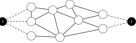
Proof. The idea of this proof is to simplify the instance, such that a temporally repeated solution can be found. Such a solution gives us an orientation that we can use, if the simplification does not cost us too much in terms of flow value. We will achieve this by simulating the balances using additional edges and capacities, creating a maximum flow over time problem which permits a temporally repeated solution. Then we show that the resulting maximum flow over time problem is close enough to the original problem for our claim to follow. Simulating the balances. We achieve this by adding a super source s and a super sinktto the network, resulting in an undirected network over timeN0= (G0, u0, τ0, s, t, T) withV(G0) :=V(G)∪ {s, t},E(G0) :=E(G)∪ {{s, s+}}|{s+∈
S+} ∪ { {s−, t} | s−∈S−},u0e:=uefore∈E(G) and∞otherwise,τe0 :=τefor
e∈E(G) and 0 otherwise. We refer to the newly introduced edges ofE(G0)\E(G) asauxiliary edges. Furthermore, we sometimes refer to an auxiliary edge by the unique terminal node it is adjacent to and write uv for ue, e = (s, v), fv for
fe, e = (s, v) and so on. An illustration of this construction can be found in Fig. 2.
The network N0 describes a maximum flow over time problem which has an optimal solution that is a temporally repeated flow, which uses each edge only in one direction during the whole time interval [0, T). Thus, there is an orientation −→
N0 such that the value of a maximum flow over time in N0 is the same as in −→
s t
Fig. 2.The modified network consisting of the original network (white), the superter-minals (black) and the dashed auxiliary edges.
Thus, we need to modifyN0such that balances ofNare respected – but without
using actual balances. This leaves us the option to modify the capacities of the auxiliary edges. In the next step, we will show that we can always find capacities that enforce that the balances constraints are satisfied and have nice properties for bounding the loss in flow value incurred by the capacity modification. These properties are then used in the last step to complete the proof.
Enforcing balances by capacities for auxiliary edges. In this step, we show that we can choose capacities for the auxiliary edges in such a way that there is a maximum flow over time in the resulting network that respects the original balances. Choosing finite capacities for some of the auxiliary edges will – in general – reduce the maximum flow value that can be sent, though. In order to bound this loss of flow later on, we need capacities with nice properties, that can always be found.
Lemma 1. There are capacities u00e that differ from u0e only for the auxiliary edges, such that the network N00 = (G0, u00, τ0, s, t, T)has a temporally repeated maximum flow over timef with the following properties
– the balances of the nodes in the original setting are respected: |fv|:=RT
0 fv(θ)dθ≤ |bv| ∀v∈S
+∪S−,
– and that terminals without tightly fulfilled balances have auxiliary edges with unbounded capacity:|fv|<|bv| ⇒uv=∞ ∀v∈S+∪S−.
Proof. The idea of this proof is to start with unbounded capacities and itera-tively modify the capacities based on the balance and amount of flow currently going through a node, until we have capacities satisfying our needs. In order to show that such capacities exist, we apply Brouwer’s fixed-point theorem on the modification function to show the existence of a fix point. By construction of the modification function, this implies the existence of the capacities.
Prerequisites for using Brouwer’s fixed point-theorem. We begin by definingU :=
P
v∈S+
P
of [0,∞). This will be necessary for applying Brouwer’s fixed point theorem later on.
Now assume that we have some capacities u ∈ [0, U]S+∪S− for the auxiliary edges. Since we leave the capacities for all other edges unchanged, we identify the capacities for the auxiliary edges with the capacities for all edges. Compute a maximum flow over timef(u) for (G0, u, τ0, s, t, T) by using Ford and Fulkersons’ reduction to a static minimum cost flow. For this proof, we need to ensure that small changes inuresult in small changes inf(u), i. e., we need continuity. Thus, we will now specify that we compute the minimum cost flow by using successive computations of shortest s-t-paths. In case there are multiple shortest paths in an iteration, we consider the shortest path graph, and choose a path in this graph by using a depth-first-search that uses the order of edges in the adjacency list of the graph as a tie-breaker. The path decomposition of the minimum cost flow deletes paths in the same way. This guarantees us that we choose paths consistently, leading to the continuity that we need.
Defining the modification function. In order to obtain capacities for a maximum flow over time that respects the balances, we define a functionh: [0, U]S+∪S− → [0, U]S+∪S− which will reduce the capacities of the auxiliary edges, if balances are not respected:
(h(u))v:= min
U, bv
|fv(u)|
uv
∀v∈S+∪S−.
|fv(u)|refers to the amount of flow going through the auxiliary edge of terminal
v ∈S+∪S− in this definition. If|fv(u)|= 0, we assume that the minimum is
U. Due to our rigid specification in the maximum flow computation,|fv(u)| is continuous, and thereforehis continuous as well.
Using Brouwer’s fixed-point theorem. Thus,his continuous over a convex, com-pact subset of RS+∪S−. By Brouwer’s fixed-point theorem it has a fixed point
u with h(u) = u, meaning that for every v ∈ S+ ∪S− either u
v = U or
uv = |fbv
v(u)|uv ⇔ bv =|fv(u)| holds, which is exactly what we require of our
capacities. ut
We can now choose capacities u00 in accordance to Lemma 1, and thereby gain
a maximum flow over time problem instanceN00 = (G0, u00, τ0, s, t, T), that has a temporally repeated optimal solution which does not violate the original bal-ances. What is left to do is to analyze by how much the values of optimal solutions forN andN00 are apart.
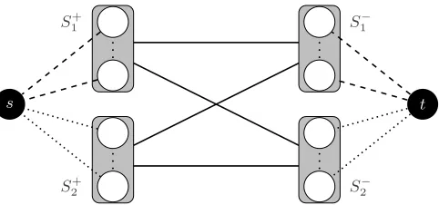
Bounding the difference in flow value betweenN andN00. We now want to show that we can send at least B/3 flow units in the networkN00 with the auxiliary capacities of the previous step. For the purpose of this analysis, we partition the sources and sinks as follows.
S1+:=
s+∈S+ us+ <∞ , S2+:=s+∈S+
us+=∞ , S1−:=
s−∈S− us−<∞ , S2−:=s−∈S−
s
. . . . . .
. . . . . .
t
S+ 1
S+ 2
S−1
[image:10.612.189.430.113.226.2]S−2
Fig. 3.The partitioning based on the capacities of the auxiliary edges. Dashed edges have finite capacity, dotted edges have infinite capacities.
The partitioning is also shown in Fig. 3.
Now letf be a temporally repeated maximum flow in N00 that does not violate balances. Notice that the auxiliary edges to terminals inS+2 andS2−, respectively, have infinite capacity and that the supply / demand of nodes in S1+ andS−1 is fully utilized. Thus,|f| ≥max
b(S+1), b(S1−) . Shouldb(S1+)≥B/3 orb(S1−)≥
B/3 hold, we would be done – so let us assume thatb(S1+)< B/3 andb(S1−)< B/3. It follows thatb(S2+)≥2/3B andb(S2−)≥2/3B must hold in this case. Now consider the networkN0with the terminals ofS+
1 andS
−
1 removed, leaving only the terminals ofS2+ andS2−. We call this networkN0(S+2, S2−). Let|f0| be the value of a maximum flow over time inN0(S2+, S2−). SinceB units of flow can be sent in N (and thereforeN0 as well), we must be able to send at leastB/3 units inN0(S2+, S2−). This is due to the fact thatb(S2+)≥2/3B, b(S2−)≥2/3B
– even ifB/3 of these supplies and demands were going toS1− and coming from
S1+, respectively, this leaves at least B/3 units that must be send from S2+ to
S2−. Thus, B/3≤ |f0|. Since the capacities of the auxiliary edges ofS2+ andS2−
are infinite, we can send theseB/3 flow units inN00as well, proving this part of the claim.
Thus, we have shown that a transshipment over time problem can be transformed into a maximum flow over time problem with auxiliary edges and capacities. If these edges and capacities fulfill the requirements of Lemma 1, we can transfer solutions for the maximum flow problem to the transshipment problem such that at least one third of the total supplies of the transshipment problem can be send in the flow problem. Finally, the proof of Lemma 1 shows that such capacities
do always exist, completing the proof. ut
s3
b= 1 s2
b= 1
v2
u= 1/T
v1
s1
b= 1
v4
τ= (1− δ)T u= 1
/T
v3
τ= T
t3 b=−1
t2 b=−1
τ= δT
t1 b=−1
[image:11.612.142.480.109.256.2]u= 1/T
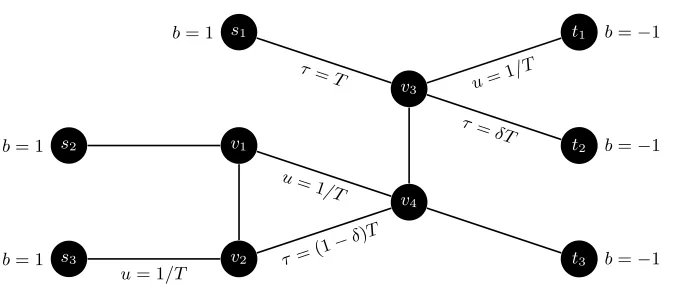
Fig. 4.An undirected network where every orientation can send at most one third of the flow possible in the undirected setting. Not specified transit times and balances are 0 and not specified capacities are infinite.
PPAD-completeness indicates that a problem is not FNP-complete [17]. How-ever, it is possible that the fixed-point can efficiently be found for the specific function we are interested in. One problem for finding such an algorithm is how-ever, that changing the capacity of one auxiliary edge does not only modify the amount of flow through its associated terminal but through other terminals as well – and this change in flow value can be an increase or decrease, making monotonicity arguments problematic.
Another potential approach could be to find a modification function for which (approximate) Brouwer fixed-points can be found efficiently. Using approximate Brouwer fixed-points would result in a weaker version of Lemma 1, where an additional error is introduced due to the approximation. This error can be made arbitrarily small by approximating the Brouwer fixed-point more closely, or by using alternative modification functions. However, finding a modification func-tion for which an approximafunc-tion of sufficient quality can be found efficiently remains an open question.
Now that we have an upper bound for the flow price of orientation and it turns out that this bound is tight.
Theorem 2. For any ε > 0, there are undirected networks over time N = (G, u, b, τ, T)in whichB units of flow can be sent, but at mostB/3 +εunits of flow can be sent in any orientation −→N of N.
Proof. In order to show this, we consider the network in Fig. 4 with three sources and sinks where each source has to send flow to a specific sink (due to capacities and transit times) but the network topology prevents flow from more than one source-sink pair being able to be send in any orientation.
have to orient {v3, v4} as (v3, v4) or lose the supply of s1 in the case of ε→0. Orienting{v3, v4}as (v3, v4) causes us to lose the demands oft1andt2, though, resulting in only one third of the flow being able to be sent.
Therefore let us now orient {v3, v4} as (v4, v3). Supply from s3 needs to go through{s3, v2}at a rate of at most 1/T. Thus, if we were to route flow through {s3, v2}and{v2, v4}we can send at most (T+ε−(1−δ)T)/T =ε/T+δtov4 (and the sinks) within the time horizon. Forδ, ε→0 this converges to 0 as well. Since we already lost the supply of s1, we need the supply of s3 if we want to send significantly more than one unit of flow. Therefore, we would have to orient {v1, v2} as (v1, v2) to accomplish this. However, due to the capacity of 1/T on {v1, v4}we can send at most 1 +δ/T flow through this edge, and one unit of this flow comes from s3, leaving only δ/T units for flow froms2. Thus, forδ, ε→0 the flow we can send converges to one.
In the undirected network, we can send all supplies. The supply froms1 is sent to t3, using{v3, v4} at time T. The supply froms2 is sent tot2, via{v1, v2} at time 0,{v2, v4} and{v4, v3} at time (1−δ)T. The supply froms3 is sent tot1 by{v2, v1},{v1, v4}and{v4, v3}during the time interval (0, T). This completes
the proof. ut
With these theorems, we have a tight bound for the flow price of orientation in networks with arbitrarily many sources and sinks. In the case of a single source and sink, we have a maximum flow over time problem and we can always find an orientation in which we can send as much flow as in the undirected network. This leaves the question about networks with either a single source or a single sink open. However, if we use the knowledge that only one source (or sink) exists in the analysis done in the proofs of Theorem 1 and Theorem 2, we achieve a tight factor of 2 in these cases.
Theorem 3. Let N = (G, u, b, τ, T) be an undirected network over time with a single source or sink, in which B units of flow can be sent within the time horizonT. Then there exists an orientation−→N ofN in which at leastB/2 units of flow can be sent within time horizon T, and there are undirected networks over time for which this bound is tight.
Proof. For this proof, we can use most of the argumentation of the proof of Theorem 1. The differences start only in the last part, where the differences in flow value between the original network N and the network with capacitated auxiliary edgesN00is considered. In the proof of Theorem 1, we partitioned the sources and sinks, but now we have either a single source or a single sink which does not need to be partitioned. Let us assume now that we have a single sink, the case with a single source follows analogously. We partition the sources as follows.
S1+:=
s+∈S+ us+<∞ , S2+:=s+∈S+
us+ =∞ ,
s
b= 1
v2
u= 1 /T
v1
v4
τ= (1−δ)T
v3
[image:13.612.205.416.114.198.2]u= 1/T
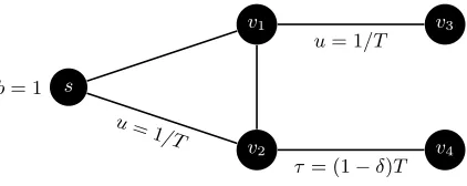
Fig. 5.An undirected network with a single source where every orientation can send at most one half of the flow possible in the undirected setting. Not specified transit times and balances are 0 and not specified capacities are infinite.
the sourcesS+1 removed and refer to the resulting network asN0(S2+, S−). Since
B units of flow can be sent inN (and thereforeN0 as well), we must be able to
send at leastb(S+2) units in N0(S+2, S−), since we still have all sinks available. Because of b(S2+)≥B/2, this proves the first part of the claim. For the second part, the lower bound, consider the construction from Theorem 2.
If we restrict the network described there tos2, s3, v1, v2, v4 and set the balance ofv4to−2, we can apply the same argumentation as in Theorem 2 to get a proof for the case of a single sink. For the case of a single source, we do something similar, but have to change something more. The result can be seen in Fig. 5;
the argumentation is analogous to Theorem 2. ut
3.2 Price in Terms of the Time Horizon
In this part, we examine by how much we need to extend the time horizon in order to send as much flow in an orientation as in the undirected network. It turns out that there are instances for which we have to increase the time horizon by a factor that is linear in the number of nodes. This is due to the fact that we have to send everything, which can force us to send some flow along very long detours – this is similar to what occurs in [9]. For this reason it is not a good idea to pay the price of orientation in time alone.
Theorem 4. There are undirected networks over time N = (G, u, b, τ, T + 1) with either a single source or a single sink in whichB units of flow can be sent within a time horizon of T, but it takes a time horizon of at least(n−1)/4·T
to send B units of flow in any orientation−→N ofN. This bound also holds ifG
is a tree with multiple sources and sinks.
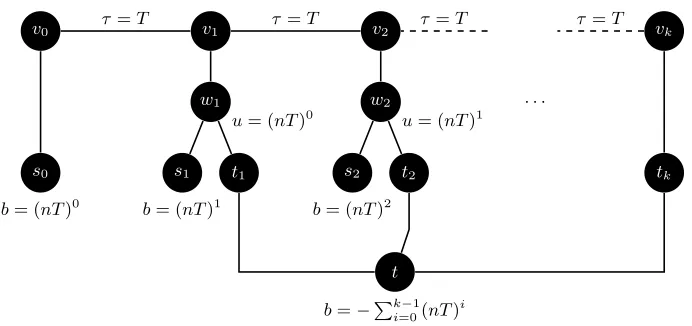
Proof. We define a family of undirected networks over timeNk by
V(Nk) :={s0, v0, vk, tk, t} ∪ {si, ti, vi, wi | i= 1, . . . , k−1},
E(Nk) :={{s0, v0},{vk−1, vk},{vk, tk},{tk, t}}
s0
b= (nT)0
v0 τ =T v1
w1
s1
b= (nT)1 t1
u= (nT)0
v2
τ=T
w2
s2
b= (nT)2 t2
u= (nT)1
τ =T
. . .
vk
τ =T
tk
t
b=−Pk−1
i=0(nT)
[image:14.612.138.484.113.276.2]i
Fig. 6. An undirected network with a single sink where every orientation requires a time horizon that is larger by a factor of at least (n−1)/4 compared to the undirected setting. Not specified transit times and balances are 0 and not specified capacities are infinite.
We define capacities, transit times and balances for this network by
ue:=
(
(nT)i−1 e={wi, ti} ∞ else , τe:=
(
T e={vi, vi−1}
0 else ,
bv :=
(nT)i v=si −Pk−1
i=0(nT)
i v=t
0 else
.
Fig. 6 depicts such a networkNk. It is possible to fulfill all supplies and demands in time T + 1 in the undirected network, if we route the supply of source si throughvi, vi+1, wi+1 and ti+1 to t. However, this requires using the{vi, wi} -edges in both directions. If we orient a {vi, wi} edge as (vi, wi), we can only route the supply of si viawi andti to t, which requires nT time units, due to the supply of si and the capacity of {wi, ti}. If we orient all {vi, wi} edges as (wi, vi), we have to route the supply froms0 viav0, v1, . . . , vkandtk tot, which requireskT time units. By construction of the network, we havek= (n−1)/4, which proves the claimed factor.
A similar construction can be employed in networks with a single source and multiple sinks (see Fig. 7). If we want to show the result for graphsGthat are trees, we can remove t and shift the demand to the nodes ti, i = 1, . . . , k and
give nodeti a demand of−(nT)i−1. ut
s0
v0 τ=T v1
w1
s1
u= (nT)k−2
t1
b=−(nT)k−1 v2
τ=T
w2
s2
u= (nT)k−3
t2
b=−(nT)k−2
τ =T
. . .
vk
τ =T
tk
b=−(nT)0
s
b=Pk−1
i=0(nT)
[image:15.612.137.479.113.276.2]i
Fig. 7.An undirected network with a single source where every orientation requires a time horizon that is larger by a factor of at least (n−1)/4 compared to the undirected setting. Not specified transit times and balances are 0 and not specified capacties are infinite.
s1
+1
t1
−1
s2
+1
t2
−1
s3
+1
tk−1
−1
sk
+1
tk
−1
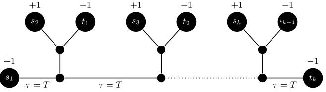
τ =T τ=T τ=T
Fig. 8. An undirected network with unit capacities where all supplies and demands can be fulfilled within a time horizon of T + 1. However, any orientation requires a time horizon of at leastkT+ 1. Not specified transit times and balances are 0.
we have to use the supply of a source si, 1< i≤k to fulfill the demand of sink
ti−1. This forces us to use the supply of s1 to fulfill the demand of tk, which takes at leastkT+ 1 time units.
3.3 Price in Terms of Flow and Time Horizon
[image:15.612.145.474.344.437.2]s t
Fig. 9.The modified network consisting of the original network (white) and the newly introduced nodes (black) and auxiliary edges (dashed).
Theorem 5. Let N = (G, u, b, τ, T) be an undirected network over time, in whichB units of flow can be sent within the time horizonT. Then there exists an orientation−→N ofN in which at leastB/2units of flow can be sent within time horizon 2T. The orientation and a transshipment over time with this property can be obtained in polynomial time.
Proof. In order to prove this claim, we will create a modified network with a larger time horizon in which we can send a temporally repeated flow which uses each edge in only one direction. This gives us then an orientation with the desired properties. Consider the networkN0 = (G0, u0, b0, τ0,2T) defined by
V(G0) :=V(G)∪ {s, t},
E(G0) :=E(G)∪ { {s, v} | bv>0} ∪ { {v, t} | bv<0},
u0e:=
bv
T e={s, v}
−bv
T e={v, t}
ue else
, τe0 :=
(
τe e∈E(G)
0 else ,
b0v :=
0 v∈V(G)
B v=s
−B v=t .
An illustration can be found in Fig. 9. We know that there is a transshipment over timef that sendsBflow units within timeT inN. We can decompose this transshipment into flow along a family of paths P with τP < T for all P ∈ P and interpret f as sending flow into paths P ∈ P at a rate offP(θ) at timeθ. Now consider a transshipment over time f0 that is defined by sending flow into the same paths as f, but at an averaged rate off0
P(θ) := 1 T
RT
0 fP(ξ) dξ for a pathP and a timeθ ∈[0, T). Since all paths P ∈ P have τP < T,f0 sends its flow within a time horizon of 2T. f0 sends B flow units as well, since we just averaged flow rates and the averaging guarantees that the capacities of the edges
e∈E(G0)\E(G) are not violated. We conclude that a maximum flow over time in N00:= (G0, u0, τ0, s, t,2T) has a value of at leastB.
over timef00 which uses each edge in only one direction. We can transformf00
into a transshipment over timef∗forNby cutting off the edges ofE(G0)\E(G). Due tou0{s,v}=bv/T,u0{v,t}=−bv/T and the time horizon of 2T, the resulting flow over time f∗ satisfies supplies and demands b00 with 0 ≤ b00v ≤ 2bv for
v∈V(G) withbv >0 and 0≥b00v ≥2bv forv∈V(G) withbv<0. Thus, 1/2f∗ sends at leastB/2 flow units in 2T time and uses each edge in only one direction without violating the balances b. Furthermore, this can be done in polynomial time, since the transformation and the Ford-Fulkerson algorithm are polynomial.
This concludes the proof. ut
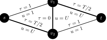
Earliest Arrival Flows. We now have tight bounds for the flow and time price of orientation for maximum or quickest flows over time. However, for application in evacuations, it would be nice if we could analyze the price of orientation for so-called earliest arrival flows as well, as they provide guarantees for flow being sent at all points in time. Unfortunately, we can create instances where not even approximate earliest arrival contraflows exist, because the trade-off between different orientations becomes too high.
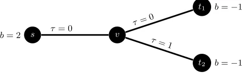
Earliest arrival flows are special quickest flows that maximize the number of flow units that have reached a sink at each point in time simultaneously. This is an objective that is very desirable in evacuation management, if the exact amount of available time is not clear in the planning stage. It is not clear that these flows exist in general, because they try to maximize multiple objectives at once – for each time point for which we try to maximize the flow value, we get an objective. Earliest arrival flows always exist if only one sink is present, as was first proven by Gale [8]. For multiple sinks, that is usually not the case if the sinks have a finite demand (see Figure 10), but approximations are still possible [2, 9].
s
b= 2 τ = 0 v
t1 b=−1
τ= 0
t2 b=−1
[image:17.612.186.429.465.539.2]τ= 1
Fig. 10.A directed network with sourcesand sinkst1, t2and unit capacities. Supplies and demands and transit times are as specified. Maximizing the flow value at time 1 requires fulfilling the demand oft1first. In this case, no flow arrives att2 before time 2. However, if we want to maximize the flow value at time 2, we fulfill the demand of
t2 first. In this case, no flow arrives at the sinks before time 1, but all demands are fulfilled by time 2 (whereas the first strategy only does so at time 3).
For every timeθ∈R+, letf∗
θ be a maximum flow over time with time horizon
pattern. An earliest arrival flow is a flow over time f which simultaneously satisfies|f|θ=p(θ) for all points in timeθ∈[0, T), respectively.
Anα-time-approximate earliest arrival flow is a flow over timef that achieves at every point in timeθ∈[0, T), respectively, at least as much flow value as possible at timeθ/α, i. e.,|f|θ ≥p θα
. Aβ-value-approximate earliest arrival flow is a flow over time f that achieves at every point in timeθ∈[0, T), respectively, at least a β-fraction of the maximum flow value at timeθ, i. e.,|f|θ≥ p(βθ). In practice, orienting road networks is an important aspect of evacuation man-agement. In terms of evacuations, earliest arrival flows (or approximations of them) are very desirable, as they provide optimal routings independently of the time that is available. The contraflow versions of these problems ask for an ori-entation−→N ofNand a flow over timef in−→N, such that|f|θ=p(θ),|f|θ≥p αθ
and|f|θ≥ p(βθ), respectively, for allθ. Notice thatprefers to the earliest arrival pattern of the undirected network in this case.
We are able to show that earliest arrival flows and the approximations developed in [2, 9] do not exist in this setting.
Theorem 6. There are undirected networks over timeN = (G, u, b, τ)for which an earliest arrival flow exists, but that do not allow for an earliest arrival con-traflow. This also holds for α-time- and β-value-approximative earliest arrival contraflows forα < T /2 andβ < U, whereT andU are the largest transit time and capacity in the network.
Proof. Consider the network depicted in Fig. 11. We can orient the edge{v1, v2}
s
v2
u= U τ=
T /2 v1
u= 1 τ= 1
u=U
τ= 0 t
u= 1 τ= 1
u= U τ=
[image:18.612.215.403.432.503.2]T /2
Fig. 11. An undirected network with sources and sink t and capacities and transit times as specified.
as (v2, v1) and have flow arriving with a rate ofU εstarting at time 2T. However, we have no flow arriving before timeT + 1 using this orientation. If we use the orientation (v1, v2) instead, we can have flow arrive at time 2, but at a rate of 1 instead of U. ForU T, this trade-off makes it impossible to find an earliest arrival contraflow.
using the orientation (v2, v1), we could have sent them by time 2T+ 1. Sending flow at a rate ofU using the orientation (v2, v1) results in no flow units being sent until time T + 1, but flow could have been sent as early as time 2 using the other orientation. This yields the non-approximability result for α -time-approximations.
Forβ-value-approximations, we need to use the orientation (v1, v2) to have some flow arrive starting at time 2. However, using the other orientation allows us to send flow at a rate ofU, yielding a ratio that converges to U, which concludes
the proof. ut
4
Complexity Results
Furthermore, we can show non-approximability results for several contraflow over time problems. More specifically, we can show that neither quickest con-traflows nor maximum concon-traflows over time can be approximated better than a factor of 2, unless P = N P. Maximum flows over time and quickest flows can also be defined for the case ofmultiple commodities. In this case we replace the supplies and demands b by supplies and demands bi for all commodities
i= 1, . . . , k. Each commodity has to fulfill its own flow conservation constraints, and supply from one commodity can only be used for the demands of the same commodity. However, the capacities of the network are shared by all commodi-ties. This generalization leads to maximum multicommodity (contra)flow over time,quickest muticommodity (contra)flow problems. In this setting it can also be interesting to maximize the minimal fraction of flow of each commodity to its total demand. This is referred to asconcurrent multicommodity (contra)flow over timeproblem. For multicommodity contraflows over time, we can even show that maximum multicommodity concurrent contraflows and quickest multicom-modity contraflows cannot be approximated at all, even with zero transit times, unlessP =N P.
Theorem 7. The quickest contraflow problem cannot be approximated better than a factor of2, unlessP =N P.
Proof. Rebennack et. al [18] showed the NP-hardness of this problem. The re-duction technique they provide can also be used to show a non-approximability claim, if we modify the transit times used in their reduction. We give a brief sketch of their reduction technique, which is based on the SAT problem. We construct an instance for the quickest contraflow problem from an instance for the 3-SAT problem with`clausesc1, . . . , c`overkvariablesx1, . . . , xkas follows.
1. For each clause ci, we create a source c+1 and a sinkc
−
1 with a supply and demand of 1 and -1, respectively.
2. For each variable xi, we create four nodes: x1i and x2i for its unnegated literal, and ¯x1
i, ¯x2i for its negated literal. These nodes get neither supplies nor demands. Furthermore, we create a sourcesiand a sinktiwith a supply and demand of 1, respectively. Finally, we create edges
x1 i, x2i ,
¯
si, x2i ,
si,x¯2i with a transit time of τ2 and edges
ti, x1i ,
ti,x¯1i with a transit time ofτ1.
3. For each clause ci = xi1 ∨xi2 ∨x¯i3 we create edges
c+i, x1i1 , c+i , x1i2 ,
c+i ,x¯1
i3 with a transit time ofτ1and edges
c−i , x2 i1 ,
c−i , x2 i2 ,
c−i ,x¯2 i3
with a transit time ofτ2.
All capacities are infinite. Fig. 12 depicts such a construction.
YES-Instance → Routable in time τ1+ 2τ2. We derive an orientation from an assignment for the SAT problem that fulfills all clauses. If variable xi is set to 1 in the assignment, we orient
x1
i, x2i as (x1i, x2i) and
¯
x1
i,¯x2i as (¯x2i,x¯1i). Otherwise, we orient
x1
i, x2i as (x2i, x1i) and
¯
x1
i,x¯2i as (¯x1i,x¯2i). All other edges are oriented away from the sources or towards the sinks, respectively. A clause source c+i with a fulfilled literal xi can send 1 flow unit along c+i →
x1i →x2i →c−i , and each variable source si can send 1 flow unit to its sink via
si → x2i → x 1
i → ti if xi = 0 andsi → x¯2i → x¯ 1
i → ti otherwise. This takes
τ1+ 2τ2time units.
NO-Instance → Not routable in time < 2τ1. We set t2 = 0, as above. If we want to send everything in a time <2τ1, we can only use paths containing at most one τ1 edge. It follows that supply from the clause sources needs to go to a clause sink, via an (x1
i, x2i) or (¯x1i,x¯2i) edge. Similar, each variable sink ti needs to get its flow from a variable source and requires an (x2
i, x1i) or (¯x2i,x¯1i) oriented edge, if we want to be faster than 2τ1. Having both edges oriented as (x2
i, x1i) and (¯x2i,x¯1i) does not help more than having only one of them oriented that way – we will now assume without loss of generality, that only one of the edges is oriented that way. We can derive an assignment from the orientation of these edges. If we have (x2
i, x1i) in our orientation, we set xi = 0 and xi = 1 otherwise. However, no assignment fulfills all clauses, therefore we have to send clause supplies to variable demands, which takes 2τ1.
Thus, if we are able to approximate the quickest contraflow problem within a factor of 2τ1
τ1+2τ2, then we can distinguish between YES and NO instances of the
3-SAT problem. Forτ2= 0, this yields the result. ut Theorem 8. The maximum contraflow over time problem cannot be approxi-mated better than a factor of2, unlessP =N P.
Proof. The following reduction is inspired by [15]. Consider an instance of the
PARTITION-problem, given by integers a1, . . ., an with P n
i=1ai = 2L for some integer L > 0. We create an instance for the maximum contraflow over time problem as follows:
1. We create n+ 1 nodes v1, . . . , vn+1, two sources s1, s2 and two terminals
t1, t2. The sources have each a supply of 1, the sinks each a demand of−1. 2. We create 2(n+ 1) edgesei={vi, vi+1},e0i={vi, vi+1} with a transit time
x1
1 x21
¯
x11 x¯21
x1
2 x22
¯
x12 x¯22
x1
k x2k
¯
x1k x¯
2
k
c+1 +1
c+2
+1
c+` +1
c−1 −1
c−2 −1
c−` −1 t1
−1 s1 +1
tk
−1 sk +1
.
.
.
...
.
.
[image:21.612.184.433.112.351.2].
Fig. 12.The quickest contraflow instance derived from the SAT instance. Edges with a transit time ofτ1are dashed, edges with a transit time ofτ2 are solid.s2andt2 and several clause-edges are not shown.
3. We set the time horizon to 2L+ 2. The resulting instance is depicted in Fig. 13.
YES-Instance → total flow value of 2. If the PARTITION-instance is a YES-instance, there exists a subset of indicesI⊆ {1, . . . , n} such thatP
i∈IAi =L. Thus, we can orient the edges so that two disjoint v1-vn+1- and vn+1-v1-paths with a length ofL are created, which gives us two disjoint paths from s1 to t1 ands2tot2with transit time 2L+ 1, respectively, that are sufficient to send all supplies within the time horizon of 2L+ 2.
NO-Instance→total flow value of 1. Notice that we cannot send any flow from
s1 to t2 within the time horizon of 2L+ 2. If the PARTITION-instance is a NO-instance, then we cannot get a v1-vn+1- and avn+1-v1-path with a length
L, so only the demands of one of the two commodities can be fulfilled. ut Theorem 9. Unless P =N P, the maximum multicommodity concurrent con-traflow problem over time cannot be approximated by time or value. This holds even in the case with zero transit times.
v1 v2 v3 vn vn+1 a1 0 a2 0 an 0 s1 1 s2 1 t1 −1 t2 −1
L+ 1
[image:22.612.145.474.116.216.2]L+ 1 . . . 00
Fig. 13.The maximum contraflow over time problem instance.
d−1 −1
d−1
−1
d+1
2
x11 x11
x21 x21
Variablex1
x−1
∗
x−1
∗
d−2 −1
d−2
−1
d+2
2
x12 x12
x22 x22
Variablex2
x−2
∗
x−2
∗
. . .
d−k −1
d−k
−1
d+k
2
x1k x
1
k
x2
k x2k
Variablexk
x−k
∗
x−k
∗ c1=x1∨x2∨xk
3
c2=x1∨x2∨xk 3
c`=. . . 3
Fig. 14.The maximum multicommodity concurrent flow problem instance.
1. For each clauseciwe create a nodeci,
2. for each variablexi, create nodesx1i,xi2, x1i,x2i,x
−
i ,x
−
i ,d
−
i ,d
−
i andd + i. 3. For a clause ci = xi1 ∨xi2 ∨xi3 we create edges
ci, x1i1 ,
ci, x1i2 and
ci, x1i3 ,
4. for each variable xi, create edges
d+i , x2 i ,
d+i , x2 i ,
x1 i, d−i ,
n
x1 i, d
−
i
o
,
x2i, x−i ,x2i, x−i ,
x1i, x2i andx1i, x2i .
5. Capacities are set to` for each edge and transit times to 0.
6. There is a commodity for each variable xi, with a supply of 2 at d+i and demands of−1 atd−i ,d−i . Furthermore, there is a commodity for each clause
ci =xi1∨xi2∨xi3, with a supply of 3 at the clause node ci and a demand
of−1 atx−i 1,x
−
i2 andx −
i3.
[image:22.612.141.476.248.429.2]YES-Instance → 1
3-concurrent flow value. If the 3-SAT instance is a YES-instance, then there is a variable assignment xi ∈ {0,1}, i= 1, . . . , k fulfilling all clauses. We use this assignment to define an orientation of the edges in our network. If a variable xi is assigned a value of 0, we orient the edge x1i, x2i as (x2i, x1i) andx1i, x2i as (x1i, x2i); ifxi is assigned the value 1, we orient edge
x1i, x2i as (x2i, x1i) and
x1
i, x2i as (x1i, x2i). All other edges are oriented away from sources and towards sinks. Notice that:
1. Each clause commodity of a clause ci=xi1∨xi2∨xi3 can send flow to the
nodesx1 i1, x
1 i2, x
1 i3.
2. Each clause is satisfied by our assignment, so there is a literal in each clause that is true.
3. For this literal xi, there is an edge directed from x1i to x 2 i (or x
1 i to x2i, respectively).
4. By construction of the instance, there is a demand for this clause commodity inx−i , which can be reached fromx2
i (or ¯x−i and ¯x 2
i, respectively).
Therefore we can fulfill as much demand of a clause commodity as it has satisfied literals in our assignment, which is at least 1. Thus, we have a concurrent flow value of 13 for these commodities. Now we need to consider the variable com-modities. Since our assignment can only setxito either 1 or 0, one of the edges
x1i, x2i and x1i, x2i has been oriented as (x2i, x 1 i) or (x
2
i, x1i), respectively, in each variable block. This creates a path to send one flow unit of each variable commodity, giving us a concurrent flow value of 1
2 for them, yielding a total concurrent flow value of 1
3.
Positive concurrent flow value → YES-Instance. In order to have a positive concurrent flow value, at least one of the edges x1i, x2i and x1i, x2i needs to be oriented as (x2i, x1i) or (x2i, x1i) in each variable block – otherwise there is no way to route any flow from the variable commodity. Thus, we can define an assignment by setting xi = 0 if
x1i, x2i has been oriented as (x2i, x1i) and
xi= 1 otherwise. Notice that ifx1i, xi2 is oriented as (x2i, x1i), there is no flow reachingx−i (the edges adjacent tod+i cannot be used to reachx−i , or no flow of the variable commodity could be sent). But since we have a positive concurrent flow value, there is flow from every clause commodity reaching one of its sinks. Such flow has – by construction of the network – to travel through the block of one of the variables contained in the clause. More specifically, it has to traverse the (x1
d−1 −1
2(C2 +C)
d−1
−12(C2 +C)
d+1 C ˆ
d+1
C2
x11 x11
x2
1 x21
Variablex1
d−2 −1
2(C2 +C)
d−2
−12(C2 +C)
d+2 C ˆ
d+2
C2
x12 x12
x2
2 x22
Variablex2 . . .
d−k −12(C2 +C)
d−k
−12(C2 +C)
d+k
C ˆ
d+k
C2
x1k x
1
k
x2k x
2
k
Variablexk
c1=x1∨x2∨xk 1
c2=x1∨x2∨xk 1
c`=. . . 1
c−
[image:24.612.138.480.115.289.2]u= 1 u=` u=C u=C2
Fig. 15.The quickest multicommodity contraflow flow problem instance.
1. We create a super sinkc− and for each clauseci we create a nodeci, 2. for each variablexi, we create nodesx1i,x
2 i, x
1 i,x
2 i,d
−
i ,d
−
i ,d + i and ˆd
+ i . 3. For each clause ci =xi1 ∨xi2∨xi3 we create edges
ci, x1i1 ,
ci, x1i2 and
ci, x1i3 ,
4. for each variablexi, we create edgesd+i , x2i ,
d+i , x2 i ,
x1 i, d
−
i ,
n
x1 i, d
−
i
o
,
x2i, c− , x2i, c− ,
x1i, x2i ,x1i, x2i ,
n
ˆ
d+i , d−i oandndˆ+i , d−i
o
. 5. Capacities are set to C2 for edges leaving ˆd+
i , to C for the other edges completely inside a variable block, to 1 for edges entering a variable block and`for all other edges,
6. supplies are 1 for each clause node ci, C for each d+i node, C
2 for each ˆd+ i node and zero for all other nodes,
7. demands are−1 2(C
2+C) for eachd−
i ,d
−
i . There is a commodity for the four
di nodes of each variable, and each clause node has supply of an own com-modity, and the supersink gets a demand of−1 for each clause commodity. Notice that the resulting network – an example of which is depicted in Fig. 15 – has`+ 8k+ 1 nodes and 3`+ 10k edges, which is polynomial in the size of the 3-SAT instance.
YES-Instance →1 time unit required. If the 3-SAT instance is a YES-instance, then there is a variable assignmentxi∈ {0,1},i= 1, . . . , kfulfilling all clauses. We use this assignment to define an orientation of the edges in our network. If a variable xi is assigned a value of 0, we orient the edge
x1
i, x2i as (x2i, x1i) andx1i, x2i as (x1i, x2i); ifxiis assigned the value 1, we orient edge
x1i, x2i as (x2i, x1i) and
x1
1. Each clause commodity of a clause ci=xi1∨xi2∨xi3 can send flow to the
nodesx1 i1, x
1 i2, x
1 i3.
2. Each clause is satisfied by our assignment, so there is a literal in each clause that is true.
3. For this literal xi, there is an edge directed from x1i to x2i (or x 1 i to x
2 i, respectively).
4. By construction of the instance, there is a demand for this clause commodity inc−, which can be reached fromx2i / x2i.
Therefore we can fulfill the demand of a clause commodity if it has satisfied literals in our assignment, which it does. Now we need to consider the variable commodities. Since our assignment can only set xi to either 1 or 0, one of the edges
x1
i, x2i and
x1i, x2i has been oriented as (x2
i, x1i) or (x 2 i, x
1
i), respectively, in each variable block. This creates a path to sendC flow units fromd+i to one of its sinks, and the remaining demands can be covered by supply from ˆd+i . Since the transit times are zero, all of this can be done in 1 time unit.
NO-instance→Θ(C`)time units required. In a NO-instance, there is no variable assignment that satisfies all clauses. This means that we need either to orient
x1
i, x2i as (x1i, x2i) and
x1i, x2i as (x1i, x2i), or we need to have a clause com-modity use the wrong edge in a variable block (i. e., the one of the literal not contained in the clause). If we do the former, this means that we have to route theCunits of supply fromd+i overc−, which requires at leastC/(2`) time units because of the capacities. If we do the latter, we need to switch either the direc-tion of one of the outgoing edges of ˆd+i , once again causing at leastCtime units to be necessary or we need to switch the direction of one of the incoming edges
to the variable block, with a similar result. ut
Further research. There are at least two major avenues for further research on this topic: firstly, to replace the use of Brouwer’s theorem in Theorem 1 by an efficient, constructive algorithm, and secondly, to study models where the orientation of edges can be changed repeatedly. This is motivated by areas which have streets with reversible lanes that are designed to switch their orientation regularly, for example during rush hours.
Acknowledgements. We thank the anonymous reviewers for their helpful com-ments.
References
1. A. Arulselvan, M. Groß, and M. Skutella. Graph orientation and flows over time. In H.-K. Ahn and C.-S. Shin, editors, Algorithms and Computation – 25th In-ternational Symposium, ISAAC 2014, volume 8889 ofLecture Notes in Computer Science, pages 741–752. Springer, 2014.
3. F. Boesch and R. Tindell. Robbins’s theorem for mixed multigraphs.The American Mathematical Monthly, 87:716–719, 1980.
4. R. E. Burkard, K. Dlaska, and B. Klinz. The quickest flow problem.Mathematical Methods of Operations Research, 37:31–58, 1993.
5. L. Fleischer and M. Skutella. Quickest flows over time. SIAM Journal on Com-puting, 36:1600–1630, 2007.
6. L. K. Fleischer and ´E. Tardos. Efficient continuous-time dynamic network flow algorithms. Operations Research Letters, 23:71–80, 1998.
7. L. R. Ford and D. R. Fulkerson. Flows in Networks. Princeton University Press, Princeton, New Jersey, 1962.
8. D. Gale. Transient flows in networks. Michigan Mathematical Journal, 6:59–63, 1959.
9. M. Groß, J.-P. W. Kappmeier, D. R. Schmidt, and M. Schmidt. Approximating earliest arrival flows in arbitrary networks. In L. Epstein and P. Ferragina, editors, Algorithms – ESA 2012, volume 7501 ofLecture Notes in Computer Science, pages 551–562. Springer Berlin Heidelberg, 2012.
10. M. Hausknecht, T.-C. Au, P. Stone, D. Fajardo, and T. Waller. Dynamic lane re-versal in traffic management. In14th International IEEE Conference on Intelligent Transportation Systems (ITSC), pages 1929–1934, 2011.
11. M. D. Hirsch, C. H. Papadimitriou, and S. A. Vavasis. Exponential lower bounds for finding brouwer fix points. Journal of Complexity, 5:379–416, 1989.
12. B. Hoppe and ´E. Tardos. The quickest transshipment problem. Mathematics of Operations Research, 25:36–62, 2000.
13. B. E. Hoppe. Efficient Dynamic Network Flow Algorithms. PhD thesis, Cornell University, 1995.
14. S. Kim and S. Shekhar. Contraflow network reconfiguration for evaluation plan-ning: A summary of results. InProceedings of the 13th Annual ACM International Workshop on Geographic Information Systems, pages 250–259, 2005.
15. B. Klinz and G. J. Woeginger. Minimum cost dynamic flows: The series parallel case. Networks, 43:153–162, 2004.
16. E. K¨ohler, R. H. M¨ohring, and M. Skutella. Traffic networks and flows over time. In J. Lerner, D. Wagner, and K. A. Zweig, editors,Algorithmics of Large and Com-plex Networks: Design, Analysis, and Simulation, volume 5515 ofLecture Notes in Computer Science, pages 166–196. Springer, 2009.
17. C. H. Papadimitriou. On the complexity of the parity argument and other ineffi-cient proofs of existence. Journal of Computer and System Sciences, 48:498–532, 1994.
18. S. Rebennack, A. Arulselvan, L. Elefteriadou, and P. M. Pardalos. Complexity analysis for maximum flow problems with arc reversals. Journal of Combinatorial Optimization, 19:200–216, 2010.
19. H. E. Robbins. A theorem on graphs, with an application to a problem of traffic control. The American Mathematical Monthly, 46:281–283, 1939.
20. M. Skutella. An introduction to network flows over time. In W. Cook, L. Lov´asz, and J. Vygen, editors,Research Trends in Combinatorial Optimization, pages 451– 482. Springer, 2009.
21. S. A. Tjandra. Dynamic network optimization with application to the evacuation problem. PhD thesis, Technical University of Kaiserslautern, 2003.
23. H. Tuydes and A. Ziliaskopoulos. Tabu-based heuristic approach for optimization of network evacuation contraflow. Transportation Research Record, 1964:157–168, 2006.
24. B. Wolshon. One-way-out: Contraflow freeway operation for hurricane evacuation. Natural Hazards Review, 2:105–112, 2001.