City, University of London Institutional Repository
Citation
: Galvao Jr, A. F., Kato, K., Montes-Rojas, G. and Olmo, J. (2014). Testing
linearity against threshold effects: uniform inference in quantile regression. Annals of the Institute of Statistical Mathematics, 66(2), pp. 413-439. doi: 10.1007/s10463-013-0418-9This is the accepted version of the paper.
This version of the publication may differ from the final published
version.
Permanent repository link:
http://openaccess.city.ac.uk/12036/Link to published version
: http://dx.doi.org/10.1007/s10463-013-0418-9
Copyright and reuse:
City Research Online aims to make research
outputs of City, University of London available to a wider audience.
Copyright and Moral Rights remain with the author(s) and/or copyright
holders. URLs from City Research Online may be freely distributed and
linked to.
City Research Online: http://openaccess.city.ac.uk/ [email protected]
Testing linearity against threshold effects:
uniform inference in quantile regression
Antonio F. Galvao, Jr.
∗Kengo Kato
†Gabriel Montes-Rojas
‡Jose Olmo
§February 5, 2013
Abstract
This paper develops a uniform test of linearity against thresholds effects in
the quantile regression framework. The test is based on the supremum of the
Wald process over the space of quantile and threshold parameters. We establish
the limiting null distribution of the test statistic for stationary weakly dependent
processes, and propose a simulation method to approximate the critical values.
The proposed simulation method makes the test easy to implement. Monte
Carlo experiments show that the proposed test has good size and reasonable
power against nonlinear threshold models.
Key words: Linearity test, quantile regression, threshold model.
1
Introduction
This paper develops a uniform test of linearity against threshold nonlinearity of the conditional quantile function for stationary time series processes. The null hypothesis assumes that the conditional quantile function is linear in the conditioning variables uniformly over a given range of quantiles, while the alternative hypothesis assumes
∗Department of Economics, University of Iowa, W210 Pappajohn Business Building, 21 E.
Mar-ket Street, Iowa City, IA 52242; and University of Wisconsin-Milwaukee, Bolton Hall 852, 3210 N. Maryland Ave., Milwaukee, WI 53201 E-mail: [email protected]
†Corresponding Author: Department of Mathematics, Graduate School of Science,
Hi-roshima University, 1-3-1 Kagamiyama, Higashi-HiHi-roshima, HiHi-roshima 739-8526, Japan. E:mail:
‡Department of Economics, City University London, D306 Social Sciences Bldg, Northampton
Square, London EC1V 0HB, UK. Email: [email protected]
§Centro Universitario de la Defensa and ARAID, Academia General Militar, Ctra. Huesca s/n,
that the conditional quantile function follows a threshold model at some quantile, i.e., is piecewise linear in the conditioning variables at some quantile. Under this formulation, we develop a test based on the supremum of the Wald process over the space of quantile and threshold parameters. We establish the limiting null distribution of the proposed test for stationary weakly dependent processes, and show that it is consistent against fixed alternatives and has nontrivial power against the Pitman family of local alternatives. Unfortunately, the limiting null distribution is not pivotal because it depends on unknowns. In order to compute critical values of the test, we propose a simple simulation method that exploits the specific property of the quantile regression estimator and establish its validity. We carry out Monte Carlo experiments to study the finite sample properties of the proposed test in terms of empirical size and power. The results show evidence that the proposed test presents empirical size very close to the nominal size, and reasonable power performance. The simulation exercise also confirms in finite samples the nontrivial power of our test statistic against the Pitman family of local alternatives.
There is a large number of studies on threshold models, in particular in the time series literature (Tong and Lim, 1980; Tong, 1983; Tsay, 1989; Chan, 1990; Hansen, 1996, 1997, 2000), and on threshold quantile regression as well (Caner, 2002; Cai and Stander, 2008; Cai, 2010). This paper contributes to the literature by proposing a convenient testing procedure on threshold effects, and by studying its theoretical and practical performance in the quantile regression framework. We shall comment that threshold models may act as a general alternative to the null of linearity. In fact, Fan and Yao (2005, p.134) stated: “Although the test is designed for a specified alternative, it may be applied to test a departure to a general smooth nonlinear function since a piecewise linear function will provide a better approximation than that from a (global) linear function.”
a related literature on uniform inference in quantile regression, we refer to Gutenbrun-ner and Jureˇckov´a (1992), Koenker and Machado (1999), Koenker and Xiao (2002), Chernozhukov and Fern´andez-Val (2005), and Angrist et al. (2006). The last paper states advantages of uniform inference over pointwise one in some detail. It is impor-tant to note that in our case it is difficult to control the size of the overall procedure if one applies pointwise tests for a number of quantile indices. More recently, Escanciano and Velasco (2010) proposed general specification tests of parametric dynamic quantile regression models in a different way than ours.
In the quantile regression framework, Qu (2008) and Su and Xiao (2008) developed uniform tests for structural changes. However, there is an important difference between threshold and structural break models. In the former, the nonlinearity is defined by the observable history of the time series, and in the latter, the conditional distribution changes at an exogenous date. Moreover, as Carrasco (2002) argued, tests for structural change have no power if the data are generated by Markov-switching or threshold models.
The paper is organized as follows. In Section 2, we formally define the test statis-tic. In Section 3, we establish its limiting nulll distribution and show its consistency. We also briefly comment on the limiting distribution of the test statistic under local alternatives. In Section 4, we develop a simulation method to approximate the critical values of the proposed test. In Section 5, we present Monte Carlo experiments of the test’s finite sample performance. In Section 6, we give a brief summary of the paper. Proofs are gathered in the Appendix.
2
Formulation and test statistic
Let (yt, qt,x0t)
0 be a triple of a scalar dependent variable y
t, a scalar threshold variable
qt and a vector of d explanatory variables xt that may contain lags of yt. A typical
example of qt is an element of xt. Define zt := (qt,x0t)0. Throughout the paper, we
assume that the process{(yt,z0t)0, t∈Z} is strictly stationary. LetAt−1 denote theσ
-field generated by {zt, yt−1,zt−1, yt−2, . . .} and let Qyt(τ|At−1) denote the conditional
τ-quantile of yt given At−1, where τ ∈(0,1).
We consider testing the null hypothesis
H0 :Qyt(τ|At−1) = x
0
against the alternative
H1 :Qyt(τ0|At−1) = I(qt> γ0)x
0
tθ1(τ0) +I(qt≤γ0)x0tθ2(τ0), for some τ0 ∈ T,
where I(·) is the indicator function, T := [τL, τU] is a bounded closed interval in
(0,1) and γ0 is the threshold parameter. Let Γ := [γL, γU] be the parameter space
of γ0. The null hypothesis assumes that the conditional quantile function is linear in
xt uniformly over a given range of quantiles, while the alternative hypothesis assumes
that the conditional quantile function follows a threshold model at some quantile. To differentiate the alternative from the null hypothesis, we assume that θ1(τ0)6=θ2(τ0).
It will be convenient to write the hypotheses in a different form. Let β(1)(τ0) =
θ1(τ0) andβ(2)(τ0) =θ2(τ0)−θ1(τ0). Then the alternative hypothesis is expressed as
H1 :Qyt(τ0|At−1) = zt(γ0)
0
β(τ0) with β(2)(τ0)6=0, for some τ0 ∈ T,
where zt(γ) = (x0t, I(qt ≤ γ)x0t)
0 and β(τ
0) = (β(1)(τ0)0,β(2)(τ0)0)0. Working with this
notation, we may write the null hypothesis as
H0 :Qyt(τ|At−1) = zt(γ)
0
β(τ) withβ(2)(τ) =0, for all τ ∈ T, (1)
regardless of the value of γ ∈ Γ. These alternative expressions of the null and the alternative hypotheses lead to the following testing procedure: suppose that the sample
{(yt,zt0)0}nt=1 is given. Given (τ, γ)∈ T ×Γ, let ˆβ(τ, γ) be the estimator defined by
ˆ
β(τ, γ) := arg min
b∈R2d
1
n
n
X
t=1
ρτ(yt−zt(γ)0b),
where ρτ(u) := u{τ −I(u ≤ 0)} is the check function (Koenker and Bassett, 1978).
This ˆβ(τ, γ) is the quantile regression estimator when we treat zt(γ) as “explanatory
variables”. When H0 is true, under suitable regularity conditions, ˆβ2(τ, γ) converges
in probability to 0 for each (τ, γ) ∈ T ×Γ. On the other hand, when H1 is true,
ˆ
β2(τ0, γ0) converges in probability to β(2)(τ0)6= 0. However, we know a priori neither
the quantile τ0 where the linearity breaks down nor the true value of the threshold
parameterγ0 at that quantile. Therefore, it is reasonable to rejectH0 if the magnitude
of ˆβ2(τ, γ) is suitably large for some (τ, γ) ∈ T ×Γ. A natural choice is to test H0
against H1 by the supremum of the Wald process
SWn:= sup
(τ,γ)∈T ×Γ
where V22(τ, γ) is the asymptotic covariance matrix of
√
nβˆ2(τ, γ) under H0. In
prac-tice, V22(τ, γ) is replaced by a suitable consistent estimate.
The problem of our test is that the threshold parameter is not identified under the null hypothesis. Such a problem is called the Davies problem (see Davies, 1977, 1987). For works that address the Davies problem in a general but different context, we refer to Andrews and Ploberger (1994) and Hansen (1996) among many others. The difference from the standard situation in the Davies problem is that we now take the supremum over two parameters (τ, γ) in the definition of SWn. We remark that
one could use more general functionals than taking supremum. The limiting null distribution of such functionals can be obtained by the continuous mapping theorem and the weak convergence result established in Theorem 1 below. However, a detailed treatment of their properties is beyond the scope of this paper. In what follows, we restrict our attention to the supremum functional.
3
Large sample theory
3.1
Limiting null distribution and consistency
In this subsection, we derive the limiting null distribution of the proposed test statistic
SWn and show its consistency against fixed alternatives. To this end, we derive the
limiting null distribution of the two-parameter processβˆ(τ, γ) onT ×Γ. Here we make the following regularity conditions.
(C1) The process {(yt,zt0)
0, t ∈
Z} is strict stationary and β-mixing with β-mixing
coefficients satisfying β(j) =O(j−l) with l > p/(p−2), where p > 2 is given in condition (C2) below.
(C2) E[kxtkp]<∞for some p > 2.
(C3) Let F(·|z) denote the conditional distribution function of yt given zt = z.
As-sume that F(·|z) has a Lebesgue density f(·|z) such that
(i) |f(y|z)| ≤Cf on the support of (yt,zt0)
0 for some constant C
f >0.
(ii) |f(y1|z)−f(y2|z)| →0 as |y1−y2| →0 for each fixedz.
(C4) The threshold variable qt has a continuous distribution.
(C5) There exist an open set T∗ ⊂ (0,1) with T∗ ⊃ T such that for each τ ∈ T∗,
(C6) Define the matrices
Ω0(γ1, γ2) := E[zt(γ1)zt(γ2)0],Ω1(τ, γ) := E[f(x0tβ
∗
(1)(τ)|zt)zt(γ)zt(γ)0].
Assume that Ω0(γ, γ) is positive definite for eachγ ∈Γ, and Ω1(τ, γ) is positive
definite for each (τ, γ)∈ T ×Γ.
Condition (C1) allows for time series data. We require the process to be β-mixing. This is because our proof uses the uniform central limit theorem forβ-mixing processes displayed in Arcones and Yu (1995). For some basic properties of mixing processes, we refer to Section 2.6 of Fan and Yao (2005) and references therein. Condition (C2) is a moment condition. Condition (C3) is standard in the quantile regression literature (see Angrist et al., 2006). Condition (C4) is standard in the threshold regression literature (see Hansen, 1996, 2000). Condition (C5) needs an explanation. When H0 is true,
β(1)(τ) = β∗(1)(τ) in (1) and Qyt(τ|At−1) = x
0
tβ
∗
(1)(τ) for all τ ∈ T. When H0 is not
true, β(1)∗ (τ) is interpreted as the coefficient vector of the best linear predictor of the conditional quantile function against a certain weighted mean-squared loss function (Angrist et al., 2006, Theorem 1). The reason to assume condition (C5) is that the limiting null distribution of SWn depends on the probability limit of ˆβ1(τ, γ) under
the null hypothesis. To guarantee that this distribution is well defined under the alternative hypothesis (which is relevant when we argue about consistency of the test against fixed alternatives), we need condition (C5). Under these conditions, the map
τ ∈ T∗ 7→β∗
(1)(τ) is continuously differentiable by the implicit function theorem (see
Angrist et al., 2006, p.560). Condition (C6) guarantees that the matrices Ω0(γ, γ) and
Ω1(τ, γ) do not degenerate for each fixed γ ∈ Γ and (τ, γ) ∈ T ×Γ, respectively. In
fact, they do not degenerate uniformly over those sets under the present conditions:
Lemma 1. Under conditions (C2)-(C5), the map (γ1, γ2) 7→ Ω0(γ1, γ2) is continuous
on Γ×Γ, and the map (τ, γ)7→Ω1(τ, γ) is continuous on T ×Γ.
Proof. Follows from standard calculations.
Because of the computational property of the quantile regression estimate (Koenker and Bassett, 1978, Theorem 3.1), we can select ˆβ(τ, γ) in such a way that the path (τ, γ) 7→ βˆ(τ, γ) is bounded. Moreover, the path τ 7→ β∗(1)(τ) is continuous as men-tioned before. Therefore, we may assume that the path (τ, γ) 7→ √n{βˆ(τ, γ) −
(β∗(1)(τ)0,00)0} is bounded over (τ, γ)∈ T ×Γ. Let `∞(T ×Γ) denote the space of all bounded functions on T ×Γ equipped with the uniform topology, and (`∞(T ×Γ))2d
and Wellner (1996) for weak convergence in general non-separable metric spaces. For
a, b∈R, we write a∧b= min{a, b}. Here letβ∗(τ) := (β(1)∗ (τ)0,00)0 ∈R2d.
Theorem 1. Assume conditions (C1)-(C6). Then under H0 (that is, Qyt(τ|At−1) =
x0tβ(1)∗ (τ) for all τ ∈ T), √n{βˆ(τ, γ)−β∗(τ, γ)} admits the Bahadur representation
√
n{βˆ(τ, γ)−β∗(τ)}= Ω1(τ, γ)−1
1
√
n
n
X
t=1
τ −I{yt ≤x0tβ
∗
(1)(τ)}
zt(γ)+rn(τ, γ), (3)
where sup(τ,γ)∈T ×Γkrn(τ, γ)k=op(1). Therefore, under H0,
√
n{βˆ(τ, γ)−β∗(τ)} ⇒Ω1(τ, γ)−1W(τ, γ) in (`∞(T ×Γ))2d, (4)
where W(τ, γ) is a zero-mean, continuous Gaussian process on T ×Γ with covariance kernel
E[W(τ1, γ1)W(τ2, γ2)0] = (τ1∧τ2−τ1τ2)Ω0(γ1, γ2). (5)
A proof of Theorem 1 is given in Appendix A.
Remark 1. Under the present specification, {τ − I{yt ≤ x0tβ
∗
(1)(τ)}, t ∈ Z} is a
martingale difference sequence (m.d.s.) with respect to{At−1, t∈Z}underH0, so that
the limiting null distribution of ˆβ(τ, γ) is the same as the one as if the observations were independent. In particular, the asymptotic covariance matrix is not an infinite sum. The m.d.s. assumption can be violated, for example, when error processes are serially dependent or of GARCH type. However, the m.d.s. assumption is widely used in time series analysis of quantile regression models (see, e.g., Qu, 2008; Escanciano and Velasco, 2010; Komunjer and Vuong, 2010a,b).1 This is partly because estimation
of long-run covariance matrices for quantile regression estimators is not well developed (note that Andrews (1991) is not applicable since the moment functions in the quantile regression case are discontinuous). For the sake of simplicity, we maintain the m.d.s. assumption under the null (note that the m.d.s. assumption is assumed only under the null, and under alternatives this assumption can be violated).
Given Theorem 1, it is now immediate to derive the limiting null distribution of the test statistic SWn defined by (2). LetR := [O Id], the d×2d matrix.
Corollary 1. Assume conditions (C1)-(C6). Then under H0,
SWn⇒ sup
(τ,γ)∈T ×Γ
S(τ, γ)0{V22(τ, γ)}−1S(τ, γ), (6)
where S(τ, γ) =RΩ1(τ, γ)−1W(τ, γ) and V22(τ, γ) is the asymptotic covariance matrix of √nβˆ2(τ, γ) under H0:
V22(τ, γ) = E[S(τ, γ)S(τ, γ)0] =τ(1−τ)RΩ1(τ, γ)−1Ω0(γ, γ)Ω1(τ, γ)−1R0.
Proof. Follows from the continuous mapping theorem and the weak convergence result established in Theorem 1.
Recall that, thanks to condition (C5), the distribution given by (6) is in general well defined. The limiting null distribution ofSWn is given by the supremum of a
two-parameter chi-square process and is not pivotal. In fact, it depends on the unknown parameter β∗(1)(τ) and the distribution of zt, so critical values cannot be universally
tabulated except for some special cases. We will discuss the practical implementation in Section 4.
It is standard to show that under the same conditions of Theorem 1, under the alternative hypothesis H1, ˆβ(2)(τ0, γ0)
p
→β(2)(τ0)6= 0, which implies that SWn p → ∞
under H1. So the proposed test is consistent against fixed alternatives.
3.2
Limiting distribution under local alternatives
We briefly comment on the limiting distribution of the test SWn under local
alterna-tives, which requires a slightly different formulation and a set of different regularity conditions. Consider the following local alternatives:
H1n :Qyn,t(τ|A
n
t−1) =x
0
n,tβ
∗
(1)(τ) +I(qn,t ≤γ0)x0n,tβ(2),n(τ),
with β(2),n(τ) =n−1/2c(τ), for all τ ∈ T,
where the observations (yn,t, qn,t,xn,t) are now indexed by n (with Ant−1 being the σ
-field generated by (qn,t,xn,t),(yn,s, qn,s,xn,s), s≤t−1), γ0 is some point in Γ, and the
mapsτ 7→β∗(1)(τ) and τ 7→c(τ) ared-vectors of continuous and bounded functions on
T, respectively. Then subject to some tecnhical conditions, which guarantee versions of (C1)-(C4) and (C6) uniformly in n, and uniform convergence of some matrices such as E[zn,t(γ1)zn,t(γ2)] (where zn,t(γ) = (x0n,t, I(qn,t ≤ γ)x0n,t)
0), it will be shown that
under H1n, SWn (with a suitable change in V22(τ, γ)) converges in distribution to the
supremum of a non-central chi-square process, as in Hansen (1996) in the least squares case. More formally, we have the following proposition. Let zn,t = (qn,t,x0n,t)
0
exist). Moreover, let here
Ω0(γ1, γ2) = lim
n→∞E[zn,t(γ1)zn,t(γ2)], (7)
Ω2(τ, γ1, γ2) = lim
n→∞E[fn(x 0
n,tβ
∗
(1)(τ)|zn,t)zn,t(γ1)zn,t(γ2)], Ω1(τ, γ) = Ω2(τ, γ, γ), (8)
where we assume the limits exist.
Proposition 1. Assume conditions (D1)-(D5) in Appendix B. Then under H1n,
√
nβˆ(2)(τ, γ)⇒S(τ, γ) + ˜c(τ, γ, γ0), in (`∞(T ×Γ))d,
whereS(τ, γ)is as in Corollary 1 (withΩ0(γ1, γ2)andΩ1(τ, γ)repaced by (7) and (8)), and c˜(τ, γ, γ0) =RΩ1(τ, γ)−1Ω2(τ, γ, γ0)R0c(τ).
A proof of Proposition 1 is given in Appendix B.
4
Implementation
We now go back to the setting in Section 3.1. To implement the proposed test we have to estimate the matrices Ω0(γ, γ) and Ω1(τ, γ). It is natural to use ˆΩ0(γ1, γ2) :=
n−1Pn
t=1zt(γ1)zt(γ2)0 as an estimator of Ω0(γ1, γ2). In fact, ˆΩ0(γ1, γ2) is shown to
be uniformly consistent by the uniform law of large numbers for β-mixing processes (Nobel and Dembo, 1993, Theorem 1). To estimate Ω1(τ, γ), we make use of a kernel
method as described in Powell (1991) and Angrist et al. (2006):
ˆ
Ω1(τ, γ) :=
1 2nhn
n
X
t=1
I{|yt−x0tβ˜(1)(τ)| ≤hn}zt(γ)zt(γ)0, (9)
where ˜β(1)(τ) is any consistent estimator of β(1)∗ (τ). We recommend to use
˜
β(1)(τ) := arg min
b∈Rd
1
n
n
X
t=1
ρτ(yt−x0tb). (10)
The bandwidthhn is chosen in such a way thathn ↓0 andnh2n→ ∞asn→ ∞. Then
it is standard to show that under suitable regularity conditions, ˆΩ1(τ, γ) is uniformly
consistent over (τ, γ) ∈ T ×Γ by using the same argument as in Appendix A.1.4 of Angrist et al. (2006) coupled with some modifications. Therefore, we may estimate the matrix V22(τ, γ) by
ˆ
For the sake of completeness, we provide a formal statement on the uniform consistency of ˆΩ0(γ1, γ2) and ˆΩ1(τ, γ). A (sketch of) proof is given in Appendix C.
Lemma 2. Assume conditions (C1)-(C6). Let β˜(1)(τ) be the estimator given by (10).
Assume further that E[kxtk2p]<∞ (p is given in condition (C2)), hn↓0 and nh2n → ∞ as n → ∞. Then Ωˆ0(γ1, γ2)
p
→ Ω0(γ1, γ2) uniformly over (γ1, γ2) ∈ Γ×Γ, and
ˆ Ω1(τ, γ)
p
→Ω1(τ, γ) uniformly over (τ, γ)∈ T ×Γ.
Hence, under the conditions of Lemma 2, ˆV22(τ, γ) is uniformly consistent, so that
the replacement of V22(τ, γ) by ˆV22(τ, γ) does not affect the distributional result of
Corollary 1.
To compute approximate critical values of SWn, we propose the following scheme.
TakeB as a large integer. For each b = 1, . . . , B:
(i) Generate{ub
t}nt=1 independent uniform random variables on [0,1].
(ii) SetWb
n(τ, γ) :=n
−1/2Pn
t=1{τ−I(u
b
t ≤τ)}zt(γ).
(iii) Compute the quantity
d
SWbn= max
(τ,γ)∈T ×ΓW
b n(τ, γ)
0ˆ
Ω1(τ, γ)−1R0{Vˆ22(τ, γ)}−1RΩˆ1(τ, γ)−1Wnb(τ, γ).
Let ˆcB1−αdenote the empirical (1−α)-quantile of the simulated sample{SWd
1
n, . . . ,SWd
B n},
where α ∈ (0,1) is the nominal size. We reject the null hypothesis if SWn is larger
than ˆcB
1−α. In practice, the supremum in step (iii) is taken over a discretized subset of T ×Γ.
The intuition behind this procedure is the fact that when the observations are independent, the first term on the Bahadur representation of the quantile regression estimator ˆβ(τ, γ):
1 √ n n X t=1
τ −I{yt≤x0tβ
∗
(1)(τ)}
zt(γ)
is conditionally pivotal given z1, . . . ,zn under the null hypothesis. In fact, since x0tβ(1)∗ (τ) is equal to the conditional τ-quantile of yt given zt, the random variables
I{y1 ≤ x01β
∗
(1)(τ)}, . . . , I{yn ≤ x
0
nβ
∗
(1)(τ)} are independent Bernoulli trials with
suc-cess probability τ independent of z1, . . . ,zn when the observations are independent.
Under the present specification, the limiting null distribution of SWn is the same as
the one as if the observations were independent, so that it is expected that the method works also for dependent observations.
A formal justification of our simulation method is stated as follows. Let {u∗t}n t=1 be
independent uniform random variables on [0,1] independent of the sample{(yt,z0t)
DefineWn∗(τ, γ) :=n−1/2Pn
t=1{τ−I(u
∗
t ≤τ)}zt(γ) and
d
SW∗n:= sup
(τ,γ)∈T ×Γ
Wn∗(τ, γ)0Ωˆ1(τ, γ)−1R0{Vˆ22(τ, γ)}−1RΩˆ1(τ, γ)−1Wn∗(τ, γ).
Let ˆc∗1−α denote the (1−α)-conditional quantile ofSWd
∗
ngiven the sample{(yt,z0t)
0}n t=1,
and letc1−α denote the (1−α)-quantile of the distribution given by (6) in Corollary 1.
Theorem 2. Assume the conditions of Lemma 2. Let α∈(0,1) be any constant. Let
SWn be the statistic (2) with V22(τ, γ) replaced by Vˆ22(τ, γ). Then: (i) ˆc∗1−α p → c1−α;
(ii) under H0, P(SWn>ˆc∗1−α)→α; (iii) under H1, P(SWn >cˆ∗1−α)→1.
A proof of Theorem 2 is given in Appendix C.
Remark 2. Lee et al. (2011, Example 3.2) considered a simulation scheme very similar
to ours to compute critical values of their test statistic. However, there are important differences between both methods: (i) the test statistic proposed by these authors is a likelihood ratio type test and not a Wald test as SWn, (ii) Lee et al. (2011) did not
allow for dependent observations, (iii) their test is pointwise, i.e., τ is fixed, and (iv) they did not provide a formal justification of their simulation scheme. Finally, the proof of Theorem 2 is different from that of Hansen (1996, Theorem 2) because we deal with a different statistic.
5
Simulation experiments
In this section, we conduct Monte Carlo simulations to evaluate the finite sample performance in terms of size and power of the proposed test. We are mainly interested in studying the properties of the supremum Wald testSWnbased on quantile regression
overT ×Γ. In addition, since the proposed test is applicable to pointwise testing, we also analyze the proposed test for fixed quantiles. Let SWn(τ) denote the Wald test
statistic based on quantile regression for fixed τ (SWn(τ) corresponds to (2) with T ={τ}). For reference purposes, we compute Hansen’s (1996) supremum Wald test
SWLS
n based on least squares.
In the experiments, we implement the tests of linearity, where we estimate a two-regime threshold model, fit quantile regression to computeSWnand SWn(τ) and least
squares to computeSWnLS, and test the equality of the parameters in the two regimes. Therefore, SWn and SWn(τ) are testing linearity of the conditional quantile function
against a two regime threshold model, while SWLS
n tests linearity of the conditional
sample size n is equal to n = 250,500,1000 and the number of repetitions is 1,000. The nominal sizesαunder consideration are α= 0.01,0.05 and 0.10. When computing the approximate critical values based on the method described in the previous section, we takeB = 1,000. The sets T and Γ are taken to beT ={0.1,0.15, . . . ,0.9}and Γ =
{ unconditional quantiles ofyt with quantile index ranging over {0.1,0.2, . . . ,0.9} }.
To compute ˆΩ1(τ, γ) defined in (9), we use the bandwidth rule suggested in section
3.4.2 of Koenker (2005).
To investigate the empirical size of the test, we first consider a data generating process from a standard linear AR(1) model yt = θ0 + θ1yt−1 +ut, with θ0 = 0,
θ1 = 0.5 and ut ∼ i.i.d. U(−1,1). In this model, xt = (1, yt−1)0, qt = yt−1 and
At−1 ={yt−1, yt−2, . . .}, and the data generating process satisfies the linear conditional
quantile restriction : Qyt(τ|At−1) = (θ0 + 2τ −1) + θ1yt−1. The simulation results
for empirical rejection rates are reported in Table 1. The SWn test presents good
empirical size. This statistic exhibits an empirical size closer to the nominal size than the least squares counterpart statistic, SWLS
n for the three nominal sizes explored in
the simulations. Interestingly, even for n = 250, the empirical sizes are very close to the nominal counterparts.
As for the pointwise tests based quantile regression, the results show fair size prop-erties and variability across quantiles. Unsurprisingly, the SWn test seems to provide
more accurate estimates of the nominal size for n = 1000, especially for the upper quantiles of the distribution. Overall, these simulations show encouraging results and suggest that the tests developed here have empirical sizes close to their theoretical counterparts.
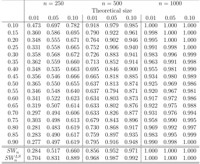
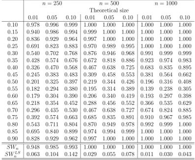
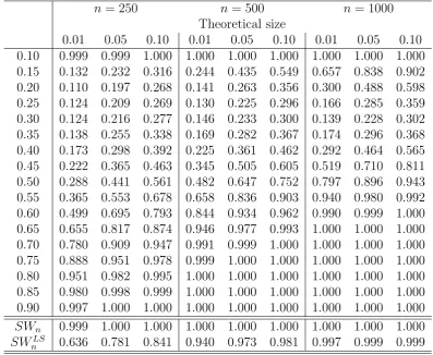
In order to evaluate the power of these tests we use two different sets of experiments. First, we assess the empirical power of the tests for three different two-regime models defined by different threshold nonlinearities (models 2, 3 and 4 below) in order to investigate advantages of quantile regression based tests versus least squares based tests. Second, we study the power of the test under local deviations from the linear null hypothesis. This family of models under the alternative hypothesis (model 5) is indexed by a local deviation parameter n−1/2c.
For the first power experiment, we consider the following three models:
Model 2:
Model 3:
yt=I(yt > γ0)(θ0+θ1yt−1+ (1 +δyt−1)ut) +I(yt≤γ0)(θ0+θ1yt−1 + (1−δyt−1)ut);
Model 4:
yt=I(yt > γ0)(θ0+θ1yt−1+ (1 +δyt−1)ut) +I(yt≤γ0)(θ0−θ1yt−1+ (1−δyt−1)ut).
Note that these data generating processes satisfy the following restrictions:
Model 2:
Qyt(τ|At−1) =
(θ0+ 2τ −1)−θ1yt−1, yt−1 ≤γ0,
(θ0+ 2τ −1) +θ1yt−1, yt−1 > γ0;
E[yt|At−1] =
θ0−θ1yt−1, yt−1 ≤γ0,
θ0+θ1yt−1, yt−1 > γ0;
Model 3:
Qyt(τ|At−1) =
(θ0+ 2τ −1) + (θ1−δ(2τ −1))yt−1, yt−1 ≤γ0,
(θ0+ 2τ −1) + (θ1+δ(2τ−1))yt−1, yt−1 > γ0;
E[yt|At−1] =
θ0+θ1yt−1, yt−1 ≤γ0,
θ0+θ1yt−1, yt−1 > γ0;
Model 4:
Qyt(τ|At−1) =
(θ0+ 2τ −1)−(θ1+δ(2τ −1))yt−1, yt−1 ≤γ0,
(θ0+ 2τ −1) + (θ1+δ(2τ−1))yt−1, yt−1 > γ0;
E[yt|At−1] =
θ0−θ1yt−1, yt−1 ≤γ0,
θ0+θ1yt−1, yt−1 > γ0.
Least squares based tests should be able to detect the presence of two regimes in models 2 and 4 where the threshold nonlinearity appears in the mean process, but not in model 3 where the mean process is identical in both regimes. Note that in models 3 and 4, the conditional variance process also exhibits a nonlinearity, that is, Var(yt|At−1, yt−1 ≤ γ0) 6= Var(yt|At−1, yt−1 > γ0). Quantile regression based tests,
In all these cases we use γ0 = 0, δ = 1, θ0 = 0, θ1 = 0.5 and ut ∼ i.i.d. U(−1,1).
In these models, xt= (1, yt−1)0, qt=yt−1 and At−1 ={yt−1, yt−2, . . .}.
The results for these three experiments are reported in Tables 2, 3 and 4, respec-tively. As expected, our proposed testSWnhas good power in all cases, and the power
is increasing in n, which is consistent with the theoretical result. SWnLS also shows power for models 2 and 4, but this test lacks statistical power to reject the null hy-pothesis if the nonlinearities are not in the mean process, that is, as in model 3. In all cases we observe that for the pointwise quantile tests the empirical power increases as we move to the tails of the distributions. These results suggest that the uniform test is very powerful to reject linearity for models exhibiting threshold nonlinearities in either the conditional mean or conditional variance processes.
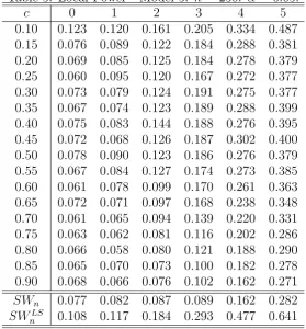
To complete the study of the power we perform a local power analysis: Model 5:
yt =I(yt> γ0)(θ0+(θ1+n−1/2c)yt−1+ut)+I(yt≤γ0)(θ0+(θ1−n−1/2c)yt−1+ut), (11)
where γ0 = 0, c∈ {0,1,2,3,4,5}, θ0 = 0, θ1 = 0.5, ut∼i.i.d. U(−1,1) and n= 250.
The simulation results appear in Table 5. Note that for this case, where the thresh-old nonlinearity appears in the mean process, the least squares based test is expected to be more powerful than the developed SWn test. In fact, the table shows that this
is the case. Nevertheless, the simulation results confirm that the proposed SWn test
performs well in local deviations from the null hypothesis. Unreported simulations show that the power function is symmetric with respect toc.
6
Summary
Acknowledgments
The authors would like to express their appreciation to Roger Koenker, Zhongjun Qu, Zhijie Xiao, and to the participants at the 2009 North American Summer Meeting of the Econometrics Society and the 2009 Far East and South Asia Meeting of the Econo-metrics Society for helpful comments and discussions. Kato’s research was partially supported by Grant-in-Aid for Young Scientists (B) (22730179) from the JSPS. Jose Olmo acknowledges financial support from Ministerio de Economia y Competitividad ECO2011-22650 project.
A
Proof of Theorem 1
In this section, we provide a proof of Theorem 1. The proof is based on a combination of modern empirical process techniques and the convexity technique developed in Kato (2009). Throughout the section, we assume all the conditions in Theorem 1.
A.1
Auxiliary result
For any fixed vector v∈Rd, define the stochastic processes
Un(τ, γ) :=
1
√
n
n
X
i=1
v0xtI(qt≤γ)[τ−I{yt≤x0tβ
∗
(1)(τ)}],
Vn(τ, γ, s) :=
1
√
n
n
X
i=1
v0xtI(qt≤γ)I{yt≤x0t(β
∗
(1)(τ) +sn
−1/2v)}
−E[v0xtI(qt ≤γ)F(x0t(β
∗
(1)(τ) +sn
−1/2v)|z
t)]
,
where (τ, γ, s)∈ T ×Γ×[0,1].
In this subsection, we study the asymptotic behaviors of Un and Vn. Let K(τ, λ)
denote a Kiefer process on [0,1] ×[0,∞), i.e., K(τ, λ) is a zero-mean, continuous Gaussian process on [0,1]×[0,∞) with covariance kernel
E[K(τ1, λ1)K(τ2, λ2)] =λ1 ∧λ2(τ1∧τ2−τ1τ2).
We refer to Section 2.12 of van der Vaart and Wellner (1996) for Kiefer processes. Define H(γ) := E[(v0xt)2I(qt ≤ γ)]. Under conditions (C2) and (C3), the map γ 7→
H(γ) is continuous and non-decreasing.
Theorem 3. Assume conditions (C1)-(C6). Then under H0,
(ii) Vn(τ, γ, s) = Vn(τ, γ,0) +op(1) uniformly over (τ, γ, s)∈ T ×Γ×[0,1].
Proof. Part (ii): We first prove Part (ii). For any compact subset B ⊂ Rd, consider
the class of functions
F :={f(y, q,x) =v0xI(q≤γ)I(y≤x0b) :γ ∈Γ,b∈B}.
We first show that F is a VC subgraph class. Indeed, let g(y, q,x) := v0x, F1 :=
{f(y, q,x) = I(q ≤ γ) : γ ∈ Γ} and F2 := {f(y, q,x) = I(y ≤ x0b) : b ∈ B}.
By Lemma 2.6.15 of van der Vaart and Wellner (1996), F1 and F2 are VC subgraph
classes. Therefore, by Lemmas 2.6.18 (i) and (vi) of van der Vaart and Wellner (1996),
F = (F1∧ F2)·g is a VC-subgraph class.
Define the semimetric
ρ((γ1,b1),(γ2,b2)) := E[|v0xt|p·|I(qt≤γ1)I(yt≤x0tb1)−I(qt≤γ2)I(yt≤x0tb2)|p]
1/p
,
wherep >2 is given in condition (C2). BecauseF is a VC subgraph class, by Theorem 2.1 of Arcones and Yu (1995) (more precisely their proof of Theorem 2.1), the stochastic process
(γ,b)∈Γ×B 7→√1
n
n
X
t=1
{v0xtI(qt≤γ)I(yt≤x0tb)−E[v
0
xtI(qt≤γ)F(x0tb|zt)]}
=:Gn(γ,b).
is stochastically ρ-equicontinuous over T ×Γ, i.e., for any >0,
lim
δ↓0 lim supn→∞
P
(
sup
[δ]
|Gn(γ1,b1)−Gn(γ2,b2)|>
)
= 0,
where [δ] :={((γ1,b1),(γ2,b2))∈(Γ×B)2 :ρ((γ1,b1),(γ2,b2))< δ}.
Observe now that
{ρ((γ1,b1),(γ2,b2))}p
≤E[|v0xt|p{I(qt≤γ1)I(yt≤x0tb1)−I(qt≤γ2)I(yt≤x0tb2)}2]
≤2E[|v0xt|p{I(qt ≤γ1)−I(qt ≤γ2)}2] + 2E[|v0xt|p· |F(x0tb1|zt)−F(x0tb2|zt)|]
By conditions (C3) and (C4), we have
sup
(τ,γ,s)∈T ×Γ×[0,1]
ρ((γ,β∗(1)(τ) +n−1/2sv),(γ,β(1)∗ (τ))) = o(1).
Recall that Vn(τ, γ, s) = Gn(γ,β(1)∗ (τ) +n−1/2sv). Thus, taking B sufficiently large
(so thatβ(1)∗ (τ) +n−1/2sv ∈B for all (τ, s)∈ T ×[0,1]), we obtain the first assertion
because of the stochasticρ-equicontinuity of the process Gn over Γ×B.
Part (i): Observe that under H0, {τ −I{yt ≤ x0tβ(1)∗ (τ)}, t ∈ Z} is a martingale
difference sequence with respect to {At−1, t∈ Z}, i.e., E[I{yt≤ x0tβ∗(1)(τ)}|At−1] =τ.
The finite dimensional convergence follows from the martingale central limit theorem. It remains to show the stochastic equicontinuity of the process Un. Decompose Un as
Un(τ, γ) =
τ √ n n X t=1
v0xtI(qt≤γ)−
1 √ n n X t=1
v0xtI(qt≤γ)I{yt ≤x0tβ
∗
(1)(τ)}
= √τ
n
n
X
t=1
{v0xtI(qt≤γ)−E[v0xtI(qt ≤γ)]} −Vn(τ, γ,0).
Define the stochastic process ˜Vn(γ) :=n−1/2
Pn t=1{v
0x
tI(qt≤γ)} −E[v0xtI(qt≤γ)]}.
Then Un(τ, γ) =τV˜n(γ)−Vn(τ, γ,0). By the previous calculation, we see that
ρ((γ1,β∗(1)(τ1)),(γ2,β∗(1)(τ2))) →0, as k(τ1−τ2, γ1−γ2)k →0,
which implies that the process (τ, γ)7→Vn(τ, γ,0) is stochastically equicontinuous over T ×Γ with respect to the Euclidean metric. Similarly, it is shown that the process
γ 7→V˜n(γ) is stochastically equiontinuous over Γ with respect to the Euclidean metric.
Therefore, by a standard argument, we obtain the desired conclusion.
A.2
Proof of Theorem 1
In this subsection, we provide a proof of Theorem 1. To this end, we introduce the local objective function
Zn(u, τ, γ) := n
X
t=1
ρτ yt−x0tβ
∗
(1)(τ)−n
−1/2u0z
t(γ)
−ρτ yt−x0tβ
∗
(1)(τ) ,
whereu∈R2dand (τ, γ)∈ T ×Γ. Observe that the normalized quantity√n{βˆ(τ, γ)− β∗(τ)} minimizes Zn(u, τ, γ) with respect to u for each fixed (τ, γ)∈ T ×Γ.
Kato (2009), it is sufficient to prove the following proposition.2
Proposition 2. Assume conditions (C1)-(C6). Then under H0,
Zn(u, τ, γ) = −
1 √ n n X t=1
τ −I{yt ≤x0tβ
∗
(1)(τ)}
u0zt(γ) +
1 2u
0
Ω1(τ, γ)u+ ∆n(u, τ, γ),
(12)
where sup(τ,γ)∈T ×Γ|∆n(u, τ, γ)|=op(1) for each fixed u∈R2d, and
1 √ n n X t=1
τ −I{yt≤x0tβ
∗
(1)(τ)}
zt(γ)⇒W(τ, γ) in (`∞(T ×Γ))2d. (13)
Proof. Using Knight’s (1998) identity
ρτ(x−y)−ρτ(x) =−y{τ −I(x≤0)}+y
Z 1
0
{I(x≤ys)−I(x≤0)}ds,
we decompose Zn(u, τ, γ) into three parts:
Zn(u, τ, γ)
=−√1
n
n
X
t=1
u0zt(γ)
τ −I{yt≤x0tβ
∗
(1)(τ)}
+ 1 n n X t=1
u0zt(γ)
Z 1
0
√
n[I{yt−x0tβ
∗
(1)(τ)≤n
−1/2
u0zt(γ)s)} −I{yt−x0tβ
∗
(1)(τ)≤0}]ds
=:Zn(1)(u, τ, γ) +Zn(2)(u, τ, γ)
=Zn(1)(u, τ, γ) + E[Zn(2)(u, τ, γ)] +{Zn(2)(u, τ, γ)−E[Zn(2)(u, τ, γ)]}
=:Zn(1)(u, τ, γ) +Zn(21)(u, τ, γ) +Zn(22)(u, τ, γ).
By Part (i) of Theorem 3, the weak convergence (13) follows. It remains to evaluate
Zn(21)(u, τ, γ) and Zn(22)(u, τ, γ).
Evaluation of Zn(21)(u, τ, γ): Observe that
Zn(21)(u, τ, γ) = E
u0zt(γ)
Z 1
0
√
n{F(x0tβ(1)∗ (τ) +sn−1/2u0zt(γ))|zt)−τ}ds
.
SinceF(x0tβ∗(1)(τ)|zt) = E[I{yt ≤x0tβ∗(1)(τ)}|zt] = E[E[I{yt≤x
0
tβ(1)∗ (τ)}|At−1]|zt] =τ
2In particular, Theorem 2 of Kato (2009) guarantees that there is no need to establish the uniform
under H0, we have
√
n{F(x0tβ(1)∗ (τ) +sn−1/2u0zt(γ))|zt)−τ} −su0zt(γ)f(x0tβ
∗
(1)(τ)|zt)
=su0zt(γ)
Z 1
0
{f(x0tβ(1)∗ (τ) +svn−1/2u0zt(γ)|zt)−f(x0tβ
∗
(1)(τ)|zt)}dv. (14)
Because of condition (C3), the right side of (14) goes to zero uniformly over (τ, γ, s)∈ T ×Γ×[0,1]. Therefore, by the dominated convergence theorem, we have
sup
(τ,γ)∈T ×Γ
Zn(21)(u, τ, γ)− 1
2u
0
Ω1(τ, γ)u
→0, ∀u∈R2d.
Evaluation of Zn(22)(u, τ, γ): Suppose for a moment thatu∈R2dis arbitrarily fixed.
Define
Rn(τ, γ, s) :=
1 √ n n X i=1
u0zt(γ)I{yt−x0tβ
∗
(1)(τ)≤sn
−1/2u0
zt(γ)}
−E[u0zt(γ)F(x0tβ
∗
(1)(τ) +sn
−1/2u0
zt(γ)|zt)]
,
where (τ, γ)∈ T ×Γ and s∈R. We shall show that
sup
(τ,γ)∈T ×Γ
sup
s∈[0,1]
|Rn(τ, γ, s)−Rn(τ, γ,0)| p
→0, (15)
which leads to sup(τ,γ)∈T ×Γ|Zn(22)(u, τ, γ)| p
→0. However, in view of
u0zt(γ) = (u1+u2)0xtI(qt≤γ) +u01xt{1−I(qt≤γ)},
(15) follows from Part (ii) of Theorem 3.
B
Conditions and proof for Proposition 1
B.1
Conditions for Proposition 1
We make the following conditions for Proposition 1.
(D1) For every n ≥ 1, the process {(yn,t,z0n,t)
0, t ∈
Z} is strict stationary and β
-mixing with β-mixing coefficients βn(j). Moreover, there exists a sequence of
non-increasing constants β(j) such that supn≥1βn(j)≤ β(j) and β(j) = O(j−l)
with l > p/(p−2), where p > 2 is given in condition (D2) below.
(D3) Let Fn(·|z) denote the conditional distribution function of yn,t given zn,t = z.
Assume that Fn(·|z) has a Lebesgue density fn(·|z) such that
(i) |fn(y|z)| ≤Cf, and
(ii) |fn(y1|z)−f(y2|z)| ≤Cf|y1−y2|,
where Cf >0 is a constant independent of n.
(D4) The distribution functions ofqn,t are continuous uniformly inn.
(D5) Define the matrices
Ωn,0(γ1, γ2) := E[zn,t(γ1)zn,t(γ2)0],
Ωn,2(τ, γ1, γ2) := E[fn(x0n,tβ
∗
(1)(τ)|zn,t)zn,t(γ)zn,t(γ)0], Ωn,1(τ, γ) := Ωn,2(τ, γ, γ).
There exist d×d matrices Ω0(γ1, γ2) and Ω2(τ, γ1, γ2) such that Ωn,0(γ1, γ2) →
Ω0(γ1, γ2) and Ωn,2(τ, γ1, γ2) → Ω2(τ, γ1, γ2) uniformly over (γ1, γ2) ∈ Γ × Γ
and (τ, γ1, γ2) ∈ T ×Γ×Γ, respectively. Moreover, Ω0(γ1, γ2) and Ω1(τ, γ) :=
Ω2(τ, γ, γ) are positive definite uniformly over (γ1, γ2)∈Γ×Γ and (τ, γ)∈ T ×Γ,
respectively.
B.2
Proof of Proposition 1
As in the proof of Theorem 1, define
Zn(u, τ, γ) := n
X
t=1
ρτ yn,t−x0n,tβ
∗
(1)(τ)−n
−1/2u0
zn,t(γ)
−ρτ yn,t−x0n,tβ
∗
(1)(τ) ,
where u∈R2d and (τ, γ)∈ T ×Γ. An inspection of the proof of Proposition 2 shows
that under H1n, we still have the expansion
Zn(u, τ, γ) =−
1 √ n n X t=1
τ−I{yn,t≤x0n,tβ
∗
(1)(τ)}
u0zn,t(γ)+
1 2u
0
Ω1(τ, γ)u+∆n(u, τ, γ),
where sup(τ,γ)∈T ×Γ|∆n(u, τ, γ)| = op(1) for each fixed u ∈ R2d. Here the difference
arises since τ −I{yn,t ≤x0n,tβ
∗
(1)(τ)} are not centered. Fixu ∈R
2d, and define
Zn(1)(τ, γ) = √1
n
n
X
t=1
τ −I{yn,t ≤x0n,tβ
∗
(1)(τ)}
Let us write β∗n(τ) = (β∗(1)(τ)0,β(2),n(τ)0)0 where β(2),n(τ) =n−1/2c(τ). Observe that
Zn(1)(τ, γ) = √1
n
n
X
t=1
[τ−I{yn,t≤zn,t(γ0)0β∗n(τ)}]u
0
zn,t(γ)
+√1
n
n
X
t=1
I{yn,t ≤zn,t(γ0)0βn∗(τ)} −I{yn,t≤x0n,tβ
∗
(1)(τ)}
u0zn,t(γ)
=:Zn(11)(τ, γ) +Zn(12)(τ, γ)
=Zn(11)(τ, γ) + E[Zn(12)(τ, γ)] +Zn(12)(τ, γ)−E[Zn(12)(τ, γ)]
=:Zn(11)(τ, γ) + E[Zn(12)(τ, γ)] +Zn(13)(τ, γ).
By Theorem 3 (with suitable modifications), we can show that
1
√
n
n
X
t=1
τ −I{yn,t ≤zn,t(γ0)0β(∗n)(τ)}
zn,t(γ)⇒W(τ, γ), in (`∞(T ×Γ))2d,
where W(τ, γ) is as in Theorem 1 (with Ω0(γ1, γ2) replaced by (7)), and
sup
(τ,γ)∈T ×Γ
|Zn(13)(τ, γ)|=op(1).
By using Taylor’s theorem, we also have
E[Zn(12)(τ, γ)] = u0E[fn(x0n,tβ(1)(τ)|zn,t)zn,t(γ)zn,t(γ0)0]R0c(τ) +o(1)
=u0Ω2(τ, γ, γ0)R0c(τ) +o(1).
uniformly over (τ, γ)∈ T ×Γ. Hence by Theorem 2 of Kato (2009), we conclude that
√
n{βˆ(τ, γ)−(β∗(1)(τ)0,00)0} ⇒Ω1(τ, γ)−1(W(τ, γ)+Ω2(τ, γ, γ0)R0c(τ)), in (`∞(T ×Γ))2d,
which implies the conclusion of the proposition.
C
Proofs for Section 4
C.1
Proof of Lemma 2
We only provide a sketch of the proof. It is standard to show that when the ob-servations are independent and identically distributed, ˆΩ0(γ1, γ2) → Ω0(γ1, γ2)
al-most surely uniformly over (γ1, γ2) ∈ Γ ×Γ. By Theorem 1 of Nobel and Dembo
(1993), the uniform consistency of ˆΩ0(γ1, γ2) now follows under the present
theo-rem of Nobel and Dembo (1993), it is shown that ˜β1(τ) is uniformly consistent:
supτ∈T kβ˜(1)(τ)−β(1)∗ (τ)k
p
→0. The proof of the uniform consistency of ˆΩ1(τ, γ) is
sim-ilar to the proof given in Appendix A.1.4 of Angrist et al. (2006). Fix any 1≤j, k ≤d. For any compact subset B ⊂ Rd and positive constant H, consider the class of
func-tions F := {f(y, q,x) = I(|y−x0b| ≤ h)I(q ≤ γ)xjxk : γ ∈ Γ,b ∈ B, h ∈ (0, H]},
where x= (x1, . . . , xd)0. As in the proof of Theorem 3, it is shown that the class F is
a VC subgraph class. Using the uniform central limit theorem forβ-mixing processes (Arcones and Yu, 1995, Theorem 2.1), and following the proof given in Appendix A.1.4 of Angrist et al. (2006), it is shown that, under the present conditions,
1 2nhn
n
X
t=1
I(|yt−x0tβ˜(1)(τ)| ≤hn)I(qt≤γ)xtjxtk
= 1 2hn
E [I(|yt−x0tb| ≤hn)I(qt≤γ)xtjxtk]|b= ˜β(1)(τ)+Op(n
−1/2h−1
n )
= E[f(x0tβ(1)∗ (τ)|zt)I(qt ≤γ)xtjxtk] +op(1),
and the convergence is uniform over (τ, γ)∈ T ×Γ. With the same proof, it is shown that, uniformly overτ ∈ T,
1 2nhn
n
X
t=1
I(|yt−x0tβ˜(1)(τ)| ≤hn)xtjxtk p
→E[f(x0tβ∗(1)(τ)|zt)xtjxtk].
Therefore, we have ˆΩ1(τ, γ)
p
→Ω1(τ, γ) uniformly over (τ, γ)∈ T ×Γ.
C.2
Proof of Theorem 2
n)→1, so that
P(SWn>ˆc∗1−α)
= P({SWn >cˆ∗1−α} ∩ {ˆc
∗
1−α ≥c1−α−n}) +o(1) ≤P(SWn> c1−α−n) +o(1)
≤P(SW > c1−α−n) + [P(SWn > c1−α−n)−P(SW > c1−α−n)] +o(1) ≤P(SW > c1−α−n) + sup
c∈R
|P(SWn> c)−P(SW > c)|+o(1)
= P(SW > c1−α−n) +o(1),
where the last equality follows from the fact that SWn ⇒ SW under H0, SW has
a continuous distribution and Polya’s theorem. Because SW has a bounded density function, we have P(SW > c1−α−n) = P(SW > c1−α) +o(1) = α+o(1), so that
P(SWn > ˆc∗1−α) ≤ α +o(1). A similar argument leads to that P(SWn > ˆc∗1−α) ≥
α−o(1), which implies (i). By an analogous argument, it is shown that (iii) follows from (i).
In what follows, we wish to show (i). To this end, we need the concept of “con-ditional weak convergence in probability”. We follow the definition given in van der Vaart and Wellner (1996, p.181). We wish to show that, given {(yt,zt0)
0}n
i=1, SWd
∗
n
converges weakly to SW in probability. Once this is established, the assertion of (i) follows because of the fact that the quantile function ofSW is everywhere continuous by Theorem 11.1 (iv) of Davidov et al. (1998) (recall that the distribution function of
SW is continuous). By a standard argument, it suffices to show that, given{zt}nt=1, in
the space (`∞(T ×Γ))2d, Wn∗ converges weakly in probability to the Gaussian process
W defined in Theorem 1.
We adapt the proof of van der Vaart and Wellner (1996, Theorem 2.9.6) to the present context (some modifications are required because the situation is different from that theorem; in particular, z1, . . . ,zn are now dependent and the quantile index
τ is involved in the simulated termI(u∗t ≤τ), so their Lemma 2.9.1 can not be used in the present case). Introduce any normk·k(`∞(T ×Γ))2d on (`∞(T ×Γ))2dthat induces the
topology of (`∞(T ×Γ))2d (for example, take kfk
(`∞(T ×Γ))2d = sup(τ,γ)∈T ×Γkf(τ, γ)k
forf ∈(`∞(T ×Γ))2d). LetBL
1 denote the space of all Lipschitz continuous functions
(`∞(T ×Γ))2d→[−1,1] with Lipschitz constant bounded by 1. We have to show that
sup
h∈BL1
|E[h(Wn∗)|z1n]−E[h(W)]|→p 0,
where zn
Step 1: Because T ×Γ is compact in R2, for any δ > 0, there exists a finite set
{(τk, γk)}kK=1 such that sup(τ,γ)∈T ×Γmin1≤k≤Kk(τ, γ)−(τk, γk)k ≤δ. Let Πδdenote the
map fromT ×Γ to{(τk, γk)}Kk=1 such thatk(τ, γ)−Πδ(τ, γ)k ≤δ for all (τ, γ)∈ T ×Γ.
Define the stochastic processW ◦Πδ onT ×Γ by W ◦Πδ(τ, γ) :=W(Πδ(τ, γ)). Then
becauseW is uniformly continuous onT ×Γ, asδ ↓0,W◦Πδ→W in (`∞(T ×Γ))2d.
Therefore, by the dominated convergence theorem, we have
lim
δ↓0 hsup∈BL1|E[h(W ◦Πδ)]−E[h(W)]|= 0. (16)
Step 2: Fix anyδ >0. We wish to show that, withWn∗◦Πδ(τ, γ) := Wn∗(Πδ(τ, γ)),
sup
h∈BL1
|E[h(Wn∗◦Πδ)|z1n]−E[h(W ◦Πδ)]| p
→0. (17)
To this end, it suffices to show that conditionally on z1,z2, . . .,
(Wn∗(τk, γk))1≤k≤K d
→(W(τk, γk))1≤k≤K, (18)
for almost every sequencez1,z2, . . .. Because of the ergodicity, we have: (a) ˆΩ0(γk, γl) =
n−1Pn
t=1zt(γk)zt(γl)0 → Ω0(γk, γl) for all 1 ≤ k, l ≤ K almost surely, and (b)
max1≤t≤nkxtk/ √
n→0 almost surely. On the intersection of these two events (events (a) and (b)), it is shown by the Lindberg-Feller central limit theorem that (18) holds conditionally on z1,z2, . . .. Therefore, we obtain the desired claim.
Step 3: We wish to show that
lim
δ↓0 nlim→∞E
sup
h∈BL1
|E[h(Wn∗)|zn1]−E[h(Wn∗ ◦Πδ)|z1n]|
= 0. (19)
Observe that|E[h(Wn∗)|z1n]−E[h(Wn∗◦Πδ)|z1n]| ≤E[|h(W
∗
n)−h(W
∗
n◦Πδ)||z1n], so that
E
sup
h∈BL1
|E[h(Wn∗)|zn1]−E[h(Wn∗◦Πδ)|z1n]|
≤E
sup
h∈BL1
|h(Wn∗)−h(Wn∗◦Πδ)|
.
By essentially the same proof as that of Theorem 3, it is shown that Wn∗ ⇒ W in (`∞(T ×Γ))2d unconditionally. Thus, by Theorem 1.5.7 of van der Vaart and Wellner
(1996), for any >0, there exist a constant δ=δ >0 and a positive integer n such
that for all n ≥n,
PkWn∗−Wn∗◦Πδk(`∞(T ×Γ))2d > ≤.
the event A0, |h(Wn∗)−h(W
∗
n ◦Πδ)| ≤ kWn∗ −W
∗
n ◦Πδk(`∞(T ×Γ))2d ≤ , while on the
event Ac
0,|h(W
∗
n)−h(W
∗
n◦Πδ)| ≤2. Observe that P(Ac0)≤. Therefore, we have
E
sup
h∈BL1
|h(Wn∗)−h(Wn∗◦Πδ)|
≤3.
This implies (19).
Finally, for any δ > 0,
sup
h∈BL1
|E[h(Wn∗)|zn1]−E[h(W)]| ≤ sup
h∈BL1
|E[h(Wn∗)|zn1]−E[h(Wn∗◦Πδ)|z1n]|
+ sup
h∈BL1
|E[h(Wn∗◦Πδ)|zn1]−E[h(W ◦Πδ)]|
+ sup
h∈BL1
|E[h(W ◦Πδ)]−E[h(W)]|.
The expectation of the first term on the right side goes to zero as letting n→ ∞ first and then δ ↓0 by (19); the expectation of the second term goes to zero asn → ∞ by (17) and the dominated convergence theorem; and the last term goes to zero as δ ↓ 0 by (16). Therefore, we have
E
sup
h∈BL1
|E[h(Wn∗)|z1n]−E[h(W)]|
→0.
By Markov’s inequality, we obtain the desired conclusion.
References
Andrews, D.W.K. (1991). Heteroskedasticity and autocorrelation consistent covariance matrix estimation.Econometrica 59 817-858.
Andrews, D.W.K. and Ploberger, W. (1994). Optimal tests when a nuisance parameter is present only under the alternative.Econometrica 62 1383-1414.
Angrist, J., Chernozhukov, V. and Fern´andez-Val, I. (2006). Quantile regression under misspecification, with an application to the US wage structure. Econometrica 74
539-563.
Cai, Y. (2010). Forecasting for quantile self-exciting threshold autoregressive time series models.Biometrika 97 199-208.
Cai, Y. and Stander, J. (2008). Quantile self-exciting threshold time series models. J. Time Series Anal.29 187-202.
Caner, M. (2002). A note on least absolute deviation estimation of a threshold model.
Econometric Theory 18 800-814.
Carrasco, M. (2002). Misspecified structural change, threshold, and Markov-switching models.J. Econometrics 109 239-273.
Chan, K.S. (1990). Testing for threshold autoregression.Ann. Statist. 18 1886-1894.
Chernozhukov, V. and Fern´andez-Val, I. (2005). Subsampling inference on quantile regression processes.Sankhya 67 253-276.
Davidov, Y., Lifshits, M. and Smorodina, N. (1998). Local Properties of Distributions of Stochastic Functions(Transaction of Mathematical Monographs, Vol. 173). Amer-ican Mathematical Society.
Davies, R. (1977). Hypothesis testing when a nuisance parameter is present only under the alternative.Biometrika 64 247-254.
Davies, R. (1987). Hypothesis testing when a nuisance parameter is present only under the alternative.Biometrika 74 33-43.
Escanciano, J.C. and Velasco, C. (2010). Specification tests of parametric dynamic conditional quantiles.J. Econometrics 159 209-221.
Fan, J. and Yao, Q. (2005). Nonlinear Time Series: Nonparametric and Parametric Methods. Springer-Verlag.
Gutenbrunner, C. and Jureˇckov´a, J. (1992). Regression rank scores and regression quantiles. Ann. Statist. 20 305-330.
Hansen, B.E. (1996). Inference when a nuisance parameter is not identified under the null hypothesis. Econometrica 64 413-430.
Hansen, B.E. (1997). Inference in TAR models.Stud. Nonlinear Dyn. Econom.21-14.
He, X. and Zhu, L.X. (2003). A lack-of-fit test for quantile regression. J. Amer. Stat. Assoc.98 1013-1022.
Horowitz, J.L. and Spokoiny, V.G. (2002). An adaptive, rate-optimal test of linearity of median regression models.J. Amer. Stat. Assoc. 97 822-835.
Kato, K. (2009). Asyptotics for argmin processes: convexity arguments.J. Multivariate Anal. 100 1816-1829.
Knight, K. (1998). Limiting distribution for L1 regression estimators under general
conditions.Ann. Statist. 26 755-770.
Koenker, R. (2005). Quantile Regression. Cambridge University Press.
Koenker, R. and Bassett, G. (1978). Regression quantiles. Econometrica 46 33-50.
Koenker, R. and Machado, J.A.F. (1999). Goodness-of-fit and related inference pro-cesses for quantile regression. J. Amer. Stat. Assoc. 94 1296-1310.
Koenker, R. and Xiao, Z. (2002). Inference on the quantile regression process. Econo-metrica 70 1583-1612.
Komunjer, I. and Vuong, Q. (2010a). Semiparametric efficiency bound in time-series models for conditional quantiles.Econometric Theory 26 383-405.
Komunjer, I. and Vuong, Q. (2010b). Efficient estimation in dynamic conditional quan-tile models. J. Econometrics 157 272-285.
Lee, S., Seo, M.H. and Shin, Y. (2011). Testing for threshold effects in regression models.J. Amer. Stat. Assoc. 106 220-231.
Nobel, A. and Dembo, A. (1993). A note on uniform laws of averages for dependent processes.Statist. Probab. Lett. 17 169-172.
Otsu, T. (2008). Conditional empirical likelihood estimation and inference for quantile regression. J. Econometrics 142 508-538.
Powell, J.L. (1991). Estimation of monotonic regression models under quantile re-strictions. In: Nonparametric and Semiparametric Models in Econometrics(eds. W. Barnett, J.L. Powell and G. Tauchen). Cambridge University Press.
Su, L. and Xiao, Z. (2008). Testing for parameter stability in quantile regression models.
Statist. Probab. Lett.78 2768-2775.
Su, L. and White, H. (2012). Conditional independence specification testing for depen-dent processes with local polynomial quantile regression.Advances in Econometrics 29 355-434.
Tong, H. (1983).Threshold Models in Non-linear Time Series Analysis(Lecture Notes in Statistics). Springer-Verlag.
Tong, H. and Lim, K. (1980). Threshold autoregression, limit cycles and cyclical data.
J. Roy. Stat. Soc. Ser. B Stat. Methodol.4 245-292.
Tsay, R. (1989). Testing and modeling threshold autoregressive processes. J. Amer. Stat. Assoc.18 931-955.
van der Vaart, A.W. and Wellner, J.A. (1996).Weak Convergence and Empirical Pro-cesses: With Applications to Statistics. Springer-Verlag.
Whang, Y.-J. (2005). Consistent specification testing for quantile regression models. In:
Frontiers of Analysis and Applied Research: Essays in Honor of Peter C.B. Phillips
(eds. D. Corbae, S.N. Durlauf, and B.E. Hansen). Cambridge University Press.
Tables
Table 1: Size - One-regime AR(1) model
n= 250 n = 500 n = 1000 Theoretical size
0.01 0.05 0.10 0.01 0.05 0.10 0.01 0.05 0.10 0.10 0.058 0.135 0.204 0.034 0.109 0.154 0.037 0.099 0.173 0.15 0.033 0.074 0.106 0.011 0.027 0.042 0.006 0.021 0.036 0.20 0.021 0.059 0.091 0.012 0.037 0.066 0.007 0.036 0.065 0.25 0.026 0.057 0.096 0.009 0.049 0.095 0.019 0.055 0.106 0.30 0.024 0.072 0.119 0.016 0.060 0.111 0.025 0.077 0.157 0.35 0.025 0.086 0.139 0.026 0.069 0.137 0.033 0.090 0.160 0.40 0.019 0.078 0.147 0.036 0.094 0.160 0.029 0.094 0.172 0.45 0.027 0.092 0.158 0.033 0.104 0.173 0.032 0.088 0.154 0.50 0.031 0.112 0.174 0.045 0.111 0.182 0.032 0.097 0.169 0.55 0.030 0.094 0.173 0.046 0.105 0.172 0.030 0.093 0.157 0.60 0.025 0.102 0.150 0.044 0.098 0.177 0.037 0.097 0.153 0.65 0.020 0.079 0.144 0.036 0.107 0.177 0.034 0.109 0.163 0.70 0.020 0.078 0.135 0.021 0.094 0.160 0.041 0.097 0.152 0.75 0.023 0.067 0.118 0.022 0.060 0.139 0.022 0.077 0.130 0.80 0.022 0.069 0.135 0.016 0.062 0.113 0.018 0.068 0.129 0.85 0.037 0.078 0.119 0.016 0.049 0.088 0.019 0.056 0.107 0.90 0.038 0.080 0.118 0.015 0.035 0.073 0.014 0.042 0.079
SWn 0.040 0.076 0.109 0.011 0.033 0.060 0.015 0.032 0.053
SWLS
Table 2: Power - Model 2
n= 250 n = 500 n = 1000 Theoretical size
0.01 0.05 0.10 0.01 0.05 0.10 0.01 0.05 0.10 0.10 0.473 0.697 0.782 0.918 0.979 0.985 1.000 1.000 1.000 0.15 0.360 0.586 0.695 0.790 0.922 0.961 0.998 1.000 1.000 0.20 0.348 0.555 0.671 0.764 0.902 0.946 0.995 1.000 1.000 0.25 0.331 0.558 0.665 0.752 0.906 0.940 0.991 0.998 1.000 0.30 0.358 0.568 0.672 0.726 0.883 0.941 0.983 0.996 0.999 0.35 0.362 0.559 0.660 0.713 0.852 0.914 0.963 0.991 0.998 0.40 0.348 0.535 0.663 0.695 0.846 0.900 0.955 0.981 0.990 0.45 0.356 0.546 0.666 0.665 0.818 0.885 0.934 0.980 0.989 0.50 0.365 0.550 0.655 0.637 0.813 0.874 0.925 0.969 0.986 0.55 0.346 0.548 0.640 0.637 0.794 0.871 0.920 0.967 0.981 0.60 0.341 0.522 0.623 0.634 0.803 0.873 0.917 0.972 0.986 0.65 0.319 0.507 0.614 0.633 0.802 0.876 0.922 0.975 0.988 0.70 0.297 0.494 0.606 0.633 0.826 0.877 0.931 0.976 0.994 0.75 0.303 0.498 0.613 0.679 0.843 0.896 0.958 0.990 0.995 0.80 0.281 0.483 0.619 0.730 0.868 0.917 0.969 0.992 0.997 0.85 0.283 0.490 0.617 0.759 0.897 0.935 0.983 0.995 0.999 0.90 0.277 0.497 0.619 0.795 0.916 0.948 0.990 0.998 1.000
SWn 0.284 0.517 0.660 0.856 0.952 0.971 1.000 1.000 1.000
SWLS
Table 3: Power - Model 3
n= 250 n = 500 n = 1000 Theoretical size
0.01 0.05 0.10 0.01 0.05 0.10 0.01 0.05 0.10 0.10 0.978 0.996 0.999 1.000 1.000 1.000 1.000 1.000 1.000 0.15 0.940 0.986 0.994 0.999 1.000 1.000 1.000 1.000 1.000 0.20 0.836 0.929 0.964 0.997 1.000 1.000 1.000 1.000 1.000 0.25 0.691 0.823 0.883 0.970 0.989 0.995 1.000 1.000 1.000 0.30 0.540 0.702 0.768 0.876 0.946 0.968 0.991 0.999 0.999 0.35 0.428 0.574 0.676 0.672 0.818 0.886 0.923 0.974 0.983 0.40 0.326 0.470 0.568 0.467 0.638 0.725 0.683 0.835 0.895 0.45 0.245 0.383 0.483 0.309 0.458 0.553 0.381 0.564 0.662 0.50 0.201 0.325 0.397 0.219 0.344 0.426 0.196 0.316 0.408 0.55 0.182 0.294 0.380 0.195 0.314 0.389 0.139 0.238 0.305 0.60 0.179 0.304 0.390 0.206 0.340 0.419 0.193 0.297 0.398 0.65 0.218 0.354 0.452 0.288 0.456 0.552 0.366 0.535 0.629 0.70 0.296 0.435 0.530 0.467 0.638 0.727 0.674 0.824 0.885 0.75 0.392 0.574 0.663 0.685 0.835 0.891 0.910 0.967 0.985 0.80 0.543 0.711 0.804 0.870 0.949 0.978 0.992 0.999 1.000 0.85 0.695 0.840 0.899 0.974 0.994 0.999 1.000 1.000 1.000 0.90 0.828 0.929 0.962 0.997 1.000 1.000 1.000 1.000 1.000
SWn 0.948 0.985 0.993 1.000 1.000 1.000 1.000 1.000 1.000
SWLS
Table 4: Power - Model 4
n= 250 n = 500 n = 1000 Theoretical size
0.01 0.05 0.10 0.01 0.05 0.10 0.01 0.05 0.10 0.10 0.999 0.999 1.000 1.000 1.000 1.000 1.000 1.000 1.000 0.15 0.132 0.232 0.316 0.244 0.435 0.549 0.657 0.838 0.902 0.20 0.110 0.197 0.268 0.141 0.263 0.356 0.300 0.488 0.598 0.25 0.124 0.209 0.269 0.130 0.225 0.296 0.166 0.285 0.359 0.30 0.124 0.216 0.277 0.146 0.233 0.300 0.139 0.228 0.302 0.35 0.138 0.255 0.338 0.169 0.282 0.367 0.174 0.296 0.368 0.40 0.173 0.298 0.392 0.225 0.361 0.462 0.292 0.464 0.565 0.45 0.222 0.365 0.463 0.345 0.505 0.605 0.519 0.710 0.811 0.50 0.288 0.441 0.561 0.482 0.647 0.752 0.797 0.896 0.943 0.55 0.365 0.553 0.678 0.658 0.836 0.903 0.940 0.980 0.992 0.60 0.499 0.695 0.793 0.844 0.934 0.962 0.990 0.999 1.000 0.65 0.655 0.817 0.874 0.946 0.977 0.993 1.000 1.000 1.000 0.70 0.780 0.909 0.947 0.991 0.999 1.000 1.000 1.000 1.000 0.75 0.888 0.951 0.978 0.999 1.000 1.000 1.000 1.000 1.000 0.80 0.951 0.982 0.995 1.000 1.000 1.000 1.000 1.000 1.000 0.85 0.980 0.998 0.999 1.000 1.000 1.000 1.000 1.000 1.000 0.90 0.997 1.000 1.000 1.000 1.000 1.000 1.000 1.000 1.000
SWn 0.999 1.000 1.000 1.000 1.000 1.000 1.000 1.000 1.000
SWLS
Table 5: Local Power - Model 5. n= 250. α= 0.05.
c 0 1 2 3 4 5
0.10 0.123 0.120 0.161 0.205 0.334 0.487 0.15 0.076 0.089 0.122 0.184 0.288 0.381 0.20 0.069 0.085 0.125 0.184 0.278 0.379 0.25 0.060 0.095 0.120 0.167 0.272 0.377 0.30 0.073 0.079 0.124 0.191 0.275 0.377 0.35 0.067 0.074 0.123 0.189 0.288 0.399 0.40 0.075 0.083 0.144 0.188 0.276 0.395 0.45 0.072 0.068 0.126 0.187 0.302 0.400 0.50 0.078 0.090 0.123 0.186 0.276 0.379 0.55 0.067 0.084 0.127 0.174 0.273 0.385 0.60 0.061 0.078 0.099 0.170 0.261 0.363 0.65 0.072 0.071 0.097 0.168 0.238 0.348 0.70 0.061 0.065 0.094 0.139 0.220 0.331 0.75 0.063 0.062 0.081 0.116 0.202 0.286 0.80 0.066 0.058 0.080 0.121 0.188 0.290 0.85 0.065 0.070 0.073 0.100 0.182 0.278 0.90 0.068 0.066 0.076 0.102 0.162 0.271
SWn 0.077 0.082 0.087 0.089 0.162 0.282
SWLS