A symplectic analytical singular element for steady-state thermal conduction with singularities in composite structures

A symplectic analytical singular element for steady-state thermal conduction with singularities in composite structures

XF Hua, HY Gaob, WA Yaoa*, ST Yangc

a _{State Key Laboratory of Structural Analysis for Industrial Equipment, Dalian University of Technology, Dalian}

116024, China

b _{Beijing Institute of Spacecraft Environment Engineering, Beijing, China}

c _{Department of Civil and Environmental Engineering, the University of Strathclyde, Glasgow, G1 1XJ, United}

Kingdom

*_{Corresponding author: [email protected]}

Abstract: In modern design of composite structures, multiple materials with different properties are bounded together. Accurate prediction of the strength of the interface between different materials, especially with the existence of cracks under thermal loading, is demanded in engineering. To this end, detailed knowledge on the distribution of temperature and heat flux is required. This study conducts a systematical investigation on the cracks terminated at material interface under steady-state thermal conduction. A new symplectic analytical singular element is constructed for the numerical modeling. Combining the proposed element with conventional finite elements the generalized flux intensity factors can be solved accurately.

Nomenclature

,

A B coefficients of the general solution of symplectic eigenvector

F vector of coefficients of the general solution of symplectic eigenvector

H Hamiltonian operator matrix

k thermal conductivity

i

M (i=1, 2,3) material

r

q , q_θ heat flux densities

R chain matrix relates the eigenvectors of two adjacent materials

r

S , S_θ symplectic dual variables

T temperature

Z unknown vector in symplectic solving system

α

vertex angle of material

( , )r

θ

polar coordinate system

2

∇ Laplacian operator

µ symplectic eigenvalue

( )θ

ψ symplectic eigenvector

,

T r

ψ ψ elements in symplectic eigenvector

γ _{coefficients of symplectic eigen expanding terms}

Θ expression of characteristic equation of symplectic eigenvalue

1. Introduction

Composite materials fabricated by combining two or more different materials are widely applied in engineering for their advantages which are not attainable by any single engineering material. However, extensive amount of interfaces between two different materials exist in such composite materials which will possibly lead to delamination under thermal loading. For some cases, delamination migrates to the adjacent interface in terms of a inclined crack terminated at the material interface[1]. According to the previous study, it is known that not only stresses but also heat flux density possess singularity in the vicinity of a crack tip[2].

Many contributions have been reported in existing literatures. Kou studied bimaterial interface crack between two semi-infinite dissimilar media subject to uniform heat flow, and obtained the temperature distribution[3]. Chao and Chang investigated interface crack between dissimilar anisotropic media based on the Hilbert problem formulation and a special technique of analytical continuation, and obtained the analytical solution for steady-state heat conduction problem[4]. Chao et al. studied heat conduction of curvilinear cracks in bounded dissimilar materials with heat source[5]. Marin proposed an invariant method of fundamental solutions to investigated 2D steady-state anisotropic heat conduction problems[6]. Hasebe and Kato reported a closed-form solution for the bonded bimaterial planes at two interfaces subject to different temperatures[7].

For more general problems numerical methods such as finite element method (FEM) and boundary element method (BEM) should be employed to get numerical predictions. Ling and Yang proposed a virtual boundary meshless with Trefftz method to investigate the two dimensional (2D) steady-state heat conduction problem for cracks and the heat stress intensity factor can be simply calculated[8]_{. Zhou et al.,}

proposed a new numerical method for study of steady-state thermal conduction problem of bimaterial interface cracks[9]. Yosibash and his collaborators investigated systematically on the steady-state thermal conduction problems with singularities, numerical solutions of the generalized flux intensity factors(GFIF) were obtained based on post process operations in conjunction with FEM[10, 11, 12, 13]. Yvonnet et al. investigated the Kapitza thermal resistance between two three dimensional (3D) dissimilar materials by using extended finite element method (XFEM) in which the temperature jump across the interface can be captured accurately with the aid of analytical solution[14].

material[17, 18], and multi-material cracks under mechanical loading[19] were obtained. Based on the symplectic eigen solutions, a series of analytical singular elements were constructed for the numerical study of cracks[20]_{, fatigue crack growth}[21]_{, cracks in Reissner plate}[22] _{and Dugdale cohesive model}

based cracks[23]. Leung et al. employed the symplectic dual approach to the study of steady-state thermal conduction problem analytically and numerically[24, 25]. And for the case of inclined crack terminated at the material interface, the states of stresses and temperatures are even more complex. As a result, it brings significant challenge on both analytical study and numerical modeling of the progressive damage in composite materials under thermal loading.

In the light of existing numerical methods for steady-state thermal conduction with singularities, the combination of near crack tip asymptotic solution and conventional numerical methods such as FEM brings many advantages. The rich information of thermal variables expressed in terms of eigen solution should be applied to benefit the solving accuracy and efficiency. Motivated by this, the present study first attempts to find the analytical symplectic eigen solution of steady-state thermal conduction in inclined crack terminated at bimaterial interface. A symplectic analytical singular element (SASE) is also developed for numerical simulation.

2. Fundamental equations

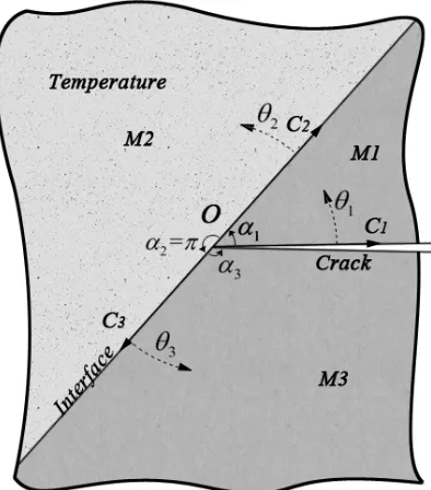
Considering an inclined bimaterial crack terminated at the material interface as shown in Fig.1,

each material is represented by Mi(i=1, 2,3) where M M1= 3 represents the same material while M2

represents the other material. The subscript "₃" is introduced to distinguish the different parts of material

1 separated by the crack. So the vertex angles satisfy α α1+ 3=π, and α2=π. Each part of the material can

be described under the sub polar coordinate system

OC

_{i i}

θ

as shown in Fig.1.

In terms of steady-state thermal conduction problem, the relationship between temperature and heat

flux densities in material Mi can be specified by:

, i

r i i

T q k r ∂ =− ∂ , , i i i i k T q r θ θ ∂ =−

∂ (i=1, 2,3) (1)

where T_i is temperature and [q qr i,, θ,i] is the vector of heat flux densities along each direction, and ki is

thermal conductivity. The steady-state heat conduction equation in the absence of the internal heat source can be expressed in terms of temperature using the Laplacian operator 2

∇ as:

2 ₀

i T

whereas the Laplacian operator in the polar coordinate system is 2 2 _{(1/ ) (1/ )}2 2

r r r r θ

∇ =∂ + ∂ + ∂ . The

interface between the two materials is assumed to be perfect bounded and the compatibility conditions at the interface are specified by

1

1 0

|_{i i} |_i

i i

T _{θ α} T _θ

+

= = + = ( 1, 2)i= (3)

1 ,i|_{i i} , 1i |_i 0

q_{θ θ α} q_{θ θ}

+

= = + = ( 1, 2)i= (4)

The fundamental equations can also be derived from the following equation of dissipation of quantity of heat specified by:

0 0

3

, 2 2

, , ,

1

δ 1 ( ) d d 0

2

i i i i

r i r i i i

i i i

q

T T

q q q r r

r r k

α _θ θ θ θ ∞ = ⎧ ⎛ ∂ ∂ ⎞ ⎫ ⎪ ⎪ + + + = ⎨ ⎜ _{∂ ∂} ⎟ ⎬ ⎪ ⎝ ⎠ ⎪ ⎩

∑

∫ ∫

⎭ (5)

Typical boundary conditions at the crack surfaces are combinations of specific temperature and/or heat flux density, and the standard homogeneous boundary conditions can be summarized as

(i) prescribed temperature: T1|θ₁=0=0, |T3 θ α₃= ₃=0 (6)

(ii) prescribed temperature and heat flux:

1 3 3

1 0 0, 3/ 3 0

T T

θ= = ∂ ∂

θ

θ α= = (7)

(iii) prescribed heat flux:

1 3 3

1/ 1 0 0, 3/ 3 0

T T

θ θ α

θ

₌

θ

₌

∂ ∂ = ∂ ∂ = (8)

The subscripts "₁", "₂" and "₃" will be omitted hereinafter except where it may cause confusion.

3. Symplectic eigen expansion

By introducing ξ =lnr,

S

_r

=

rq

_r,

S

_θ

=

rq

_θ, the variational principle Eq.(5) is transformed into an equivalent form as:

0 0

3

2 2

, , , ,

1

δ 1 ( ) d d 0

2

i _{i i}

r i i r i i i

i i i

T T

S S S S

k α

θ θ ξ θ

ξ θ ∞ = ⎧ ⎛ ∂ ∂ ⎞ ⎫ ⎪ ⎪ + + + = ⎨ ⎜ _{∂ ∂} ⎟ ⎬ ⎪ ⎝ ⎠ ⎪ ⎩

∑

∫ ∫

⎭ (9)

Making the variation with respect to S_θ gives

T

S_θ k

θ

∂

=−

∂ (10)

Substituting S_θ into the variational principle to eliminateS_θ gives

0 0 2 3 , 2 , 1

δ ( ) d d 0

2 2

i _{i r i i i}

r i i

i i i

S

T k T

Then make the variations of Eq.(11) with respect to T, S_rrespectively, the symplectic dual equation can be specified by

2 2

0 1/

/ 0

r r

T k T

S k

θ

S

ξ

− ⎡ ⎤ ⎡ ⎤⎡ ⎤ ∂ = ⎢ ⎥ ⎢ _{∂ ∂} ⎥⎢ ⎥

∂ _{⎣ ⎦ ⎣ ⎦⎣ ⎦} (12)

In the symplectic dual method, T is also recognized as the configuration variable while S_r the dual variable. Introduce Z =[ , ]T S_r T and the above symplectic dual equation can be rewritten as

=

Z& HZ (13)

where the dot ‘⋅’ represents the partial differentiation with respect to ξ . Taking advantage of the

method of variable separation and assume that the solution is in the form of

e

µξ

( )

θ

=

Z

ψ

the original

problem can be transformed into the symplectic eigenvalue problem

( )θ =µ ( )θ

Hψ ψ (14)

where µ and _{( ) [ , ]}T

T r

θ = ψ ψ

ψ are the symplectic eigenvalue and the corresponding eigenvector.

Depending on different crack surface boundary conditions, zero eigenvalue and the corresponding eigenvector may or may not exist for the current study, and they should be treated separately. For nonzero eigenvalues, the above symplectic characteristic equation can be solved and the general solution of eigenvectors can be specified by

T sin( ) cos( ) ( ) [ , ]

sin( ) cos( ) T r

A

k k B

µθ µθ

θ ψ ψ

µ µθ µ µθ

⎡ ⎤ ⎡ ⎤

= =_{⎢ ⎥ ⎢ ⎥}

− −

⎣ ⎦ ⎣ ⎦

ψ (15)

where

_{[ , ]}

_{A B}

T

=

F

is the vector of undetermined coefficients. Substituting the above eigenvector into the compatibility conditions Eq.(2) and Eq.(3) at the interface gives

1 1

1

/ cos( ) / sin( )

sin( ) cos( )

i i i i i i i

i i i

i i i

k k k k A

B

µα µα

µα µα

+ + + − ⎡ ⎤ ⎡ ⎤ = =_{⎢ ⎥ ⎢ ⎥} ⎣ ⎦ ⎣ ⎦

F R F , i=1, 2 (16)

It is easy to found that the coefficient vectors F2 and F3can be expressed by using F1 explicitly and the

general solution of eigenvectors ψ2 and ψ3can be expressed as

2 1 1

2 2

sin( ) cos( ) sin( ) cos( )

k k

µθ µθ

µ µθ µ µθ

⎡ ⎤

=_{⎢ ⎥}

− −

⎣ ⎦

ψ R F (17)

3 2 1 1

3 3

sin( ) cos( )

sin( ) cos( )

k k

µθ µθ

µ µθ µ µθ

⎡ ⎤

=_{⎢ ⎥}

− −

⎣ ⎦

The solution of the original problem can be given in the form of symplectic eigen expansion

( )

( ) ( )

1

( )

j

j j

j

eξµ

γ θ

∞

=

=

_∑

Z ψ ₍₁₉₎

where the superscript "( )j _{" is introduced to represent the} j-th_{order eigen expanding pair, and}

_γ

( )j _{is the}

corresponding eigen expanding coefficients. The eigen expanding terms in Eq.(19) are arranged in an

ascending order according to Re( )µ . Noted that the eigen solutions with

Re( ) 0

µ <

are neglected in

Eq.(19) to ensure the boundedness condition of temperature at crack tip. Besides, the Jordan form eigen solution corresponding to zero eigenvalue (if exist) is not considered in Eq.(19). Following the definition

of the generalized flux intensity factor (GFIF) by Ref.[12], the expanding coefficients ( )j

γ

(

j

=

1,2,...

∞

)

are also recognized as the GFIFs. According to Eq.(19), the analytical solution can be obtained after solving all the unknown GFIFs.

The unknown eigenvalues and the vector F₁ can be determined by the boundary conditions at the

two crack surfaces. Actually, the coefficients vector F₁ depends only on the boundary conditions on

1

0

θ

=

. Substituting the eigenvector of the first material into the boundary condition on

θ

₁

=

0

gives the

nontrivial solution of F₁

(a) F₁=[1,0] , for |T T_{1 θ1=0}=0 (20)

(b) F₁=[0,1] , for T

₍

∂T₁/∂θ

₎

|_θ1=0=0 (21)

The eigenvalue should be decided by the boundary condition on

θ

₃

=

α

₃, substituting the

eigenvector into the boundary condition on

θ

₃

=

α

₃ gives

( ) 0µ

Θ = (22)

and the symplectic eigenvalues can be solved from the above equation.

4. Symplectic eigen solution

The eigenvector corresponding to zero eigenvalue can be obtained by solving Hψ( ) 0θ = , it is found that zero eigenvalue doesn’t exist if at least one crack surface is constrained by prescribed

temperature. For nonzero symplectic eigenvalues

µ

≠

0

, substituting the expressions of the eigenvector

The characteristic equations for the three boundary condition cases are listed as follows:

(i) for prescribed temperature Eq.(6), zero eigenvalue does not exist, and the characteristic equation for nonzero eigenvalue is specified by

(

)

1 2 1 2 1 1 2 1

(

k k

+

)sin(2 ) (

π

µ

+

k k

−

)sin(2

α

µ

)+(

k k

−

)s

in 2 (

µ

π α

−

)

=

0

(23)

The eigenvectors for this type of boundary condition are given by

1

1

1

sin( )

k µθ

µ ⎡ ⎤ =_{⎢ ⎥} − ⎣ ⎦ ψ (24)

2 1 1 2 1

2

1

(cos( )sin( ) k k/ cos( )sin( ))

k µθ µα µα µθ

µ ⎡ ⎤ =_{⎢ ⎥} + − ⎣ ⎦ ψ (25)

(

)

(

)

3 1 1 2 1

1

1 2 1 1

1

cos( ) cos( )sin( ) / sin( ) cos( )

sin( ) cos( ) cos( ) / sin( )sin( )

k k k

k k

µθ µπ µα µπ µα

µ

µθ µπ µα µπ µα

⎡ ⎤ =_{⎢ ⎥ ⎣}⎡ + + − ⎣ ⎦ − _⎤⎦ ψ (26)

(ii) for prescribed temperature and heat flux Eq.(7), zero eigenvalue does not exist, and the characteristic equation for nonzero eigenvalue is specified by

(

)

2 2 2 2 2 2

1 2 1 1 2 2 1 1 1 2

(k −k )cos 2 (

µ

π α

− ) +(k k+ ) cos(2 ) (

π

µ

+ k −k )cos(2

α

µ

)−(k k− ) 0= (27)

The eigenvectors for this type of boundary condition are given by

1

1

1

cos( )

k µθ

µ ⎡ ⎤ =_{⎢ ⎥} − ⎣ ⎦ ψ (28) 2 1 2 1

cos( ) cos( )

k µα µθ

µ ⎡ ⎤ =_{⎢ ⎥} − ⎣ ⎦ ψ (29)

(

)

(

)

3 1 1 2 1

1

1 2 1 1

1

cos( ) cos( ) cos( ) / sin( )sin( )

sin( ) cos( )sin( ) / sin( ) cos( )

k k k

k k

µθ µπ µα µπ µα

µ

µθ µπ µα µπ µα

⎡ ⎤ =_{⎢ ⎥ ⎣}⎡ − − − ⎣ ⎦ + _⎤⎦ ψ (30)

(iii) for prescribed heat flux Eq.(8), zero eigenvalue exists and the corresponding eigenvector is

(1) _{[1 0]}T =

ψ which represents steady temperature field with zero heat fluxes and temperature

uniformly distributed everywhere. In addition, the first grade Jordan form eigenvector ψ(1)_J1 should

satisfy Hψ_J(1)₁ =ψ(1), and can be solved and specified by ψ_J(1)₁ =[0 −k]T. The first grade Jordan form

eigenvector forms the corresponding Jordan form eigen solution as

(1) (1) (1) T

1 [ ]

J J +

ξ

=

ξ

−k

which is a temperature filed with a center heat generation. It can be proven that the second grade of Jordan form does not exist and the Jordan chain breaks here. For nonzero eigenvalue, the characteristic equation is specified by

(

)

1 2 1 1 2 1 2 1

(k k− )sin(2

α

µ

) (− k k+ )sin(2 ) (

π

µ

− k k− )sin 2 (

µ

α π

− ) =0 (32)

The expressions of the corresponding eigenvectors for this type of boundary condition are in the same form with the case (i) given above in Eq.(24)-(26), but it should be noted that the nonzero eigenvalues for these two cases are different, so the explicit forms of the corresponding eigenvectors are different after substituting the eigenvalues into the formulas given in case (i).

After all the symplectic eigenvalues are obtained, the symplectic eigen expansion Eq.(19) can be given explicitly by substituting the symplectic eigenvalues and the corresponding eigenvectors listed above. The characteristic equations can be solved numerically by using Newton iteration method.

5. Symplectic analytical singular element (SASE)

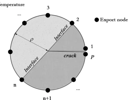
In this section, an analytical singular element for steady-state thermal conduction problem of bimaterial crack is constructed as shown in Fig.2. The interior fields of proposed element are described by using the analytical symplectic eigen solutions, hence it is termed as the “symplectic analytical singular element (SASE)”. Taking advantages of the proposed SASE, numerical solution of GFIFs can be solved. The present singular element with radius ρ is connected with the surrounding conventional elements through the "export nodes" which are evenly distributed on the element's circumference as shown in Fig.2. The node indexes are arranged from 1 to P as illustrated in Fig.2, and the number of nodes is not limited to a specific value, more export nodes will benefit the solving accuracy.

Choosing the first finite expanding terms (here we choose the first P terms) from Eq.(19) as trial functions:

( )

* ( ) ( )

1

j

P _{j j}

T j

T eξµ

γ

ψ

=

=

∑

, S_r* P_{j 1} ( )jeξµ( )j _r( )j

γ

ψ

=

=

∑

(33)

The superscript "*_{" represents trial function to distinguish from full eigen expansion Eq.(19). In this}

way the unselected expanding terms in Eq.(19) are ignored and will introduce error as a result. But when sufficient expanding terms are selected the resulted error can be limited. Rewrite the trial functions in the form of matrix gives:

* T T

T = f A

γ

, S_r* = f A_rT

γ

(34)

where

[

(1)

,

(2)

,...

( ) TP

]

γ

γ

γ

=

(0) (1) (2) diag(eξµ ,eξµ ,eξµ ...)

=

A (35)

(1) (2) ( ) T

[ , ,... P ]

T =

ψ

T

ψ

T

ψ

T

f , [ (1), (2),... ( ) TP ]

r =

ψ

r

ψ

r

ψ

r

f (36)

Substituting the i-th export node's coordinates ( , )

ρ θ

_i (Noted here that the angular coordinate θi should

be considered in the sub-coordinate system) into the above expressions, the nodal temperature vector

T 1 2

[ , ,... ]T T T_P

=

t can be specified by

t = LB

γ

(37)

where (1) ( 2) (3)

diag( µ , µ , µ ...)

ρ ρ ρ

=

B and L is the transform matrix specified by

(1) (2) ( )

1 1 1

(1) (2) ( )

2 2 2

(1) (2) ( )

( ), ( ),... ( ) ( ), ( ),... ( )

...

( ), ( ),... ( ) P

T T T

P

T T T

P

T N T N T N

ψ θ ψ θ ψ θ

ψ θ ψ θ ψ θ

ψ θ ψ θ ψ θ

⎡ ⎤ ⎢ ⎥ ⎢ ⎥ = ⎢ ⎥ ⎢ ⎥ ⎣ ⎦ L (38)

The unknown expanding coefficients can be expressed by the nodal temperature as

1 1

− −

=

B L t

γ

(39)

Hence the interior fields can be expressed by using the nodal temperature as

* T 1 1

T

T − −

= f AB L t, Sr*= f AB L trT −1 −1 (40)

The above formulas can be generally recognized as the “shape functions” in the frame of FEM although they are not standard polynomial forms of FEM shape functions. Substituting the above trail functions into the variational principle Eq.(11) and consider that the trial functions satisfy the requirements of fundamental equations in the discussed domain and homogeneous boundary conditions on the crack surfaces, the variational principle can be simplified into

{

* *

}

0 ( ) 3

1 ln

δ i i d 0

r C

i T S

α

ξ ρ θ

=

∫

⎡⎣ ⎤⎦ = =

∑

(41)

Taking advantage of the above variational principle, the stiffness matrix can thus be derived and specified by

(

3 ( )

)

T T 1

1 0 d

i Ci

T r i α θ − − =

∑ ∫

K = L f f L (42)

Notice that the integration domain for each material is from 0 to αi in the sub coordinate system

OC

i i

θ

.

6. Discussion

The calculation method of GFIFs and the integration of the proposed SASE should be discussed separately. According to Eq. (42), it can be found that the integration for the proposed 2D circular element is done over its circumference (which is a 1D domain), and this feature of the proposed SASE simplifies the integration procedures compared with conventional 2D elements. Furthermore, since all

the components in fT and fr are given explicitly, the integration can be done analytically without any

difficulty.

After solving global equation of the FEM system, the nodal temperature can be solved, and then the GFIFs can be solved directly by Eq.(39). Hence, the complex post-processing is unnecessary in the present method.

7. Modelling

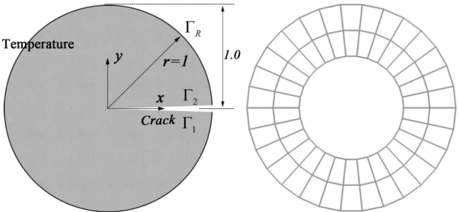
Cracked disc: Consider a unit disc as well as the FE mesh as shown in Fig.3. The boundary conditions on the lower crack surface Γ1 and upper surface Γ2 are specified by

1 2

0, on ,

/

0, on

T

=

Γ

∂

T

∂

θ

=

Γ

(43)

And the boundary condition on the circular portion ΓR of the disc is specified by

/

, on

_R

T r y

∂

∂

=

Γ

(44)

In the FE mesh, the crack tip area is occupied by the proposed SASE while the other areas are meshed by using conventional isoparametric bilinear elements. The characteristic equation of symplectic eigenvalue for the present problem can be obtained from Eq.(27), and the eigenvalues can be solved

analytically and specified by

µ

=

(2

n

−

1) / 4,

n

=

1,2,3,...

. The approximate solution for this steady-state

thermal conduction is specified by[12]:

1/4 3/4 5/4 7/4

( , )

1.35812

sin( / 4) 0.970087

sin(3 / 4) 0.452707

sin(5 / 4)

(

)

T r

θ

=

−

r

θ

+

r

θ

−

r

θ

+

O r

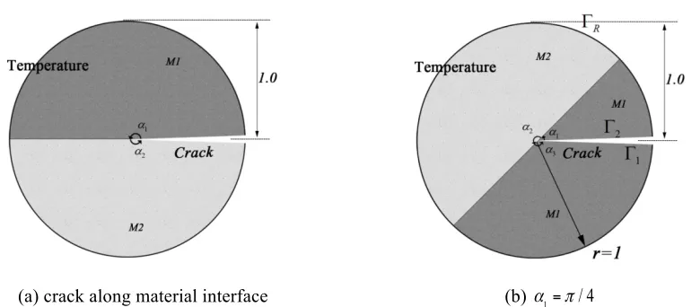
(45)

Bimaterial cracked disc: Consider a cracked disc which is composed of two different materials as shown in Fig.5. Specially, the bimaterial crack locates along the material interface is also considered. The boundary conditions are kept the same as the above single material cracked disc. The thermal

conductivities are

k k

₁

/

₂

=

1/ 2

and the vertex angles satisfyα2=π, α α1+ 3=π.

For the special case shown in Fig.5(a) the eigenvalues can be obtained by solving the characteristic equation Eq.(27) which, for this special case, can be solved analytically and the eigenvalues are

specified by

µ =

arctan(

±

k k

₁

/ )

₂ . The present results of GFIFs of the case shown in Fig.5(a) obtained

by using different numbers of export nodes of SASE are listed in Tab.2. While for a general case where

1 /4

α π= , the symplectic eigenvalues should be obtained by solving the characteristic equation Eq.(27)

numerically, and the first few numerical results of the symplectic eigenvalues are listed in Tab.3. The explicit expressions of the corresponding eigenvectors can be obtained by substituting the symplectic eigenvalues into Eq.(28)-(30). The present results of GFIFs obtained by using different numbers of export nodes of the SASE are listed in Tab.4. The predictions listed in Tab.2 and Tab.4 also provide a convergence study on the number of the SASE's export node which is of crucial importance in practical usage. In view of the obtained results, it is found that with the increase of the export nodes, the numerical predictions trend to converge. And for all the discussed cases, it is observed that 31 export nodes are sufficient enough to obtain excellent solving accuracy.

The contours of heat flux densities around the crack tip with unit k₁ are shown in Fig.6 and Fig.7,

respectively. It is interesting to find that q_θ is continuing over the domain but q_r is not. Besides, the

value of q_θ on the lower crack surface are zero. According to these numerical results, it can be found

that the present method strictly satisfy the requirements of the compatibility conditions Eq.(3) and (4) on the material interface as well as the boundary condition on the crack surfaces. In addition, thanks to the advantages of the proposed SASE, the predictions around crack tip fields are very accurate.

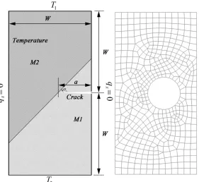
Bimaterial inclined edge crack: Consider W×2W bimaterial rectangular plate containing an edge

crack as shown in Fig.8. The lower surface of the crack is insulated while the temperature on the upper surface of the crack is zero. The left and right sides of the plate are also insulated. The temperatures on

the lower and upper sides of the plate are T₁ and T₂, respectively. The sketch of the plate as well as the

symplectic eigenvalues are listed in Tab.3. In this example o 1 100 C

T = is chosen and the numerical

results of GFIFs with the variation of T₂ are listed in Tab.5. It is observed that the values of

γ

₁,

γ

₃,

4

γ

and

γ

₅ increase monotonically with T₂, while the values of

γ

₂ decrease with T₂.

8.Conclusion

The steady-state thermal conduction with singularities resulted from inclined cracks terminate at the material interface in composite structures is investigated systematically. By using the symplectic dual approach, the analytical symplectic eigenvalues are obtained, explicit forms of the symplectic eigen solutions are specified. Then, a novel symplectic analytical singular element (SASE) is constructed based on the obtained symplectic eigen solution. The interior fields of the proposed SASE are accurately described by the higher order symplectic eigen solutions, therefore the generalized flux intensity factors (GFIFs) can be solved with highly solving accuracy. According to the numerical results, it is shown that the solving accuracy of the present method is satisfactory when 17 export nodes are used. And when 31 export nodes are used the relative errors are negligible. In addition, the GFIFs can be solved directly without any prost-processing. The present method can be further extended for the thermal conduction problem in anisotropic materials, and it will be reported in the future.

9. Acknowledgements

The supports of the National Natural Science Foundation of China (No.11502045, and No. 11372065), the Fundamental Research Funds for the Central Universities (DUT15RC(3)029) are gratefully acknowledged.

10. Reference

[1]. MF. Pernice, NV. de Carvalho, JG. Ratcliffe, SR, Hallett. Experimental study on delamination migration in composite laminates. Composites Part A, vol. 73, pp. 20-34, 2015.

[2]. GC. Sih, Heat conduction in the infinite medium with lines of discontinuities, Journal of Heat Transfer, vol. 87, pp. 293-298, 1965

[3]. AY. Kuo, Interface crack between two dissimilar half spaces subjected to a uniform heat flow at infinity-open crack, Journal of Applied Mechanics, vol. 57, pp. 359-364, 1990

[5]. CK. Chao, LY. Kuo, Thermal problem of curvilinear cracks in bonded dissimilar materials with a point heat source, International Journal of Heat and Mass Transfer, vol. 36, pp. 4085-4093, 1993

[6]. L. Marin, An invariant method of fundamental solutions for two-dimensional steady-state anisotropic heat conduction

problems, International Journal of Heat and Mass Transfer, vol. 94, pp. 449-464, 2016

[7]. N. Hasebe, S. Kato. Solution of a bonded bimaterial problem of two interfaces subjected to different temperatures, Archive of Applied Mechanics, vol. 86, pp. 445-464, 2016

[8]. L. Jing, DS. Yang, Virtual Boundary Meshless with Trefftz Method for the Steady-State Heat Conduction Crack Problem, Numerical Heat Transfer, Part B: Fundamentals, vol. 68, pp. 141-157, 2015

[9]. ZH. Zhou, CH. Xu, XS. Xu, AYT. Leung, Finite-Element discretized symplectic method for steady-state heat conduction with singularities in composite structures, Numerical Heat Transfer, Part B: Fundamentals, vol. 67, pp. 302-319, 2015

[10]. Z. Yosibash, B. Szabo, Numerical analysis of singularities in two dimensions Part 1: Computation of Eigenpairs,

International Journal of Numerical Methods for Engineering, vol. 38, pp 2055–2082, 1995.

[11]. N. Omer, Z. Yosibash, M. Costabel, M. Dauge. Edge flux intensity functions in polyhedral domains and their extraction

by a quasidual function method, International Journal of Fracture, vol. 29, pp 97–130, 2004.

[12]. Z. Yosibash. Singularities in elliptic boundary value problems and elasticity and their connection with failure initiation,

pp. 73-96, Springer, 2012.

[13]. S. Shannon, Z. Yosibash, M. Dauge, M. Costabel. Extracting generalized edge flux intensity functions with the

quasidual function method along circular 3-D edges, International Journal of Fracture, vol. 181, pp. 25–50, 2013.

[14]. J. Yvonnet, QC. He, QZ. Zhu, JF. Shao, A general and efficient computational procedure for modelling the Kapitza

thermal resistance based on XFEM, Computational Materials Science, vol. 50, pp. 1220-1224, 2011.

[15]. WA. Yao, WX. Zhong, CW. Lim. Symplectic elasticity, pp: 181-223, World scientific, Singapore, 2009.

[16]. XF. Hu, WA. Yao, A novel singular finite element on mixed-mode bimaterial interfacial cracks with arbitrary crack

surface tractions, International Journal of fracture, vol. 172, pp. 41-52, 2011.

[17]. JS. Wang, QH. Qin. Symplectic model for piezoelectric wedges and its application in analysis of electroelastic

singularities, Philosophical Magazine, vol. 87, pp. 225-251, 2007.

[18]. CH. Xu, ZH. Zhou, XS. Xu, AYT. Leung, Electroelastic singularities and intensity factors for an interface crack in

[19]. HW. Zhang, WX. Zhong. Hamiltonian principle based stress singularity analysis near crack corners of multi-material

junctions, International Journal of Solids and Structures, vol. 40, pp. 493-510, 2003.

[20]. WA. Yao, XF. Hu, A novel singular finite element of mixed-mode crack problems with arbitrary crack tractions,

Mechanics Research Communications, vol. 38, pp. 170-175, 2011.

[21]. XF. Hu, WA. Yao, A new enriched finite element for fatigue crack growth, International Journal of Fatigue, vol. 48, pp.

247-256, 2013.

[22]. WA. Yao, ZJ. Zhang, XF. Hu, A singular element for Reissner plate bending problem with V-shaped notches,

Theoretical and Applied Fracture Mechanics, vol. 74, pp. 143-156, 2014.

[23]. WA. Yao, XF. Hu, A Novel Singular Finite Element on Mixed-Mode Dugdale Model Based Crack, Journal of

Engineering Materials and Technology, vol. 134, pp. 021003, 2012.

[24]. AYT. Leung, XS. Xu, ZH. Zhou, Hamiltonian approach to analytical thermal stress intensity factors—Part 1: Thermal

Intensity Factor, Journal of Thermal Stresses, vol. 33, pp. 262-278, 2010.

[25]. AYT. Leung, XS. Xu, ZH. Zhou, Hamiltonian Approach to Analytical Thermal Stress Intensity Factors—Part 2

Tab.1 Predictions on the GFIFs of the cracked single material disc

Export Node Num.

γ

1 Err%

γ

2 Err%

γ

3 Err%

13 -1.3361763 -1.61574 0.93698025 -3.41276 -0.42601371 -5.89637

17 -1.3456556 -0.91777 0.95223888 -1.83985 -0.44502567 -1.69676

31 -1.3581286 0.00063 0.97008793 0.00009 -0.45270759 0.00013

Tab.2 GFIFs of the bimaterial cracked disc for the case α₁=0

Export Node Num.

γ

1

γ

2

γ

3

13 -1.11847290 0.66341500 -0.30219865

17 -1.12416167 0.67356153 -0.31717382

25 -1.13012358 0.68743453 -0.33165312

Tab.3 Numerical solutions of the first few symplectic eigenvalues for the case α₁=π/ 4

1

n= 2 3 4 5 6 7

Tab.4 GFIFs of the bimaterial cracked disc for the caseα₁=π/ 4

Export Node Num.

γ

₁

γ

2

γ

3

13 -7.91930310 3.00392948 -0.96284920

17 -7.94993727 3.07362578 -0.96324238

25 -7.97847336 3.06983473 -0.98373263

Tab.5 GFIFs of the bimaterial inclined edge crack

o 2( C)

T

γ

₁

γ

2

γ

3

γ

4

γ

5

0 30.424592 5.029149 0.668151 1.096963 -0.980787

40 38.654873 4.774610 2.692545 1.463760 -0.865410

80 46.885155 4.520071 4.716940 1.830557 -0.750032

120 55.115437 4.265532 6.741335 2.197354 -0.634655

160 63.345719 4.010993 8.765729 2.564151 -0.519278

Captions of figures

Fig.1 Inclined bimaterial crack and the sub-coordinate system

Fig.2 The SASE for bimaterial crack terminate at the interface

Fig.3 A cracked disc and the FE mesh with the SASE

Fig.4 Contours of heat flux densities around the crack tip

Fig.5 Bimaterial disc containing a inclined interface crack

Fig.6 Contours of heat flux densities around the bimaterial crack tip for the case α1=0

Fig.7 Contours of heat flux densities around the bimaterial crack tip for the case α1=π/4

[image:22.612.222.419.135.359.2]

[image:23.612.205.412.91.252.2]

[image:24.612.145.469.175.325.2]

[image:25.612.81.529.102.365.2]

(a) q_θ (b) q_r

[image:26.612.109.499.86.257.2]

(a) crack along material interface (b) α₁=π/ 4

[image:27.612.85.526.87.338.2]

(a) q_θ (b) q_r

[image:28.612.81.532.81.340.2]

(a) q_θ (b) q_r

[image:29.612.169.450.93.351.2]