Stenomaps: Shorthand for shapes

City, University of London Institutional Repository

Citation: Van Goethem, A., Reimer, A., Speckmann, B. and Wood, J. (2014). Stenomaps:

Shorthand for shapes. IEEE Transactions on Visualization and Computer Graphics, 20(12),

pp. 2053-2062. doi: 10.1109/TVCG.2014.2346274

This is the accepted version of the paper.

This version of the publication may differ from the final published

version.

Permanent repository link: http://openaccess.city.ac.uk/id/eprint/14151/

Link to published version: http://dx.doi.org/10.1109/TVCG.2014.2346274

Copyright and reuse: City Research Online aims to make research

outputs of City, University of London available to a wider audience.

Copyright and Moral Rights remain with the author(s) and/or copyright

holders. URLs from City Research Online may be freely distributed and

linked to.

City Research Online:

http://openaccess.city.ac.uk/

publications@city.ac.uk

Stenomaps: Shorthand for shapes

Rh ôn

e-A

lp

es

Rhôn_{e-A lp}es

L an gu ed o c -

Pro ve

nce - Po_ito u- _Lim ou s

C en

tre C_en

tr e Cen

tre

Pa

ys-d

e-la-L

oire Bo_u rg

og ne

Auve rgne

Au_v

e

rg

n e Île-de-P

i c ar d i e

Nord_-Pas

Midi-_{éné Pyr}

es

Midi-én Pyr ées Lo rra ine Fr an ch e C h am p ag_ne -A ls a c e H a u t e B a s s

e

A

q

ui t

a in

e B

r e_{t a g n e}

C o r s e de Calais N o rm an die N orma_ndie France A r d e n n_e -C o m té Ch_ar en te R o_u ss ill o n

A l p

es

-

Côte d

’Azu

r

Abstract— We address some of the challenges in representing spatial data with a novel form of geometric abstraction – the stenomap. The stenomap comprises a series of smoothly curving linear glyphs that each represent both the boundary and the area of a

poly-gon. We present an efficient algorithm to automatically generate these open,C1_{-continuous splines from a set of input polygons.}

Feature points of the input polygons are detected using the medial axis to maintain important shape properties. We use dynamic programming to compute a planar non-intersecting spline representing each polygon’s base shape. The results are stylised glyphs whose appearance may be parameterised and that offer new possibilities in the ‘cartographic design space’. We compare our glyphs with existing forms of geometric schematisation and discuss their relative merits and shortcomings. We describe several use cases including the depiction of uncertain model data in the form of hurricane track forecasting; minimal ink thematic mapping; and the depiction of continuous statistical data.

Index Terms—Schematisation, Maps, Algorithm, Design

1 INTRODUCTION

Generalisation and abstraction are fundamental processes in the con-struction of cartographic views of data. These can range from straight-forward geometric simplification processes that attempt to reduce data volumes without significantly affecting visual appearance to more complex abstractions where referents are more radically transformed into their symbolic representations. The need for higher levels of ab-straction may be greater when combined with thematic and other data in an information visualization context with its demand for graphi-cal space and distinct visual variables. Schematisations that preserve topological relationships at the expense of geometric fidelity or car-tograms that generate data-centric reprojections of space add to a range of design options available for those wishing to visualize geospatial data. This paper offers a further extension of that design space by providing a new method of transforming two-dimensional polygonal representations into smoothly curving one-dimensional linear features

orglyphs. This form of extreme geometric abstraction we term the

stenomap, from the Greekstenosmeaning ‘narrow’ and a direct

anal-ogy with stenography – the transformation of letter form into short-hand symbols. The approach is inspired in part by some of the work

• Arthur van Goethem and Bettina Speckmann are with TU Eindhoven.

E-mail:[a.i.v.goethem|b.speckmann]@tue.nl

• Andreas Reimer is with Universit¨at Heidelberg.

E-mail: andreas.reimer@geog.uni-heidelberg.de

• Jo Wood is with City University London. E-mail: j.d.wood@city.ac.uk

Manuscript received 31 March 2013; accepted 1 August 2013; posted online 13 October 2013; mailed on 4 October 2013.

For information on obtaining reprints of this article, please send e-mail to: tvcg@computer.org.

of the 20th century cubist and abstract expressionist artists, including Picasso and Pollock, who explored radical transformations of the de-piction of form that were still able to capture something of its essence. We provide several arguments for considering area-to-line transfor-mations. Fig. 1 displays an ordered sequence of transformations of a polygon increasing in their abstraction. While generalising polygon boundaries is common (Fig. 1(b)), and often valuable, it is constrained by the topological arrangement of adjacent polygonal units along com-mon boundaries. Transformation to a zero-dimensional point feature (Fig. 1(e)) frees up graphical space, however, topological relationships and most geographic context is lost in the process. Transformation to a linear representation offers the opportunity to free up graphical space while maintaining a sense of the form and arrangement of the original feature. Area-to-line transformation is most commonly achieved via medial axis generation (Fig. 1(c)), but while useful as an intermediate step for shape characterisation it has limited cartographic value and may be confused with genuine linear features such as river or road networks. The more smoothly curved stenomap glyphs (Fig. 1(d)) capture something of the form of the polygon boundary while being independent of adjacent polygon geometry and freeing up graphical space for other representations. We describe how stenomaps may be created algorithmically and explore the potential for such representa-tions to open up the design space for the depiction of uncertainty, in thematic mapping and interaction with other visual variables.

Organization.We first discuss the design choices for the glyphs used

Fig. 1. Increasing the abstraction of France. From left to right: (a) un-transformed polygon, (b) curved schematization, (c) pruned medial axis, (d) stenomap glyph, (e) dot.

types of glyphs computed (Section 5) and we describe user-parameters that help explore the possibility-space. We discuss several use-cases (Section 6) to explore the role that stenomap abstraction can have in the depiction of geospatial data. Finally, we conclude with a discus-sion and possible directions for future work (Section 7).

Background.The representation of outlines has received significant

attention within the field of cartography. Both straight-line and curve schematisation, as well as simplification, have been well studied. Well known results in cartographic generalisation such as linear simplifi-cation (e.g., [14, 20, 39]) maximise the information maintained when reducing the level of detail. Automated cartographic generalisation (for foundational terms and state of the art see, [12, 24, 11]) is driven by intricate knowledge of the target scale or Level of Detail of the map product (e.g., [9]). By contrast, the focus of schematisation is to minimise detail while maximising task-appropriateness of the visual-isation [23]. Straight-line schematvisual-isations (e.g., [5, 10]) have mainly focussed on orientation-restricted representations. Similarly, curved schematisation (e.g., [17]) has focussed on fixing the type of curve.

Representing shapes using curves has also been considered in other research fields, such as computing tangent-continuous paths for

cut-ting tools (e.g., [15, 19]). Miet al.[27] take an alternative approach,

deconstructing a shape into parts to find the required abstraction. B´ezier curves, first described in 1959 [13], are a family of smooth curves described by a set of control points. As the control points define the tangents at the end points of the curve, B´ezier curves can be used

to createC1_{- orC}2_{-continuous splines. Fitting a B´ezier spline to a}

polygonal line can not be optimized in closed form, however iterative algorithms exist (e.g., [26, 32]). Stone and DeRose [36] show how to determine the existence of self-intersections in a cubic B´ezier curve.

The medial axis, introduced by Blum [8], is a way to describe the skeleton of a polygon. As the medial axis is not stable under small transformations, various pruning algorithms have been proposed [2, 3, 6, 34]. Only maintaining the parts describing the main features of the polygon gives rises to a more stable version of the medial axis. In computer vision, shock graphs have recently gained considerable attention as this extended structure built on top of the medial axis can be used for automated shape recognition (e.g., [25, 38]).

Space-filling curves are regularly structured curves that fully cover

an-dimensional space. These curves can be seen as “[mapping] a

one-dimensional space onto a higher-dimensional space.” [40]. Re-cently, the use of space-filling curves to display hierarchical or com-plex datasets has gained attention (e.g., [1, 37]). In contrast to space-filling curves, our approach focusses on a curve that covers only a part of the area while still sufficiently describing it.

(b) (c)

(a) (d)

Fig. 2. Representing Spain as a glyph. (a) Polygon and (pruned) medial axis. (b) Border representation. (c) Collapse to medial axis. (d) Trade-off between border and area.

(c) (a)

(d) (b)

P0

v w

b P

w

v b

Fig. 3. (a) Four maximally inscribed circles. The center points of all maximally inscribed circles form the medial axis (red). (b) Reducing

the radius of all maximally inscribed circles negatively offsetsP. (c) An

end-branchbwith parentwand leafv. (d) Area contributed by the

end-branchb.

2 DESIGN CHOICES

Reducing a polygon to a line inevitably reduces its expressiveness. Hence, if we desire such an abstraction, careful thought should go into the formation of this line. In this section we discuss the design choices made when developing stenomaps.

C1_{-continuous. The glyphs we create are (along single strokes)C}1

-continuous. The continuity of the curve gives a hand-drawn appear-ance stimulating the perceived inexactness of the geometry. Using smooth swipe-like, near casual representations promotes an attention shift to the actual data, further emphasizing the imprecision in the

ge-ometry. For a discussion onCx_{-continuity see Section 3.}

Complexity. All glyphs should be presented using as few curves

as possible. The curves should sufficiently describe the polygon at hand, but no excess information should be provided. We target our stenomaps at data not tied to an exact location. As exact geographic information is unimportant and excess information reduces the effi-ciency of the map, glyphs should have the lowest possible complexity. All attention should be focussed on the main data presented.

Area and boundary. Representing a polygon by a linear smooth

glyph reduces the expressive power compared to the original two-dimensional polygon. Whereas a polygon implicitly describes both the area and the boundary, this is less clear for an open curve. In the case of elongated polygons both area and boundary representation give overlapping requirements. A curve following the “central axis” suitably describes both. For compact polygons, however, the require-ments contradict (see Fig. 2). A partial boundary representation lacks the implied volume of the polygon, whereas a “central axis” is unable to properly represent the shape of the polygon. We note that a trade-off exists between representing the boundary and the area. We require the maximum minimum distance to the curve to be optimized while also sufficiently representing the boundary.

3 TECHNICALPRELIMINARIES

Medial axis.Themedial axis transformwas first introduced by Blum

[8] and is defined for a polygonPas the closure of the set of points

with two or more closest points located on the boundary ofP. This set

is usually simply referred to as themedial axisand is a subset of the

edges implied by the edge-based Voronoi diagram [4]. The medial axis

is a unique description of the shape ofP. Each point on the medial axis

is associated with a maximally inscribed circle ofP(see Fig. 3(a)) and

the union of all circles fully coversP. More specifically, there is a

representation makes it easy to compute offset polygons by changing

the radius of all inscribed circles by a fixed constantc(see Fig. 3(b)). A

negative offset (essentially shrinking the polygon) can result in several

connected components. Maintaining a minimum circle radius ofr 0

prevents such fragmentation.

Our input is a simply connected polygonP. (Note, though, that

our algorithms could easily be extended to polygons with holes.) The

medial axisMof a simply connected polygon is a tree. Aleaf ofM

is a vertex of degree one and is located on the boundary of the input

polygon. Anend-branch bis a maximal sequence of edges connected

via vertices of degree two, where at least one of the two end points is a vertex of degree one (see Fig. 3(c)). An end-branch has two end

points, one of which is a leaf, the other is aparent(which could

si-multaneously also be a leaf). An end-branchbisprunedby removing

all of the edges and degree one and two vertices ofbfrom the medial

axis. If we reconstruct the polygon belonging to the pruned medial

axis we obtain a locally smoothed polygonP0_{. Thecontributed area}

of an end-branch is the area ofP P0_{(see Fig. 3(d)). A pruned medial}

axis can be used for a variety of purposes and hence there exists a sig-nificant amount of literature which discusses various pruning measures and methods [2, 6, 29, 33, 34].

Visibility graphs. Given a set of pointsS, the visibility graph is the

union of all edges between any pair of points inSthat can see each

other. We use a specific instance of the visibility graph where visibility

is defined by the polygonPand the setSconsists of all vertices ofP.

Two points can see each other if the straight-line connection between

them is fully contained in the interior or the boundary ofP. We use

this visibility graph to compute shortest Euclidean paths inP.

B´ezier splines.A cubic B´ezier curve can be fit “optimally” to a given

polygonal line using iterative Newton-Raphson approximation [32].

Similarly, with the help ofdynamic programming, a series of cubic

B´ezier curves can be fit optimally to a polygonal line or a polygon [17]. Splines (the concatenations of B´ezier curves) can have different

de-grees of continuity. A spline isCx_{-continuous if the derivative of}

de-greexof the spline exists and is a continuous function. When a B´ezier

spline isC1_{-continuous (smooth), the control points of consecutive}

curves line up (see Fig. 4(a)). Consequently, fitting curves to differ-ent parts of the polygonal line is no longer independdiffer-ent and, therefore, dynamic programming can not guarantee an optimal solution. If we re-duce the allowed solution space, by fixing the required tangents at all vertices, the fitting of different curves is independent once more. We require the tangents at each vertex to be perpendicular to the bisector (see Fig. 4(b)). The start- and end-vertex have no well defined tan-gents, but no continuity is required here either. While fixing tangents beforehand is not required to compute a smooth spline, if tangents are

not fixed, computing anoptimalseries of curves is hard.

4 ALGORITHM

We describe an algorithm to compute a linear,C1_{-continuous glyph}

Grepresenting a simple input polygonP. Depending on the desired

design, different types of glyphs can be generated (see Section 5). Our algorithm consists of four distinct steps. First, we detect feature

points that define the characteristic shape ofP. Second, we compute

the region in which the glyph should be located. Third, we determine

the base shape of the glyph by finding a polygonal line (thebackbone)

that represents the polygon well. The shape of the backbone deter-mines the shape of the final glyph to a large degree. Hence we describe

↵ ↵

(a) (b)

Fig. 4. (a)C1_{-continuous curves have a continuous derivative. The}

con-trol points of consecutive curves line up. (b) Fixing the required tangent beforehand allows for a dynamic programming solution.

Algorithm 1ComputeGlyph(P)

Require: Pis a simple polygon

Ensure: Gis a glyph ofP, strictly positioned insideP

{Find feature points}

1: Create the medial axisMofP

2: PruneMto obtain feature points ofP

{Obtain glyph region}

3: Trim branches ofM

4: SimplifyPbased onM

{Find backbone}

5: Compute all paths between feature points

6: Find the backboneBvisiting all feature points

{Create glyph}

7: Fit a smooth spline toBto obtain glyphG

two different approaches which result in radically different backbones. In the final step we fit a cubic B´ezier spline to the backbone. Again, there are several possibilities, resulting in different types of glyphs. If the input is planar, our algorithm can be run in parallel on all polygons. See Algorithm 1 for a summary. We explain all steps in detail below.

4.1 Feature points

To maintain the characteristic shape of the input polygonP, we first

detect the mainfeature points. We take a geometric point of view

and use the pruned medial axis for feature recognition. Our method is based on the work by Bai and Latecki [2], who use area as a measure to guide the pruning. Area is relatively outlier- and noise-insensitive and is also used as a measure in cartographic simplification [39], making it suitable for our purposes.

The method by Bai and Latecki computes for each end-branch the

size of the area that it contributes toP. By repeatedly pruning the

end-branch that contributes the least amount of area toPthe medial axis

can be reduced to its main features. The algorithm by Bai and Latecki compares area loss to the previous, already reduced, incarnation of the polygon. As a consequence it may reduce large subtrees by iteratively removing small sections of the area. To prevent important features from being pruned prematurely we maintain the total area that has been pruned in each subtree. We maintain this information in the leaves and parent nodes and update it in amortized constant time when pruning an end-branch. Each edge is pruned only once and we can compute the

area lost inO(n)time, so the total pruning process takesO(n2_)time.

The leaves of the pruned medial axis correspond to the main features. When displaying a subdivision (e.g., countries in Europe) we typ-ically desire a similar complexity level across the map. To achieve this we admit only pruning steps that remove subtrees of a given max-imum size. That is, any single prune action is not allowed to remove a branch representing a subtree larger than a user-specified percentage of the average polygon area in the map. The pruning process stops when this constraint is violated or when only a single path is left.

As discussed in Section 2, elongated polygons and compact poly-gons require a different level of detail. To facilitate this we introduce an extra factor measuring the compactness of a polygon. Specifically, we use the squared length of the longest path in the medial axis di-vided by the area of the polygon as a size independent description of compactness (see Fig. 5). Any measure using boundary length instead

(a) (b)

P0 _P

(c) P

P00

Fig. 6. (a) A regular offset may cause branches to collapse and

discon-nect the polygon. (b) The offset polygonP0_{defines the space for the}

glyph. (c) The (possibly degenerate) polygonP00_{for the backbone.}

of the longest path in the medial axis would be more sensitive to local noise. The local area loss accepted in a single prune action is limited

by: 0.25⇤a⇤avgArea⇤longestPath2_{/polygonArea, where 0a1}

is a user-defined parameter.

4.2 Regions

We now compute the regionP0_{within which the glyph is contained. To}

make the glyphs clearly distinguishable we require them to be located strictly within the polygon they represent. Where possible a minimum distance to the boundary of the polygon is guaranteed. Using a modi-fied offset operator ensures that a minimum area is maintained within which the glyph can be fit. A regular offset can cause the polygon to become disconnected and may collapse entire branches (see Fig. 6(a)). The modified offset operator uses the the radius information stored in the medial axis. We first retract all end-branches of the medial axis by a given percentage (we use 30%). That is, we measure the length of the end-branch and starting at the leaf vertex remove all vertices and edges until the summed length of the removed edges equals 30% of the original end-branch length. If the next edge induces a percentage larger than 30% we shorten that edge and introduce a new leaf vertex. Now we apply a modified negative offset to the radii stored for the inscribed circles of the medial axis. We reduce the radii of all inscribed circles by a constant – as in a regular offset – unless this forces a ra-dius to drop below a given threshold. In this case we set the rara-dius to the threshold to prevent a collapse of the polygon (inscribed cir-cles with an initial radius smaller than the threshold are simply main-tained). Using a strictly positive threshold ensures a single connected polygon, using a threshold of zero can result in a degenerate polygon. The union of all reduced circles uniquely describes the negatively off-set polygon. It can be computed in a single traversal of the medial axis. Our offset does not retract end-branches as all circles are maintained.

The regionP0_{for the glyph is a negatively offset polygon with a}

strictly positive minimum radius (Fig. 6(b)) to ensure that the curve can turn without intersecting itself or the boundary. Inside the region

P0_{we compute a second offset polygonP}00_{(Fig. 6(c)) in which the}

backboneof the glyph is located (see Section 4.3). When the backbone

is turned into a smooth glyph we require some additional space for smoothing and hence the backbone needs to lie in a strictly smaller region than the region of the glyph. Here we do not require a strictly

positive minimum radius and, hence,P00_{may be degenerate.}

f4

f1

f2

f3

P00

Fig. 7. Consecutive feature points (e.g., f4, f1) are connected by a

boundary path. Other pairs (e.g., f1, f3) are connected by the

short-est Euclidean path insideP00_.

4.3 Backbone

Abackboneis a planar straight-line graph that visits all feature points

and describes the polygon well. We consider two types of backbones: simple paths and trees. Backbones are polygonal representations of the glyphs and are used as base shape for the final glyphs (see Section 5).

Path-backbone. Our input is the offset polygonP00_{and the feature}

points cyclically ordered aroundP(see Fig. 7). We aim to find a good

simple polygonal path visiting all feature points which stays inside or

on the boundary ofP00_{. To do so we first connect any pair of feature}

points with a path. This paths follows the boundary ofP00_{if it connects}

two consecutive feature points. For all other pairs we compute the

shortest Euclidean path insideP00_{using the visibility graph [4].}

As discussed in Section 2 the final glyph, and thus the backbone, should represent both area and boundary of the polygon. We represent this dual requirement by a linear trade-off between the percentage of boundary covered and the maximum distance to the curve from any

point in the polygon. Letsboundaryandsareabe the boundary and area

score respectively and 0b1 a user-set parameter. The score of

the backbone is defined as(1.0 b)⇤sboundary+b⇤sarea.

The boundary scoresboundaryrepresent the percentage of the

bound-ary of the original polygon that is covered by an offset of the backbone.

Similarly, the area-scoresareais the maximum minimum distance to

the backbone as a percentage of the maximum minimum distance to the polygon boundary (see Fig. 8). As an approximation of the maxi-mum minimaxi-mum distance we take the maximaxi-mum minimaxi-mum distance of any point on the medial axis to the backbone.

Given the computed paths between any pair of feature points and the described weighing scheme, we find the optimal, simple path visiting all feature points. Finding such a path is NP-hard, but as the number of feature points is very small we can use a brute-force approach.

As the backbone is computed using a scoring function we can in-troduce additional factors to influence the result. For example, our framework implements a penalty function to prevent duplicating parts of the path as well as a sea- or map-border preference. Ensuring the boundary of a map is covered may be preferential if the shape of the subdivision is familiar, but separate polygons are less recognizable. All the figures presented in this paper were, however, created without the use of these additional parameters.

Tree-backbone. Path-based glyphs achieve a high level of

abstrac-tion. Sometimes a more complex structure may be desirable that bet-ter captures the shape and the area of the polygon. We also consider backbones based on trees. Tree-backbones are computed directly from

the offset polygonP0_{. We turn the boundary ofP}0_{into an undirected}

graph and detect cycles using depth-first search. Cycles are opened by disconnecting and shortening one of the edges in a cycle.

4.4 Glyphs

The backbone is a concise and abstract representation of the input polygon. In the final step we polish the appearance of the backbone

using smooth,C1_{-continuous curves. As the essential shape is already}

determined by the backbone there is a large degree of artistic freedom in this last step. Several types of glyphs can be created, possibly de-signed to fit the application at hand. In the next section we describe three possible glyphs that are implemented within our framework.

(a) (b)

Fig. 9. Example of simple glyphs. Outlines are supplied for reference.

5 GLYPHTYPES

Different glyphs can be fit onto a backbone and here we discuss three options.

5.1 Simple

We fit a simple, C1_{-continuous, cubic B´ezier spline to a}

path-backbone. The simplicity of the design makes this glyph most suit-able for cartographic applications. To keep the complexity of the final glyph low, we minimize the number of B´ezier curves (see Fig. 9).

The overall spline should use as few curves as possible while

stay-ing within a given error-bounderrmax. For each single curvec

rep-resenting a polygonal linep, we define its errorecas the maximum

minimum distance betweencandp. The error of a set of curvesC

ismaxc2C(ec). We use dynamic programming to minimize the

num-ber of B´ezier curves used to represent the polygonal line while staying within the error-bound [17].

There may be many different splines, using the minimum amount of curves, that stay within the given error-bound of the polygonal line. Therefore, as a secondary objective function for the dynamic program,

we compute the average distancedcof a curve to the polygonal line.

To this end, we compute the average of the squared distances between regularly sampled points along the polygonal line and the curve.

We define the costcof a curve as 1+dc/(n⇤err2_{max), wherenis}

the number of vertices of the polygonal line. As each allowed curve

has an error of at mosterrmax, the average squared distancedcis at

mosterr_max2 _{. The number of curves used to represent the polygonal}

line can never exceedn 1, hence the total cost implied by the fit of

the used curves can never exceed one. As a consequence, the result has the minimum number of B´ezier curves and has, for all solutions with this number of B´ezier curves, the curves with on average the best fit. To prevent curve intersections and self-intersections we set the cost

c=•if an intersection occurs.

5.2 Locally intersecting

As an alternative to simple,C1_{-continuous cubic B´ezier splines we let}

ourselves be inspired by the work of Picasso (“One-Liners”) [30]. We forgo smooth transitions between consecutive curves and instead

cre-Fig. 10. Example of locally intersecting glyphs.

Fig. 11. Example of tree-based glyphs.

ate an appearance of smooth behavior by connecting two consecutive

B´ezier splines with an additionalswirl(see Fig. 10).

We again use a dynamic program to find the optimal set of fitted B´ezier curves. As there is no dependency between consecutive curves, we do not need to fix tangents at the vertices beforehand. For any two

consecutive curves connecting at a vertexv, we compute the distance

dvPfromvto the polygonP. We then create an additional cubic B´ezier

curve (the swirl) whose start- and end-tangents meet up with the pre-vious and next B´ezier curve, respectively. To ensure that the swirl is fully located in the polygon the second and third control points of the

curve are positioned at a distance 0.75⇤dvPfrom the first respectively

fourth control point. We again disallow intersecting curves. In some cases swirls may be undesirable. When curves meet at a

too shallow or too sharp angle a swirl may look unnatural and aC1

-continuous connection would be preferred. LetCandDbe two

con-secutive curves connected at a vertexv. LettCandtDbe the tangents

ofCrespectivelyDatv. We defineaas the minimal angle between

tC andtD. We only add a swirl ifp/6a5p/6. Otherwise, we

forceCandDto beC1_{-continuous. This creates an interdependency}

between subproblems and, hence, we cannot claim that the dynamic programm computes the optimal solution. In practice, however, the results are quite satisfactory.

5.3 Tree-based

The final alternative are glyphs based on tree-backbones. Such glyphs can describe area more concisely, but they are also more complex than glyphs based on path-backbones (see Fig. 11).

Our input is a tree-backboneB. We say that the leaf of the longest

end-branch is therootofB. In case thatBhas only two leaves, the

root is the top leftmost leaf. Let theturning angle te,fbetween two

edgese,f on a pathpbe defined asp angle(e,f)ifeand f have

a common vertex and 0 otherwise. The turning angletpof a pathp

isÂe,f2pte,f. LetPbe the set of paths of minimum size that cover

B, where all paths p2Pgo strictly down in the tree andÂp2Ptpis

minimized. For each pathp2Pwe fit a cubic B´ezier spline using

the edge-based Voronoi diagram to ensure different splines do not in-tersect [17]. Different splines might not connect at endpoints. We extend splines using a straight line matching the end-tangent to ensure all splines are connected.

6 CARTOGRAPHIC APPLICATIONS

We first in Section 6.1 present a formal discussion on the relation of stenomaps to the existing cartographic design space. Section 6.2 to 6.4 explore three use cases for stenomaps.

6.1 Stenomaps as thematic maps

less fixed by geographic coordinates. Any information beyond

geom-etry (thematicelevation) must be expressed by encodings using the

remaining visual variables known asretinal variablesor color-pattern

variables. The retinal variables are shape, orientation, color, texture, value, size. Each has a maximum in the structural equivalence of the scale level it can express, further limited by the geometric primitive

(point, line or area, i.e.,implantation) it is applied to. The levels of

organizations are Association or Disassociation, Selection, Order and Quantity. The Length of a given variable is different for each implan-tation. Length denotes the number of possible variations that can be used while still allowing selective perception. Bertin discusses each retinal variable and its potential Length thoroughly and with many ex-amples, including special cases and precise instructions on maximiz-ing differentiation. The effects on expressiveness when usmaximiz-ing multiple retinal variable encodings simultaneously were discussed by [35]. For a discussion of the concept of Disassociation and its effects see [31]. More encyclopedic taxonomies of the actually realised design space were proposed by [16] or [21] for example, which form the baseline of more current works like [22].

The classic space of possible and realised cartographic visualisa-tions [16, 22] divides the topological structure into discrete and con-tinuous phenomena, further subdividing the discrete phenomena into points, lines and areas. Hence, discrete geographic areas can be ex-pressed only by some form of polygonal subdivision. Stenomaps break that contention and show that it is possible to represent discrete areas with cartographic lines. We observe three major changes:

I boundary lines vanish II area fills vanish

III implantation change from area to line for discrete area objects from the basemap

These changes reduce the visual complexity of the map by reducing the number of control points [23] as well as the amount of “ink” used [7]. Furthermore, change I has the following immediate effects:

• actual locations of boundaries become fuzzy, limiting the

accu-racy of placement and the ability to conduct measurements in the plane

• adjacency topology becomes fuzzy

• empty bands of expected width 2·ebecome available around

dis-crete areas. Due to isthmuses (see Fig. 6) the theoretical lower

bound for width is 2·width_minpolygon, i.e. twice the minimal

dis-cernable width of polygons,=0.6mmfor b/w and=0.8mmfor

color depictions [18]. Effects of change II are:

• maximum selective length for each retinal variable, except shape

and orientation is reduced by 1 each. This decreases the degrees of freedom for choosing retinal variables by 4. The reason for this effect can be interpreteted as a function of the drawing space real estates that color, texture, value and size need to work at full efficiency.

• maximum selective length for orientation is raised from 0 to 2,

as the area implantation does not allow selective variation of ori-entation at all.

• The net change in degrees of freedom for variation of retinal

vari-ables for selective perception is thus 2.

• figure-ground separation is amplified over the whole map [7]

As the three implantations are highly selective themselves, change III frees up the area implantation for some other feature type to be added but lessens the degree of freedom for other phenomena to be depicted with cartographic lines. The gain of whitespace due to both I and II drastically increases the potential to place further map elements in a high-contrast environment. This decreases visual interaction by si-multaneous contrast and color mixing effects. Color can be chosen in-dividually for different implantations. The map in Fig. 12(left) makes use of that effect to display multiple set memberships while having full access to the color space for the point symbols and quantitative data. We can conclude that in cases where the negative consequences

of the implantation changeArea!Linesuch as fuzzy boundaries

and adjacencies are not crucial, stenomaps could be used just as well as other maps types like choropleth maps. In cases were displaying sharp administrative boundaries is detrimental to the intended mes-sage, stenomaps offer a new cartographic arrangement with improved figure-ground seperation, lower complexity, an additional layer-slot for area depictions and a band of white space around the glyphs.

€

€ €

€ €

€ _€ €

€

€

€ €

€ €

€ €

€

€

€

€ €

€ €

€ _€ €

€

€

€ €

€ €

€ €

€

€ Legend

€ outer line:

Schengen Area inner line:EU-membership non-Schengen

Schengen

member non-member

Monarchy

Republic Eurozone € 200,000 t of potato production

Unilateral usage

(a) Multi-band line symbolisation (b) Flows in cross-border whitespace (c) Isotype icons as line replacement

Île-de -P

i c a_{r d i e} Nord

-Pas C h am p

ag_ne -H

a u

t

e de

Calais

N

o

rm

an

die

France A

r

d e n

n e

(d) Labels as line replacement

Fig. 13. Design choices for stenomaps.

6.2 Use Case: Variations on Glyphs as cartographic lines

In this section, we examine the design possibilities for visual varia-tion of glyphs as cartographic lines. On a fundamental level, glyphs inherit the basic and combinatorial traits of the line implantation, a formal discussion of which we forgo. As visual shorthand for dis-crete area objects, i.e. in application in a stenomap, we provide some further exploration of design possibilities. Stenomaps do not assume the existence of a separate base map layer. Succinctly, the usual con-straints stemming from the base map that line features are limited by, do not apply. This allows a much higher degree of variation in pattern and width of the line features. One example is to create multi-band representations such as Fig. 13(a). Here, multi-set membership and even configurations of set-membership are displayed by colored repe-titions of the basic glyphs. Though there are natural limits, these are less strict than in regular maps, due to the white space gained by the area-boundary collapse. Special care must be taken not to vary the width of the glyphs too much, lest the perception as an areal subdivi-sion be dissolved. The same care must be taken regarding brightness (value) differences. Fig. 12(left) makes use of the variation of pattern as well as color. Specifically, the effect of vibration is used following the parametrisation of [7], not unlike a Moir´e-pattern, to highlight the Schengen-participants (signatories to a cross-border migration treaty) who are also EU-members. Note that the lower contrast pairings do not produce the same effect. Such use of vibration is generally not advisable for areas and presents another advantage of stenomaps. The glyphs in this figure give a strong sense of location, as can best be seen when making the comparison with the same map solely contain-ing data (see Fig. 12(right)).

Fig. 14. Energy consumption in the Regions of France 2010. Data source: Electrical Energy Statistics for France 2010, R´eseau de trans-port d’´electricit´e 2011.

While Fig. 12(left) makes uses of the space formerly occupied by boundaries by placing point symbols and quantitative information, an-other possible application is to depict cross-border flows (Fig. 13(b)). This technique is best suited for the case of planar flow graphs and can reintroduce topology information that was made imprecise by the area collapse. The Vienna Method of Pictorial Statistics (e.g., [28]), later

known asIsotype, was most often used over very sparse base maps

or on plain white paper. Stenomaps are a natural environment where Isotype icons can dwell and prosper. They can be applied like regular carto-diagrams as in Fig. 12(left) or even be used to utterly replace glyphs by repetition. The latter technique is limited in cases where the low frequency of icons starts to dissolve the individual glyph, as is exemplified by the green elements in Fig. 13(c).

As has been mentioned, stenomaps abscond from regular base maps and thus have no or very few labels. Either through aesthetic choice or informational necessity, the glyphs can be replaced with the toponyms of the collapsed area features, as shown in Fig. 13(d). Note that the geometric algorithm itself could also be used for proper labeling of areas. The parametrisation must then be adjusted to yield curves of low complexity close to the backbone of the polygon (Fig. 6).

If used as polygon boundaries, cartographic lines can tradition-ally be used to adumbrate specific area fills. These techniques us-ing hachures for cartographic “hemlines” or repetition for copper-engraving-style waterlining, can be inverted in usage to make glyphs more expressive. Such an inverted hemline as both an adumbration of the area as well as thematic expression was used in Fig. 14. The same effect could be applied by inverted waterlining or hachures, which themselves leave ample amount for further variation. Due to the high contrast environment of stenomaps, said variations are much more poignant and discernible than in regular maps.

6.3 Use Case: Spatial uncertainty

As an example of uncertain data we investigate the display of hur-ricane path predictions (see Fig. 15). Presenting these kinds of two dimensional spatial probability data is critical in many applications. Besides hurricane data, thought may be given to flood predications or dispersion of toxic gas plumes. When presenting spatial data on these types of phenomena (we focus on hurricane paths) often only a small part of the information can be presented on the map. While a lot of information may be known about the probabilities, several problems make their effective display challenging. We discuss two problems: selective perception and the illusion of accuracy.

An efficient map requires that the data being conveyed are presented as clearly as possible. To this end the main data presented should be clearly distinguishable from the additional information displayed, such

as geography. One of the aspects that ensuresselective perception

implan-10 - < 20% probability 20 - < 50% 50 - < 100% 100 %

Fig. 15. Hurricane Katrina Prediction. Probability that center of storm will pass within 75 statute miles. Datasource: NOAA Hurricane Center.

tations can be achieved by abstracting either of the two data sources. By reducing the geography instead of the probability information we prevent a radical reduction of the information presented, but ensure a high selective perception.

A critical problem when displaying probabilistic data is theillusion

of accuracy. Maps inherently provide a sense of perceived accuracy

which is at odds with the inexactness of the data being provided. For predictions a high level of information should be supplied, but extract-ing any exact localized conclusions should be prevented. To achieve this often the known data are abstracted, reducing a hurricane path to the single path that is most likely. Abstracting the data, however, re-sults in a radical information loss, reducing the effectiveness of the map to portray the spatial data. The conventional way of addressing this problem of depicting uncertain data is to consider ways of sym-bolising the uncertainty in the data (hurricane track probabilities in this case), but the stenomap provides an alternative approach. By simpli-fying the geography instead of the data, we maintain all information present in the data, but prevent users from making possibly erroneous precise inferences. The extreme abstraction of glyphs limits interpreta-tion to generalised regional spatial patterns that reflect the uncertainty in the data. More precise inferences of location are not possible as area and state borders are not exactly described.

6.4 Use Case: Cross-boundary phenomena

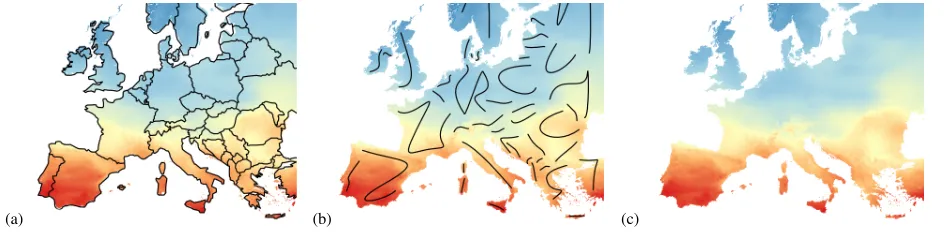
Many phenomena are collected and aggregated based on administra-tive subdivisions that are current at the time of collection. When the data are strongly correlated to these subdivisions or when only a local investigation of the data is required, the inclusion of boundaries helps to emphasize the locality of the portrayed information. Geographical phenomena, however, are often not tied to constructed political sub-divisions and require a broader scope for analysis of the phenomena. This is most notably the case for continuous data such as statistical surfaces or data from the realm of geosciences such as climate data.

Fig. 16. Example for river line symbols being used as main locational aid. Source: Grosser Atlas zur Weltgeschichte, 1991.

Placing boundaries on top of these kinds of cross-boundary phenom-ena has long been recognized as unhelpful in many cases:

In the smallest scales, one often just uses a strongly gener-alised hydrographic network along with the coastlines [as a base map]. – E. Imhof, 1972

The addition of rivers to the map allows for a sense of location even when boundaries are not present. As shown in Fig. 16, sparse base maps with just a strongly generalised line network can be very effec-tive for comparison purposes. The rivers presented fulfill the task nor-mally covered by the boundaries in a map, giving a sense of location that is static across different maps and helps to locate items within the map. The importance of such additional features is most clearly pre-sented by Fig. 17(c). Though the lack of any boundaries ensures that the continuity of the phenomena is emphasized, locating countries on the inside of the subdivision (e.g., Hungary) is hard.

While the introduction of river networks is helpful to give a sense of location on a map, in some cases this information may not be avail-able or desired. Using boundary information instead, however, intro-duces several problems (see Fig. 17(a)). Closing off areas reintro-duces the perceived continuity of the phenomena as polygons inherently give a stronger sense of positioning of the data. This effect is even further amplified as colors are visually interpreted as more uniform within each polygon. Stenomaps introduce a new, less intrusive way to give a reference to location (see Fig. 17(b)) without implying dis-crete changes at boundaries. By removing the need to close off areas, the continuity of the described phenomena is better maintained. The inexactness of glyphs ensures that no exact location can be matched with the data. Nevertheless, similar to river networks, glyphs instill a sense of location allowing for comparisons between maps.

(a) (b) (c)

7 DISCUSSION ANDFUTUREWORK

Evaluation. The use of linear features to represent polygons is an

intriguing new concept that gives rise to stenomaps. We presented an algorithm for the automated construction of stenomaps and discussed a variety of use cases. The results are convincing and visually pleasing. It is, however, unclear how effective stenomaps are. To gauge the us-ability of stenomaps user studies should be performed in future work. A first step could be to test the recognizability. It should be tested if the proposed glyphs maintain sufficient information for users familiar with the input. After recognizability, task appropriateness should be tested for the different use cases. This will be harder to measure as the glyphs are dissimilar from existing techniques, thereby risking a bias towards more familiar methods. However, task-based evaluation, such as estimation of hurricane damage probabilities over space could provide a useful means of comparison with conventional techniques. Testing the usability of this new method would give a better insight in the strengths and weaknesses of the method; possibly spurring further development.

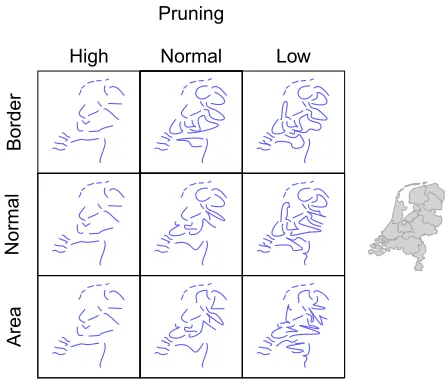
Methodology.The generation of glyphs can be steered using two

dif-ferent parameters. First, by changing the level of pruning of the medial axis the complexity of the final glyph can be determined. Second, the computed backbone can be set to better represent area or boundary. The interplay of these variables allows for a large range of design op-tions (see Fig. 18). These opop-tions allow map designers more choice over the shape of the glyphs. However, the question arises if it is possible to define a base setting appropriate for most maps. This is already partially the case as differently shaped polygons within one map are presented using the same settings. Preliminary experiments, however, show that a standard base setting across different maps is un-likely as different maps require different levels of detail. Subdivisions with uniquely shaped polygons require less exact detail than more uni-formly shaped subdivisions (e.g., the difference between the states of the USA and the countries of Europe).

The medial axis as a shape-descriptor is very suitable for the cre-ation of glyphs. It allows both feature points to be detected and an efficient computation of the available space. The medial axis is a rep-resentation of the polygon space, however it is not necessarily a fair sample. In parts where the inscribed circles are large the medial axis may be far removed from sections of the polygon. Thus, the medial axis may be a false sample when computing the maximum minimum distance to the backbone (Section 4.3). Misrepresenting the area of the polygon can result in visual artifacts as sections of the polygon may not be taken into account. The boundary representation that is part of the scoring function counteracts these effects. Though misrep-resentation is unlikely, future work might investigate if other distance measures can give a better representation of the area.

Glyphs. Glyph representations allow a significant abstraction from

the original input. This level of abstraction is a main feature of the stenomap, but also brings forth new considerations. The representa-tion of polygons through glyphs is very useful when informarepresenta-tion about a subdivision is shown. The extreme level of abstraction, however, im-plies that glyphs maintain their meaningfulness only while in context. When less context is present a larger amount of detail should be main-tained in the glyphs. Displaying more detail within the glyph, how-ever, reduces the advantage of using glyphs. Another consideration introduced by the extreme abstraction of glyphs is their uniqueness. As glyphs are highly abstracted, similarly shaped polygons may end up with a near similar glyph. While glyphs are distinguishable through their positioning in the subdivision, having uniquely shaped glyphs may be beneficial in some maps where lookup tasks are important. Similar shapes create a visual connection, which might counteract the data being presented. For future work it would be interesting to see if unique glyphs can be guaranteed. Taking similarity into account during the creation of glyphs is likely undesirable when fast compu-tation is essential, since it introduces dependencies between subprob-lems and inhibits parallel computation.

The minimal information maintained in glyphs is still sufficient to give an inexact description of the input shape. It can be argued that

Low

High

Normal

Border

Normal

Area

Pruning

Fig. 18. A sample of the parameter space defined by the user parame-ters affecting complexity and polygon representation.

the main strength of glyphs is bound by their subconscious relation to the original input shapes. There is a danger that when the user has no knowledge about those shapes, glyphs could lose part of their strength. We would argue, however, that the glyph in itself becomes a representation of the shape that is sufficient for many tasks where precise geometry of polygonal regions is not central. Glyphs supply sufficient information even when the input division may not be well known (e.g., Fig.14).

Through their simplicity glyphs make an interesting case for user interaction. Clearly, glyphs can be used as an additional visualization tool. Glyphs reduce the visual input complexity, which can be bene-ficial when a high-level overview is required. Their smoothness and simplicity, however, also makes glyphs intriguingly suitable for swipe interaction. Through swipe gestures item selection or map interaction could be achieved. For this use case, unique glyphs would be required. Stenomaps are very efficient when exact boundaries of a subdivi-sion are not needed but a general representation of the shape is helpful. They also offer several unique graphical variations that are applicable to various common use-cases. But by their intended nature of being a one-dimensional visual shorthand for a two-dimensional object they are still tied to size differences of the input polygons. Succinctly, they share the problems of polygons when directly trying to display quanti-ties by size modification. However, as they are one-dimensional, they conceptually offer the opportunity to address this fundamental limita-tion of cartography. Thus, future work might explore if it is feasible to ensure that all glyphs have equal length. As glyphs are independent of each other this could, for example, allow for distortion-free car-tograms. However, it is unclear whether such an approach would be feasible. First, different sized polygons might coexist in a map (e.g., Luxembourg and Russia). Using too small glyphs would be unsuit-able for large polygons, whereas too large glyphs could quickly fill up small polygons. Second, even given equal length, glyph shape still af-fects the visual saliency. Nevertheless, stenomaps might point the way towards a distortion-free solution of the value-by-area problem.

ACKNOWLEDGMENTS

REFERENCES

[1] D. Auber, C. Huet, A. Lambert, B. Renoust, A. Sallaberry, and A. Saulnier. Gospermap: Using a gosper curve for laying out hierar-chical data.IEEE Transactions on Visualization and Computer Graphics, 19(11):1820–1832, 2013.

[2] X. Bai and L. Latecki. Discrete skeleton evolution. InEnergy

Mini-mization Methods in Computer Vision and Pattern Recognition, pages

362–374. Springer, 2007.

[3] X. Bai, L. Latecki, and W.-Y. Liu. Skeleton pruning by contour partition-ing with discrete curve evolution.IEEE Transactions on Pattern Analysis

and Machine Intelligence, 29(3):449–462, 2007.

[4] M. de Berg, O. Cheong, M. van Kreveld, and M. Overmars.

Compu-tational geometry: algorithms and applications. Springer, 3rd edition,

2008.

[5] M. de Berg, M. van Kreveld, and S. Schirra. A new approach to subdivi-sion simplification. InProceedings of the 12th International Symposium

on Computer-Assisted Cartography, volume 4, pages 79–88, 1995.

[6] A. Beristain, M. Gra˜na, and A. Gonzalez. A pruning algorithm for stable voronoi skeletons. Journal of Mathematical Imaging and Vision, 42(2-3):225–237, 2012.

[7] J. Bertin. Graphische Semiologie. Diagramme, Netze, Karten. Gruyter, 1973.

[8] H. Blum. A transformation for extracting new descriptors of shape.

Mod-els for the perception of speech and visual form, 19(5):362–380, 1967.

[9] C. Brewer and B. Buttenfield. Mastering map scale: balancing workloads

using display and geometry change in multi-scale mapping.

Geoinfor-matica, 14:221–239, 2010.

[10] K. Buchin, W. Meulemans, and B. Speckmann. A new method for sub-division simplification with applications to urban-area generalization. In

Proceedings of the 19th ACM SIGSPATIAL GIS, pages 261–270, 2011.

[11] D. Burghardt, C. Duchˆene, and W. Mackaness, editors.Abstracting Geo-graphic Information in a Data Rich World - Methodologies and

Applica-tions of Map Generalisation. Springer, 2014.

[12] B. Buttenfield and R. McMaster, editors. Map Generalization - Making

Rules for Knowledge Representation. Longman, 1991.

[13] P. De Casteljau. Outillages m´ethodes calcul. Technical report, A. Citro¨en, 1959.

[14] D. Douglas and T. Peucker. Algorithms for the reduction of the number of points required to represent a digitized line or its caricature.

Carto-graphica, 10(2):112–122, 1973.

[15] R. Drysdale, G. Rote, and A. Sturm. Approximation of an open polygonal curve with a minimum number of circular arcs and biarcs.Computational

Geometry: Theory and Applications, 41(1-2):31–47, 2008.

[16] U. Freitag. Kartographische Konzeptionen - Cartographic

Concep-tions, chapter Die Eigenschaften der kartographiscehn

Darstellungsfor-men, pages 115–132. Freie Universitt Berlin, 1992.

[17] A. van Goethem, W. Meulemans, A. Reimer, H. Haverkort, and B.

Speck-mann. Topologically Safe Curved Schematization. The Cartographic

Journal, 50(3):276–285, 2013.

[18] G. Hake, D. Gr¨unreich, and L. Meng.Kartographie Visualisierung

raum-zeitlicher Informationen. Walter de Gruyter, Berlin, New York, 2002.

[19] M. Heimlich and M. Held. Biarc approximation, simplification and smoothing of polygonal curves by means of Voronoi-based tolerance

bands. International Journal of Computational Geometry and

Applica-tions, 18(3):221–250, 2008.

[20] H. Imai and M. Iri. Computational-geometric methods for polygonal ap-proximations of a curve.Computer Vision, Graphics and Image Process-ing, 36(1):31–41, 1986.

[21] E. Imhof.Thematische Kartographie. Walter de Gruyter, 1972.

[22] M. Kraak and F. Ormeling.Cartography: Visualization of Spatial Data,

Second Edition.Addison Wesley Longman, subsequent edition, 2003.

[23] W. Mackaness and A. Reimer. Generalisation in the context of schema-tised maps. InAbstracting Geographic Information in a Data Rich World.

Methodologies and Applications of Map Generalisation. Springer, 2014.

[24] W. A. Mackaness, A. Ruas, and L. T. Sarjakoski, editors.Generalisation of Geographic Information: Cartographic Modelling and Applications

(International Cartographic Association). Elsevier Science, 1st e edition,

April 2007.

[25] D. Macrini, S. Dickinson, D. Fleet, and K. Siddiqi. Object

categoriza-tion using bone graphs. Computer Vision and Image Understanding,

115(8):1187–1206, 2011.

[26] A. Masood and S. Ejaz. An efficient algorithm for robust curve fitting

using cubic Bezier curves. InAdvanced Intelligent Computing Theories

and Applications, LNCS 6216, pages 255–262, 2010.

[27] X. Mi, D. DeCarlo, and M. Stone. Abstraction of 2D shapes in terms

of parts. InProceedings of the 7th International Symposium on

Non-Photorealistic Animation and Rendering, pages 15–24, 2009.

[28] O. Neurath. Gesellschaft und Wirtschaft. Bildstatistisches Elementarw-erk. Bibliographisches Institut Leipzig, 1931.

[29] R. Ogniewicz and O. K¨ubler. Hierarchic voronoi skeletons. Pattern

recognition, 28(3):343–359, 1995.

[30] P. Picasso and S. Galassi.Picasso’s One-Liners. Artisan, 1997. [31] A. Reimer. Squaring the circle? bivariate colour maps and jacques bertins

concept of disassociation. InInternational Cartographic Conference, pages 3–8, 2011.

[32] P. Schneider. An algorithm for automatically fitting digitized curves. In

Graphic Gems, pages 612–626. Academic Press Professional, 1990.

[33] D. Shaked and A. Bruckstein. Pruning medial axes.Computer Vision and

Image Understanding, 69(2):156–169, 1998.

[34] W. Shen, X. Bai, R. Hu, H. Wang, and L. Latecki. Skeleton growing and pruning with bending potential ratio. Pattern Recognition, 44(2):196– 209, 2011.

[35] E. Spiess. Eigenschaften von kombinationen graphischer variablen.

Grundsatzfragen der Kartographie, pages 280–293, 1970.

[36] M. Stone and T. DeRose. A geometric characterization of parametric cubic curves.ACM Transactions on Graphics, 8(3):147–163, 1989. [37] S. Tak and A. Cockburn. Enhanced spatial stability with hilbert and

moore treemaps. IEEE Transactions on Visualization and Computer

Graphics, 19(1):141–148, 2013.

[38] N. Trinh and B. Kimia. Skeleton search: Category-specific object recog-nition and segmentation using a skeletal shape model.International

Jour-nal of Computer Vision, 94(2):215–240, 2011.

[39] M. Visvalingam and J. Whyatt. Line generalisation by repeated elimina-tion of points.Cartographic Journal, 30(1):46–51, 1993.

[40] M. Wattenberg. A note on space-filling visualizations and space-filling

curves. InIEEE Symposium on Information Visualization, pages 181–