White Rose Research Online URL for this paper:
http://eprints.whiterose.ac.uk/139567/
Version: Accepted Version
Article:
Baldivieso Monasterios, P. and Trodden, P. orcid.org/0000-0002-8787-7432 (2018) Model
predictive control of linear systems with preview information: feasibility, stability and
inherent robustness. IEEE Transactions on Automatic Control. ISSN 0018-9286
https://doi.org/10.1109/TAC.2018.2886156
© 2018 IEEE. Personal use of this material is permitted. Permission from IEEE must be
obtained for all other users, including reprinting/ republishing this material for advertising or
promotional purposes, creating new collective works for resale or redistribution to servers
or lists, or reuse of any copyrighted components of this work in other works. Reproduced
in accordance with the publisher's self-archiving policy.
[email protected]
https://eprints.whiterose.ac.uk/
Reuse
Items deposited in White Rose Research Online are protected by copyright, with all rights reserved unless
indicated otherwise. They may be downloaded and/or printed for private study, or other acts as permitted by
national copyright laws. The publisher or other rights holders may allow further reproduction and re-use of
the full text version. This is indicated by the licence information on the White Rose Research Online record
for the item.
Takedown
If you consider content in White Rose Research Online to be in breach of UK law, please notify us by
Model predictive control of linear systems with preview
information: feasibility, stability and inherent robustness
P. R. Baldivieso Monasterios and P. A. Trodden, Member, IEEE
Abstract—The use of available disturbance predictions within a nomi-nal model predictive control formulation is studied. The main challenge that arises is the loss of recursive feasibility and stability guarantees when a persistent disturbance is present in the model and on the system. We show how standard stabilizing terminal conditions may be modified to account for the use of disturbances in the prediction model. Robust stability and feasibility are established under the assumption that the disturbance change across sampling instances is limited.
Index Terms—Linear systems; Uncertain systems; Predictive control for linear systems; Constrained control
I. INTRODUCTION
The stability and robustness of model predictive controllers has been investigated extensively over the last few decades, and the theoretical foundations are now mature [1]. Ultimately, the purpose of any feedback controller is to reduce the effects of uncertainty on a plant, and accordingly the MPC literature is—by and large—separable into three, depending on whether or how uncertainty is considered: nominal MPC for deterministic (i.e.disturbance-free) systems, robust MPC for systems subject to bounded uncertainty and stochastic MPC for systems subject to uncertainties for which a probabilistic description is available [2]. While the fundamental conditions for stabilizing nominal controllers have been known for some time [3], progress has been more recent in robust and stochastic forms of MPC [1]. Even so, nominal MPC remains the most popular choice in practical applications, owing to its greater simplicity with respect to both design and computation. The drawback to nominal MPC is, of course, that the guarantees provided by the controller are indeed only nominal; instances of zero robustness when the MPC controller employs a nominal model but the real system is subject to an additive disturbance are well documented [4]. Consequently, the inherent robustness properties of nominal MPC have been investigated thoroughly, and necessary and sufficient conditions are well established [5], [6].
Despite these successes, a problem that has received relatively little attention is that of regulation of a disturbed system by nominal MPC when aforecastorpreview informationof future disturbances is available for use in the prediction model. This problem does not exactly fit the descriptions of robust or stochastic MPC for regulation, but is closely related to topic of tracking, wherein it has been known for some time that a disturbance model must be included in the predictions in order to obtain offset-free tracking [7]; in that context, different classes of disturbance signals have been investigated, including piecewise constant [7]–[9] and periodic [10]–[12].
Thispreview controlproblem [13] that we study is motivated by applications in,inter alia, power systems [14], wind energy [15]–[17], water networks [18] and automotive control [19]. Another motivation is, as we show in Section II, the optimal control problem that arises in
distributedMPC. The common feature is the availability of (possibly accurate) predictions about an exogenous disturbance acting on the plant, obtained from sensors or otherwise: for example, wind gusts
Work was supported by the Harry Nicholson PhD Scholarship, Department of Automatic Control & Systems Engineering, University of Sheffield.
P. R. Baldivieso Monasterios and P. A. Trodden are with the Department of Automatic Control & Systems Engineering, University of Sheffield, Sheffield, UK{p.baldivieso, p.trodden}@sheffield.ac.uk
acting on a turbine may be predicted by LiDAR, while the load disturbance in a power network is partly deterministic (scheduled by contract) and hence predictable. Most approaches to preview MPC focus on formulating a controller in the setting of the application, and then demonstrating the benefits to closed-loop performance of including accurate preview information; stability guarantees are largely lacking. An exception is the schemes based on robust MPC: [18] proposes a controller that uses knowledge of a deterministic demand in a tube-based robust MPC scheme. The approach of [14] uses preview information to bound uncertainties, and a parametrization of the control law in terms of the disturbance is used obtain a robust controller. The uncertain load scheduling problem tackled by [20] employs a robust controller acting on the uncertain error dynamics, thus eliminating the scheduled disturbance in the prediction model.
The aim of this note is to study the direct use of a disturbance prediction within a nominal MPC formulation for regulation, and develop conditions for the recursive feasility, stability and inherent ro-bustness of such a controller without using the well-known techniques from tracking or resorting to taking a robust or stochastic approach. We consider a linear time-invariant, constrained system subject to an additive disturbance, with the assumption that a sequence of future disturbances (over the horizon of the controller) is known to the controller at the current time, but—given the non-deterministic nature of the disturbance—this sequence may change arbitrarily (within a bounded set) at the next step, thus ispersistent. It is known that nominal MPC controllers for linear systemsdopossess robustness to bounded additive disturbances [6], but these results are restricted to the case where the prediction model omits the disturbance. Technical challenges arise when the disturbance is included in the prediction model, which mean that feasibility and stability are not assured, even when standard stabilizing terminal conditions are employed.
Our contributions are the following: we modify standard terminal ingredients for nominal MPC [21] to account for the disturbance appearing in the prediction model; we consider a general form of terminal conditions permitting the use of a nonlinear terminal control law. Under the modifications, the ill-posedness of the optimal control problem is removed, and the desirable properties of invariance of the terminal set and monotonic descent of the terminal cost hold for the perturbed model. Then we study the inherent robustness (to changing preview information) of the controlled system; we find that, as in inherently robust nominal MPC, the system states converge to a robust positively invariant set around the origin, the size of which depends on the limit assumed (or imposed) on the step-to-step change of the disturbance predictions. Illustrative examples show the advantage of including the disturbance in the prediction model: the region of attraction is larger than that for same controller omitting the disturbance information.
and conclusions are made in Section VI.
Notation and basic definitions:R+is the set of non-negative reals
andNis the set of positive integers. The set of symmetric positive
semidefinite n×nmatrices is Sn+ and the set of positive definite ones is Sn++. We use normal face to denote a real-valued vector,
and boldface to denote a sequence of vectors.|x|denotes a generic norm of a vectorx∈Rn;kxk2
Qdenotes the quadratic formx⊤Qx inx∈Rn, whereQ∈Rn×n. For setsA ⊂RnandB ⊂Rn, the Minkowski sum isA ⊕ B,{a+b:a∈ A, b∈ B}. The notation
A−1(X)
represents the preimage of the setX under the matrixA,
i.e. A−1
(X),{x:Ax∈X}. A setX⊆Rnis positively invariant for a (autonomous) system x+ = f(x)
, where f:Rn 7→ Rn, if
x∈X implies f(x) ∈X. A set X ⊆Rnis control invariant for a (non-autonomous) system x+ =f(x, u)
and input setU, where
f:Rn×Rm7→Rn, if for allx∈X there exists au∈Usuch that
f(x, u)∈X. A C-set is a closed and bounded (compact) convex set containing the origin; if the origin is in the interior, then it is a PC-set. An LTI systemx+=Ax+Bu
is reachable (controllable from the origin) if, for anyx1∈Rn, there exists a sequence of controls that
steers the state fromx(0) = 0tox1 in finite time. When it is clear
from the context, and in order to keep notation simple, we reserve
k as the sampling instant andias the prediction step; that is,x(k)
denotes a state at sampling instant k, whilex(i) denotes ani-step ahead prediction of x; where confusion may arise, we writex(k+i)
to denote the latter.
II. PROBLEM SETUP AND BASIC FORMULATION
A. System description and control objective
Consider the regulation problem for a discrete-time, linear time-invariant (LTI) system subject to an additive disturbance:
x+
=Ax+Bu+w (1)
wherex∈Rn,u∈Rm, w∈Rn are, respectively, the state, input, and disturbance at the current time, and x+
is the successor state. The control objective is to regulate the state to the origin, despite the action of the disturbance, while satisfying any constraints on states and inputs:
x∈X⊂Rn, u∈U⊂Rm
Assumption 1 (Basic system assumptions). The pair (A, B) is reachable, and the matrices (A, B)are known.
Assumption 2(Constraint sets). The setsXandUare PC-sets; the
setWis a C-set.
We make the following assumption about the preview information available to the controller at the time it makes control decisions:
Assumption 3(Information available to the controller).
1) The statex(k)and disturbancew(k)are known exactly at time k; the future disturbances are not known exactly but satisfy w(k+i)∈W, i∈N.
2) At any time stepk, apredictionof future disturbances, over a finite horizon, is available.
Full state availability is a standard assumption, but disturbance measurement availability is not; this might be restrictive but can arise in problems in, for example, power systems and, as we show in Section II-C, distributed MPC.
The main focus of the note is on the second part of Assumption 3: the availability of disturbance predictions. Our aim is to study how such information can be used within a nominal MPC formulation, and establish conditions for feasibility, stability and inherent robustness of the resulting controller and closed-loop system. Note that we do not
assume anything about theaccuracyof the disturbance predictions, and in fact will permit the predictions to vary over time (in which case it is implicit that earlier predictions were not accurate).
B. A basic MPC formulation with disturbance information
We study an MPC formulation that would arise from the direct (and perhaps naïve) inclusion of disturbance predictions in a nom-inal MPC problem for regulation, without using techniques from tracking MPC to handle it. As per the preceding assumptions, the controller has knowledge of the current statexand disturbancew
but, additionally, apredictionof the future disturbances. We define the disturbance prediction at the current time to be a sequence
w,w(0), w(1), . . . , w(N−1) , wherew(0) =w(the measured disturbance), with that and each future value of the sequence lying within the bounded setW. The optimal control problem for(x,w)is
P(x;w) : min
VN(x,u;w) :u∈ UN(x;w)
whereUN(x;w)is defined by, fori= 0. . . N−1,
x(0) =x,
x(i+ 1) =Ax(i) +Bu(i) +w(i), x(i)∈X,
u(i)∈U, x(N)∈Xf.
In this problem, the cost function comprises, in the usual way, a stage cost plus terminal penalty:
VN(x,u;w),Vf x(N);w+ N−1
X
i=0
ℓ x(i), u(i);w,
whereℓ:Rn×Rm7→R+,Vf:Rn7→R+; both depend, in a way
that is to be defined, on the disturbance sequence. The domain of this problem isXN(w) , x∈X:UN(x;w)6=∅ , and depends onw. The objective of the controller is to steer the system towards its
equilibrium despite the disturbances; when the disturbance ispersistent
then regulation is merely to a neighbourhood of the origin. In this case, we aim to achieve regulation to a neighbourhood of the origin using only nominal MPC,i.e. avoiding a robust formulations.
The solution of this problem at a state xand with disturbance sequencewyields an optimal control sequence
u0(x;w), u0
(0;x,w), u0(1;x,w), . . . , u0(N−1;x,w) .
The application of the first control in the sequence defines the control law u = κN(x;w) = u0(0;x,w). At the successor state x+ =
Ax+BκN(x;w) +w(0;w), the problem is solved again, yielding a new control sequence. Motivated by the limited accuracy of any disturbance prediction, the disturbance sequence used in the problem atx+
may change arbitrarily tow+, and is not necessarily equal to the tail of the previous sequencew.
C. A motivating application: distributed MPC
Our problem description can arise naturally in distributed forms of MPC. Consider the two dynamically coupled subsystems
x+1 =A11x1+B1u1+A12x2
x+
2 =A22x2+B2u2+A21x1
and suppose each subsystem controller p∈ {1,2} has an optimal control problem of the form
whereUp,N(xp;wp)is defined by
xp(0) =xp,
xp(i+ 1) =Appxp(i) +Bpup(i) +wp(i),
xp(i)∈Xp,
up(i)∈Up,
xp(N)∈Xp,f.
Suppose that, at some sampling instant, controller1solves its problem first (assuming some information about w1—in the simplest case
w1=0) to obtain an optimized future control sequenceu01(x1)and
associated sequence of state predictions, x01(x1). If the controller
then shares these predictions with controller 2, then controller 2
receives preview information w2 =x01(x1) available to use in its
own problem. In fact, w2 fits exactly with Assumption 3, for the
first element w2(0) =x1 is known accurately, while the remaining
elements are subject to change at the next sampling instant (after controller1solves its optimization problem once more).
Distributed MPC schemes essentially differ in how they use this information: it is known that the direct inclusion into the MPC formulation, as we have illustrated here, is problematic, and therefore iterative [22] and robust [23], [24] methods are typically used.
D. Stabilizing conditions for nominal MPC and issues that arise from including preview information
When the prediction model omits the disturbance, an established approach to ensuring desirable properties of the controller and closed-loop system is to design the cost and terminal set to satisfy some standard conditions [21]. In particular, when the model employed is
x+
=Ax+Buand neither the terminal set nor the cost function depend onw, the latter are constructed to satisfy the following:
Assumption 4(Terminal set properties). The setXf ⊂Xis a PC-set.
Assumption 5 (Cost function bounds). The functions ℓ(·,·), Vf(·)
are continuous, withℓ(0,0) = 0,Vf(0) = 0and such that, for some
c1>0,c2>0,a >0,
ℓ(x, u)≥c1|x|afor allx∈ XN, u∈U
Vf(x)≥c2|x|afor allx∈Xf
Assumption 6(Basic stability assumption). For allx∈Xf,
min
u∈U
Vf(Ax+Bu) +ℓ(x, u) :Ax+Bu∈Xf ≤Vf(x).
Assumption 7 (Control invariance of Xf). The setXf is control invariant forx+
=Ax+Buand the setU.
In turn, each of thecontrollability setsX0,X1, . . . ,XN, where
Xi+1={x∈X:∃u∈Usuch thatAx+Bu∈ Xi}, withX0=Xf, is control invariant forx+=Ax+BuandU, and these sets arenested:XN⊇ XN−1⊇ · · · ⊇ X1⊇ X0. Furthermore,
the setXN (and XN−1) is positively invariant forx+ =Ax+Bu
under the MPC control lawu=κN(x)and admissible with respect to the constraints. Consequently, ifx(0)∈ XN then (i) the optimal control problem is recursively feasible, (ii) constraints are satisfied for all times, and the origin is asymptotically stable for the closed-loop system, with region of attractionXN [21].
When disturbances are present in the model, the same ingredients fail to attain the same guarantees, and several issues arise.
• Ill-posed objective. For the perturbed dynamics,(x= 0, u= 0)
is not, in general, an equilibrium pair for the system. Conse-quently, employing a cost function that satisfies Assumptions 5
and 6 will not ensure that the value function satisfies the conditions of a Lyapunov function.
• Loss of invariance ofXf. Control invariance ofXf forx+ =
Ax+Budoes not imply control invariance forx+
=Ax+Bu+ w, even when wis constant. Invariance of Xf is anecessary
condition for the controllability sets to be control invariant and nested when state constraintsXare present [25].
• Loss of nesting of the controllability sets. The controllability sets
are defined by the iteration
Xi+1=X∩A− 1
Xi⊕ −BU⊕ −{w(N−i)}, (2)
with X0 =Xf. The final summand in (2) is problematic, for
{w(N−i)} is a point, not a set containing the origin, and therefore inducestranslationof the controllability sets between iterations. Moreover, ifAis unstable, then with each iteration the controllability set is shifted further away as disturbance propagates through the unstable predictions. The implication is thatXN is not control invariant forx+=Ax+Bu+w, and recursive feasibility may not be easy to establish, even ifXf is control invariant for the terminal dynamics.
III. MODIFICATIONS TO THE COST AND TERMINAL INGREDIENTS
In this section, we develop modifications to the cost ℓ(·,·) and terminal ingredients Vf(·), Xf for the model predictive controller that aim to overcome the first two of the fundamental issues outlined in the previous section. With respect to the third issue, we show in Section IV that recursive feasibility of the control problem can be established without relying on nestedness of the controllability sets; in fact, we show that a different kind of nested property holds here. Our approach is to modify the cost and terminal set using the available preview information. We assume a constant-disturbance terminal prediction model, take stabilizing ingredients designed for its nominal counterpart, and translate the costs and terminal set to account for the non-zero equilibrium caused by the disturbance; as we shall show, the resulting ingredients achieve the required properties of invariance and monotonicity with respect this new predicted equilibrium instead of the origin. The results in this section are essentially derived from known results on stabilizing MPC [21], but lay the foundations for our main results in Section IV.
A. Constant-disturbance terminal dynamics
In order to synthesize appropriate terminal ingredients, one first needs to consider the terminal (beyond the horizon) dynamics of the prediction model. This motivates the next assumption, regarding the disturbance sequence: by definition, the disturbance predictions are known only up toN steps ahead in the future, and therefore to consider the terminal dynamics we setup the predicted disturbance sequence in the following way:
Assumption 8. An admissibledisturbance sequencew ={w(0), . . . , w(N−1)}hasw(i)∈W,i= 0. . .(N−2), andw(N−1)∈
Wf ⊆W; we writew∈ W,W× · · · ×W×Wf. To account for
i≥N, the sequence is continued indefinitely by concatenation with wf ,w(i)
i≥N, withw(i) =wf(w),w(N−1)fori≥N. That is, the predicted disturbance is, afterN steps, constant and equal towf(w) =w(N−1), the final value in theN-length sequence
w. This final value lies in a subsetWf ⊆W; thus,wf:W 7→Wf. A constant terminal disturbance assumption is not necessarily restrictive; for example, [11] considers disturbance models that are integrating and reach a constant value.
byx =Ax+Bu+wf(w), withwf(w)constant for all prediction steps i≥N. At the next time instant, however,wf(w+) need not be equal towf(w), and we address this issue in Section IV. Until then, for simplicity of notation we refer towf(w)aswf.
B. Equilibria of the terminal dynamics
To proceed, we first assume the availability of terminal ingredients for the nominal system; in the sequel, the overbar notation denotes a function or set pertaining to the nominal dynamicsx+=Ax+Bu
.
Assumption 9. There is known a setX¯f and functions¯ℓ(·,·),V¯f(·)
satisfying Assumptions 4–7 for the dynamics x+
=Ax+Buand constraint sets(βxX, βuU), whereβx, βu∈[0,1).
The setX¯f is a control invariant set (for the nominal dynamics) that resides withinβxX, which is the state constraint set scaled to allow for the effect of non-zero disturbances on the terminal dynamics; the selection of suitable scaling factors βx andβu is described in the sequel. Assumption 9 implies the existence of a (possibly set-valued) control law, uf:Rn7→2
Rm
that induces invariance of the setX¯f
with respect to the nominal dynamics:
uf(x) =
u∈βuU:Ax+Bu∈X¯f,
¯
Vf(Ax+Bu) + ¯ℓ(x, u)≤V¯f(x) , forx∈X¯f. (3)
We denote the system x+
= Ax+Bu under the control law
u= ¯κf(x)—where, if necessary,¯κf(x)is an appropriate selection fromuf(x), but is otherwise equal touf(x)—asx+ =f¯κf(x) =
Ax+B¯κf(x) (so thatfκ¯f: ¯Xf 7→ X¯f). The following result is
an immediate consequence of the existence ofκ¯f(·) satisfying the conditions of Assumption 4–7.
Lemma 1(Stabilizing terminal control law). Suppose Assumptions 1 and 9 hold. The origin is an asymptotically stable equilibrium for the systemx+=f
¯
κf(x), with region of attractionX¯f.
The difficulty with translating the terminal ingredients to the new steady state or equilibrium point of the system perturbed bywf is that this point is not immediately known, since the terminal control law is nonlinear and/or set-valued. The approach we take is to linearize the terminal dynamics and control law around the equilibrium point
x= 0∈X¯f, for which we make the following assumption.
Assumption 10. κ¯f(·)is continuous overX¯f, with¯κf(0) = 0, and
continuously differentiable in a neighbourhood ofx= 0.
In reality, this is a mild assumption: a ready choice of¯κf(·)is a linear, stabilizingK. Even if ¯κf(·) is piecewise linear in order to maximize the size of X¯f (as in [26]), the control law is typically linear (for a linear system) in a neighbourhood of the origin whenX
and Uare PC-sets. Then the linearization ofx+=f ¯
κf(x)yields
Π, ∂κ¯f(x)
∂x
x=0
; Φ, ∂ Ax+Bκ¯f(x)
∂x
x=0
=A+BΠ (4)
from which the equilibrium point of the linearized system x+
= Φx+wf is
xf(wf) = Ψwf, uf(wf) = ΠΨwf
whereΨ, I−Φ−1
. In view of Lemma 1 and Assumption 10,Φ = (A+BΠ)is well defined and strictly stable, henceΨ = (I−Φ)−1
exists and is unique. This proves the following.
Lemma 2 (Existence of equilibrium). Suppose Assumptions 1, 9 and 10 hold. The pointxf(wf) exists and is the unique equilibrium of
x+
= Φx+wf, withwf constant.
C. Modified terminal conditions: translation and properties
We propose to translate the cost function, terminal sets and control law to this new point(xf, uf):
ℓ(x, u;wf),ℓ x¯ −xf(wf), u−uf(wf)
Vf(x;wf),V¯f x−xf(wf)
Xf(wf),X¯f⊕xf(wf)
κf(x;wf),κ¯f x−xf(wf)
+uf(wf)
The translated sets and functions are then the ones employed in the optimal control problem with perturbed prediction model. The main result of this section then establishes that the resulting terminal ingredients satisfy the required conditions (counterparts to Assumptions 4–6) for x+
=Ax+Bu+wf. First, the following assumption is required.
Assumption 11. There exist scalarsαx, αu∈[0,1)such that
ΨWf ⊆αxX ΠΨWf ⊆αuU
This assumption essentially limits the size of the terminal distur-bance set, Wf, with respect to the state and input constraint sets.
Then the following result restores the stability properties.
Proposition 1. Suppose that Assumptions 1–3, 8–11 hold. For any fixedwf ∈Wf, (i) the set
Xf(wf) = ¯Xf⊕xf(wf) (5)
is positively invariant forx+
=Ax+Bκf(x;wf) +wf, and (ii) the
functionsℓ(x, u;wf)andVf(x;wf)satisfy
Vf [Ax+Bκf(x;wf) +wf];wf
+ℓ x, κf(x;wf);wf
≤Vf(x;wf)for allx∈Xf(wf).
Furthermore, (iii)Xf(wf)⊆X, andκf(Xf;wf)⊆Uifαx+βx≤1
andαu+βu≤1. Finally, (iv) the pointxf(wf)is an asymptotically
stable equilibrium point for the systemx+
=Ax+Bκf(x;wf) +wf.
The region of attraction isXf(wf).
This result implies that the set Xf(wf) is control invariant for the systemx+
=Ax+Bu+wf,wf constant, and input setU. In particular, the set is positively invariant forx+=Ax+Bκ
f(x;wf)+
wf. Within this set,Vf(·)is a control Lyapunov function. Thus, we have established stability of the predicted terminal dynamics to an equilibrium point under the assumption of a constant disturbancewf. In the next section, we consider the receding-horizon implementation of the optimal control problem, allowing the terminal disturbance to change across sample times but, at each sampling instant, remain constant beyond the end of the horizon.
Remark 1(Offset-free regulation and links with tracking and robust MPC). In view of the regulation objective, the stabilization of the perturbed system under constant disturbances toxf(wf) = Ψwf may
seem unambitious. Ultimately, however, this is an issue of available degrees of freedom: if x = 0 is required to be an equilibrium of x+
=Ax+Bu+wf, then standard results from offset-free tracking
inform us this is possible, in general, if and only ifm≥n—a strong condition that is typically not met unless the system is over-actuated. A pragmatic solution, then, can be to define some outputsy=Cx∈Rp,
withp≤m, and steer the states to values that satisfyyf =Cxf = 0
(or minimize ||Cxf||2). With the regulation goal in mind, such a
scheme requires careful (and application-dependent) design ofCin order to ensure that some states do not converge to values far from the origin.
the origin that the states of a perturbed systemx+
= Φx+w, under bounded w ∈W, can stay within is the minimal robust positively invariant (mRPI) set, given by the Minkowski summation
R∞, ∞
M
i=0
ΦiW.
There is a strong connection between this set and the equilibrium point xf(wf) = Ψwf under a constant disturbancewf:xf(wf)∈ R∞ and, similar to this summation,
xf(wf) = (I−Φ)−
1
wf = (I+ Φ + Φ
2
+. . .)wf =
∞
M
i=0
Φi{wf}.
IV. FEASIBILITY,STABILITY AND INHERENT ROBUSTNESS UNDER CHANGING DISTURBANCES
In this section, we analyse the properties of the MPC controller with the proposed cost and terminal set modifications, considering the possibility that the disturbance sequence provided to the controller changes over time. Given a disturbance sequencew, the set of states for which the problem P(x;w)is feasible is XN(w) = {x∈X: UN(x;w)6=∅}. The challenge that arises is a consequence of the receding horizon implementation of MPC: ifP(x;w)is feasible and
yields a solutionu0(x;w),{u0(0;x,w), u0(1;x,w), . . . , u0(N− 1;x,w)}, then the first control in this sequence is applied (the implicit
control law isκN(x;w),u0(0;x,w)), the system evolves tox+=
Ax+BκN(x;w)+w, and the problem to be solved at the subsequent time isP(x+
;w+). The question is, when is this problem feasible, given that the disturbance sequence may have changed (perhaps arbitrarily) fromw tow+?
A. Unchanging disturbance sequences
Our first results on feasibility and stability consider the artificial situation where the disturbance sequence is shifted in time but otherwise unchanged,i.e.the sequencew+is thetailof the sequence w, and the disturbance acting on the plant is equal to the first
element in the sequence at each sampling instant. These results, though immediate consequences of the preceding developments and standard results in MPC, form the basis for the more realistic case of a persistently changing disturbance sequence considered in Sec. IV-B. In order to present the results, we need to define some notation. For a disturbance sequencew=
w(0), w(1), . . . , w(N−2), w(N−1) , the associated tail is w˜(w) ,
w(1), . . . , w(N−1), w(N−1)
where the firstN−1elements ofware augmented by continuing the final value w(N−1) for one further step. The infinite-length disturbance sequencewN(k)is formed from concatenatingw(k)and
wf(k) where
wN(k) =
w 0;w(k)
, . . . , w N−1;w(k)
,wf(k) .
The latter is the infinite sequence of constant disturbances obtained by holding the final value ofw(k)—that is,wf(k) =
wf w(k) wherewf w(k)
=w N−1;w(k). Finally,wi(k), fori= 0. . . N,
is a version ofwN(k)of omitting the firstN−i.
The next result, and those in the remainder of the paper, suppose that Assumptions 1–3, 9–11 hold.
Proposition 2 (Feasibility under unchanging disturbance). Letw= {w(0), w(1), . . . , w(N−1)} ∈ W. Ifw+ = ˜w(w)
, then (i)x∈ XN(w)impliesx+=Ax+BκN(x;w) +w(0;w)∈ XN(w+). (ii)
Givenw(0), the set
∞
[
k=0
XN w(k)withw(k+ 1) = ˜w w(k)
is control invariant forx(k+ 1) =Ax(k) +Bu(k) +w(k)andU, wherew(k) =w 0;w(k)
. (iii) The unions of controllability sets are nested:
∞
[
k=0
XN wN(k)⊇
∞
[
k=0
XN−1 wN−1(k)
⊇ · · · ⊇
∞
[
k=0
X0 w0(k)
,
where
Xi+1(wi+1) =X∩A
−1
Xi(wi)⊕ −BU⊕ −{w(N−i)},
withX0(w
0) =Xf(wf), andwi(k+ 1) = ˜w wi(k).
Remark 2. Whereas the individual setsXN,XN−1, . . . ,X0are not
necessarily control invariant and nested, their unions are, provided the disturbance sequence updates by taking the tail.
Remark 3. Owing to the nilpotency of the dynamics of the disturbance sequence (that is,wN(k+ 1) = ˜w w(k)
converges fromw(0)to wf inN steps), the set unions in Proposition 2 are finitely determined:
∞
[
k=0
XN w(k)= N
[
k=0
XN w(k).
Recursive feasibility leads to the following result.
Proposition 3 (Exponential stability of xf(wf)). Let w(0) ∈ W
andx(0)∈ XN(w(0)). If the disturbance sequence is updated as
w(k+ 1) = ˜w w(k)
, and the disturbance applied to the system isw(k) =w 0;w(k), then the point xf(wf)is an exponentially
stable equilibrium for the systemx+
=Ax+BκN(x;w) +w. The
region of attraction isXN(w(0)).
Proposition 3 highlights the advantage of including the disturbance sequence in the prediction model and adjusting the terminal conditions accordingly: stability of a point is achieved. On the other hand, when the disturbance sequence isnotincluded in the prediction model, we have the following well-known result from the inherent robustness of nominal MPC [6], [21], specialized to this setting.
Lemma 3(Robust stability of nominal MPC). Letw(0)∈ W and x(0)∈Ωβ(w=0),x:VN0(x;w=0)≤β ⊂ XN(w=0). If
Wis sufficiently small, thenΩβ(0)is a robust positively invariant set
forx+
=Ax+BκN(x;0)+w. Moreover, the system states converge,
in finite time, to a robust positively invariant setΩα(0) ⊆Ωβ(0),
the size of which depends onW.
We do not attempt to qualify what is sufficiently small here; details can be found in,e.g., [21, Chapter 3]. The main point is that the states of the closed-loop system can be guaranteed to converge to a neighbourhood of the origin, rather than an equilibrium point, when the disturbance is omitted from the predictions.
B. Persistently changing disturbance predictions
We next consider the case where the disturbance sequence is permitted to change over sampling instances, but where the rate of change is limited. As a prerequisite to our developments, we consider the composite statez,(x,w)and define
ZN ,
z= (x,w) :w∈ W, x∈ XN(w) ⊂Rn+nN.
In view of the properties ofXNandW, this is a PC-set. The following lemma is a well established consequence of linearity of the system, continuity of the cost, and compactness of the constraint sets [6].
Lemma 4(K-continuity of the value function). The value function V0
N(·)satisfies
V0
N(z1)−VN0(z2)
≤σV(|z1−z2|)overZN, with
We exploit this continuity in bounding the rate of change of disturbance sequences, as follows, and ultimately in establishing robust stability.
Assumption 12. The disturbance sequence evolves asw+= ˜w(w)+ ∆w, where∆w =w+−w˜(w)∈∆W ⊆ W. Moreover,∆W is chosen such that
λ,max
|w−w′|:w∈ W,w′∈ W,(w−w′)∈∆W
satisfies
λ≤σ−1
V (ρ−γ)α
forρ∈(γ,1), whereγ= (1−c1/c3)∈(0,1)andc3≥c2≥c1>0,
andα >0such thatΩz
α,{z= (x,w) :VN0(z)≤α} ⊂ ZN. This assumption aims to bound the persistent change in the disturbance predictions across sampling times, in order that the unanticipated change is not so large that the stability of the controller is lost. The constantsc1 andc2 in this assumption are the same ones
from Assumption 5, which bound the stage and terminal costs. The constantc3 is from the upper bound on the MPC cost, derived in the
proof of Proposition 3; γ is the rate of the value function descent,
V0
N(x
+
,w˜(w))≤γVN0(x;w), in this result.
We then have the following, main result.
Theorem 1. Suppose Assumptions 1–3, 9–12 hold, and letz(0) = x(0),w(0)
∈ Ωz
β = {(x,w) : VN0(z) ≤ β} ⊂ ZN, for some
β≥α. The setΩzβ is positively invariant for the composite system
x+
=Ax+BκN(x;w) +w,
w+∈w˜(w)⊕∆W and the states of the system enterΩz
αin finite time and remain therein.
Corollary 1. If x(0) ∈ Ωβ w(0) = {x : x,w(0) ∈ Ωzβ} ⊂
XN w(0)), then the system statex(k)remains withinΩβ w(k)
= {x: x,w(k)
∈Ωz
β} ⊂ XN w(k)provided that the disturbance
sequence update rate is limited as specified. Morever, all optimization problems remain feasible, and for allk after some finite timek′
, the state enters and remains in a setΩα w(k′)={x: x,w(k′)∈
Ωz
α}whereα≤β.
Corollary 2. The region of attraction for the controlled system is
∞
[
k=0
Ωβ w(k)withw(k+ 1)∈w w˜ (k)⊕∆W.
Givenw(0), the setΩβ w(0) can be chosen to be the largest sublevel set of the value function within XN w(0); our result says then that the system converges to the smallest sublevel set that satisfies Assumption 12. Comparing this result with the result of Lemma 3, the potential advantage of the disturbance sequence inclusion becomes clear: the regions of attraction with and without the disturbance predictions are—using the same terminal sets in each optimal control problem—S
k=0Ωβ w(k)
andΩβ(0) respectively. Care must be taken, however, before conclusions are made, because a conventional nominal formulation (omitting the disturbance) permits the use of a larger terminal set (Xf ⊆Xcompared withX¯f ⊆βxX). The example in the next section shows that, despite this, the proposed scheme can lead to a larger robust region of attraction.
Remark 4 (Comparison with robust MPC). We have studied a nominal formulation including disturbance predictions and analysed its inherent robustness to persistently changing predictions. Theorem 1, based on Assumption 12, offers interesting theoretical insight but is not constructive and, thus, is of limited practical use: several constants and sublevel sets of the value function would need to be determined, which
has to be done numerically. Robust tracking MPC techniques, which could also be applied to this problem, offer an attractive alternative, with robust-by-design guarantees and a region of feasibility that is equal to the region of attraction and possible to characterize explicitly. However, robust techniques rely on constraint restrictions and robust invariant sets [1], neither of which a nominal formulation requires, which introduces a degree of complexity to the design.
V. ILLUSTRATIVE EXAMPLES
Consider the neutrally stable dynamics
x+
= "
1 1 0 1 #
x+ "
0.5 1
#
u+w (6)
with state and input constraints X = {x ∈ R2 :
kxk∞ ≤ 10},
U={u∈R:|u| ≤3}. The disturbance takes values in the C-set
W ={w = (w1, w2) ∈ R2:|w1| ≤ 2, w1 = w2}. The nominal
stage and terminal costs are quadratic:
¯
ℓ(x, u) =x⊤Qx+u⊤Ru V¯
f(x) =x⊤P x,
whereQ=I,R= 1, andP is solution of the Lyapunov equation
(A+BKf)⊤P(A+BKf)−P =−(Q+Kf⊤RKf)for a stabilizing gainKf ∈Rm×ncharacterizing the nominal terminal control law
¯
κf(x) =Kfx. The matricesΦandΠare determined according to (4), respectively, using the nominal terminal control law,Φ =AKf =
A+BKf andΨ = (I−AKf) −1
. The nominal terminal set,X¯f, and scaling constantsβx,βu, αx andαu are designed in line with the requirements of Assumptions 9 and 11:X¯f is the maximal constraint admissible invariant set for x+
=AKfxwithin the state setβxX
and input setβuU, whileΨWf andKfΨWf must fit withinαxX andαuUrespectively. With the assumption thatWf =W, we obtain
βx= 0.672,βu= 0.7,αx= 0.328andαu= 0.3.
We consider controlling the system from different initial states using a horizon ofN= 3 and the following disturbance predictions at each sampling instantk:
w(k) =
w0={+0.9,−0.9,−0.9} mod (k,5) = 0
w1={+0.9,+0.9,+0.9} mod (k,5) = 1
w2={−0.9,−0.9,−0.9} mod (k,5) = 2
w3={−0.9,+0.9,−0.9} mod (k,5) = 3 w4={0,0,0} mod (k,5) = 4
The disturbance prediction cycles persistently between five different sequences, while the disturbance applied to the plant at timek is always the first in the sequencew(k):i.e.w(k) =w 0;w(k)
, so that w(0) = +0.9, w(1) = +0.9, w(2) = −0.9, etc. Following Assumption 12, the value of the maximum disturbance variation is
λ= 3.17.
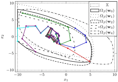
Figure 1 shows the trajectories of the closed-loop system from five different initial states, together with the level sets of the value function,
Ωβ(wi) ={x:VN0(x;wi)≤β}fori= 0. . .4andβ= 100. Each of the trajectories begins inΩβ(w0)—the level set corresponding to
the disturbance sequence atk= 0—and each subsequent state lies within the appropriateΩβ(w(k)); however,x(k)∈Ωβ(w(k))does not implyx(k+ 1)∈Ωβ(w(k)), as can be seen with the trajectory initialized atx(0) = [1.9 2.5]⊤, which begins inΩ
β(w0)and moves
outside toΩβ(w1). Since the disturbances and their predictions are
switching between non-decaying values, the states do not converge to zero, but rather to a neighbourhood of the origin.
Figure 2 compares the union ofβ= 100sublevel sets overw∈ W
−10 −5 0 5 10
−10
−5 0 5 10
x1
x2
X
Ωβ(w0)
Ωβ(w1)
Ωβ(w2)
Ωβ(w3)
[image:8.612.55.294.55.222.2]Ωβ(w4)
Fig. 1. Closed-loop trajectories of the system under switching disturbances, from different initial states, and the level setsΩβ(wi), i= 0. . .4, forβ=
100, corresponding to the disturbance sequenceswi, i= 0. . .4.
−10 −5 0 5 10
−10
−5
0 5 10
x1
i
x
2 i
X
S
wΩβ(w)
Ωstandard
[image:8.612.54.296.272.440.2]β
Fig. 2. The union of level setsΩβ(w)overw∈ Wforβ= 100, and the
corresponding level setΩstandard
β for a conventional MPC formulation.
large as Ωβ(w =0) in the proposed approach, because the latter requires the terminal set to fit withinβxX, rather than merelyXas the conventional controller requires. Despite this, theoverallregion of attraction for the proposed approach—as the union of Ωβ(w), following Corollary 1—is larger.
VI. CONCLUSIONS
We have studied the use of available disturbance predictions within a conventional nonlinear MPC formulation for regulation. Modifications to standard terminal conditions were presented. For unchanging disturbance predictions, recursive feasibility is guaranteed and exponential stability of the closed-loop system is established around an equilibrium point close to the origin. For arbitrarily changing disturbance sequences, stability of a robust positively invariant set is guaranteed, the size of which is related to the permitted step-to-step change of the disturbance sequence.
APPENDIX
A. Proof of Proposition 1
Consider some wf ∈ Wf. The pointxf =xf(wf) = Ψwf =
(I−Φ)−1
wf exists and is unique by Lemma 2. Let Xf(wf) =
¯
Xf ⊕ {xf}, and consider somex∈ Xf(wf) and a corresponding
z =x−xf ∈X¯f. The successor states are z+ =Az+B¯κf(z), which is inX¯f by construction, andx+
=Ax+Bκf(x;wf) +wf, which, using the control law definitionκ(x;wf) = ¯κf(x−xf)+Πxf, may be rewritten as
x+=Ax+Bκ¯f(x−xf) +BΠxf+wf
=A(z+xf) +B¯κf(z) +BΠxf+wf
=Az+Bκ¯f(z) + (A+BΠ)xf +wf
=z+
+ Φxf+wf
=z++xf
where the last line follows from Φxf +wf = ΦΨwf +wf =
(ΦΨ +I)wf, and sinceΨ = (I−Φ)−1 = (I−Φ)−1Φ +I, then
(ΦΨ +I) = Ψ and Ψwf = xf. Then x+ ∈ Xf(wf) because
z+
∈ X¯f. This establishes positive invariance of Xf(wf), for any
fixedwf ∈Wf, underu=κf(x;wf).
To prove constraint admissibility, by Assumption 11, we have that
ΨWf ⊆αxX andΠΨWf ⊆αuU, with αx, αu ∈ [0,1). On the other hand, by Assumption 9,X¯f ⊆βxXandκ¯f( ¯Xf)⊆βuU, with
βx, βu∈[0,1). ThenXf(Wf) = ¯Xf⊕ΨWf ⊆βxX⊕αxX⊆X, if αx+βx ≤ 1. Similarly, κf(Xf;Wf) = ¯κf( ¯Xf)⊕ΠΨWf ⊆
βuU⊕αuU⊆Uifαu+βu≤1.
Next, we prove the claimed properties of the functionsℓ(·,·)and
Vf(·). For somewf ∈Wf,x∈Xf(wf)and correspondingz=x−
xf ∈X¯f, we haveV¯f(z+)−V¯f(z)≤ −ℓ z,¯ κ¯f(z)by construction (Assumption 9). Then, forx+
=Ax+Bκf(x;wf) +wf,
Vf(x+)−Vf(x) = ¯Vf(x+−xf)−V¯f(x−xf)
= ¯Vf(z++xf−xf)−V¯f(z+xf−xf)
= ¯Vf(z
+
)−V¯f(z)
≤ −ℓ z,¯ κ¯f(z)
=−ℓ x¯ −xf,κ¯f(x−xf)
=−ℓ x¯ −xf, κf(x;wf)−Πxf
=−ℓ(x, u;wf)whereu=κf(x, wf) as required. Finally, the asymptotic stability of xf for the system
x+ =Ax+Bκ
f(x;wf) +wf follows from the bounds on Vf(·): for allx∈Xf(wf)
c1|x−xf|a≤Vf(x;wf)≤c2|x−xf|a
Vf(x+;wf)−Vf(x;wf)≤ −c1|x−xf|a. Thus,x→xf in the limit.
B. Proof of Proposition 2
For (i), given x ∈ XN(w) there exists a u(x;w) ∈
UN(x;w) with associated state predictions x(x;w) =
x0
(0;x,w), x0(1;x,w), . . . , x0(N;x,w) with x0(0;x,w) =x.
The successor state x+
= Ax +Bu0
(0;x,w) +w(0;w) = x0
(1;x,w), and so, by Proposition 1, the sequences
˜
x(x+;w) = x0
(1;x,w), . . . , x0(N;x,w), Ax0
(N;x,w) +Bκf x0(N;x,w);wf+wf
˜
u(x+;w) =u0(1;x,w), . . . , u0(N;x,w), κf x0(N;x,w);wf
˜
w(w) =w(1), w(2), . . . , w(N−2), w(N−1)
are feasible for all constraints that defineUN x+,w˜(w)
; in fact, the same solution omitting the terminal steps is also feasible for all constraints that defineUN−1 x+,w˜(w). Thus,x+∈ XN−1(w+)⊆
XN(w+) ifw+= ˜w(w).
Part (ii) follows directly from the above and recursion. If x ∈ XN(w)andx+∈ XN−1(w
+
u=κN(x;w), then, givenx(0)∈ XN w(0) and the disturbance update rule w(k+ 1) = ˜w w(k)
, the state trajectory x(k) k
remains within the union of XN w(k). Hence, the latter set is positively invariant for x+ =Ax+Bκ
N(x;w) +w, and control invariant forx+
=Ax+Bu+wandU.
The nested property of the set union follows from the key observation that, under the tail-updating law, wN(k + 1) = wN−1(k). Thus, since x(k) ∈ XN wN(k)
implies x(k + 1) ∈ XN−1 wN−1(k)
⊆ S
kXN−1 wN−1(k)
, it also implies
x(k + 1) ∈ XN wN(k + 1)
⊆ S
kXN wN(k)
. Therefore,
S
kXN wN(k)
⊇S
kXN−1 wN−1(k)
.
C. Proof of Proposition 3
From the definitions of Vf, ℓ and VN, and the bounds in Assumption 5, we have, for allx∈ XN(w)
V0
N(x;w)≥ℓ x, κf(x;wf);wf≥c1|x−xf|a,
while the fact that the costs are continuous and the setsXf,X,Uare PC-sets means there exists ac3≥c2>0such that
V0
N(x;w)≤Vf(x;wf)≤c2|x−xf|afor allx∈Xf(wf)
=⇒ V0
N(x;w)≤c3|x−xf|afor allx∈XN(w) Recursive feasibility and the descent property ofVf yields, for all
x∈XN(w),
V0
N(x
+
; ˜w)≤V0
N(x;w)−ℓ x, κf(x;wf);wf≤γVN0(x;w) where γ , (1−c1/c3) ∈ (0,1) (since c3 > c1 > 0). Thus,
V0
N x(k);w(k)
≤γkV0
N x(0);w(0)
, and, becausec1|x−xf|a≤
V0
N(x;w)≤c3|x−xf|a,
c1|x(k)−xf|a≤γkc3|x(0)−xf|a =⇒
|x(k)−xf| ≤cδk|x(0)−xf|
wherec,(c3/c1)1/a>0andδ,γ1/a∈(0,1).
D. Proof of Theorem 1
Consider somez = (x,w) ∈ ΩzN. We haveV0
N x
+
,w˜(w)≤ γV0
N(x,w)≤γβ. ByK-continuity,
V0
N(x
+
,w+)≤V0
N x
+
,w˜(w) +σV
w+−w˜(w)
.
Therefore, sinceσV w
+
−w˜(w)
≤σV(λ)≤(ρ−γ)α,
V0
N(x
+
,w+)≤γβ+ (ρ−γ)α≤ρβ < β.
Moreover, if x(0),w(0) ∈Ωz
β\Ωzα, then
VN0 x(1),w(1)
≤γVN0 x(0),w(0)
+ (ρ−γ)VN0 x(0),w(0)
≤ρV0
N x(0),w(0)
.
Consequently,V0
N x(k),w(k)
≤ρkβ, from which it follows that
V0
N x(k′),w(k′)
≤αafter some finitek′
.
REFERENCES
[1] D. Q. Mayne, “Model predictive control: Recent developments and future promise,”Automatica, vol. 50, pp. 2967–2986, 2014.
[2] B. Kouvaritakis and M. Cannon,Model Predictive Control: Classical, Robust and Stochastic. Springer, 2016.
[3] D. Q. Mayne, J. B. Rawlings, C. V. Rao, and P. O. M. Scokaert, “Con-strained model predictive control: Stability and optimality,”Automatica, vol. 36, pp. 789–814, 2000.
[4] G. Grimm, M. J. Messina, S. E. Tuna, and A. R. Teel, “Examples when nonlinear model predictive control is nonrobust,”Automatica, vol. 40, no. 10, pp. 1729–1738, 2004.
[5] ——, “Nominally robust model predictive control with state constraints,”
IEEE Transactions on Automatic Control, vol. 52, no. 10, 2007. [6] D. Limon, T. Alamo, D. M. Raimondo, D. Muñoz de la Peña, J. M.
Bravo, A. Ferramosca, and E. F. Camacho, “Input-to-state stability: A unifying framework for robust model predictive control,” inNonlinear Model Predictive Control: Towards New Challenging Applications, ser. Lecture Notes in Control and Information Sciences, L. Magni, D. M. Raimondo, and F. Allgöwer, Eds. Springer, 2009, vol. 384, pp. 1–26. [7] K. R. Muske and T. A. Badgwell, “Disturbance modeling for offset-free linear model predictive control,”J. Process Control, vol. 12, no. 5, pp. 617–632, 2002.
[8] L. Chisci and G. Zappa, “Dual mode predictive tracking of piecewise constant references for constrained linear systems,”International Journal of Control, vol. 1, pp. 61–72, Jan 2003.
[9] D. Limon, I. Alvarado, T. Alamo, and E. F. Camacho, “MPC for tracking piecewise constant references for constrained linear systems,”Automatica, vol. 44, no. 9, pp. 2382–2387, 2008.
[10] D. Limon, T. Alamo, D. Muñoz de la Peña, M. Zeilinger, C. Jones, and M. Pereira, “MPC for tracking periodic reference signals,” inProceedings of the 4th IFAC Conference on Nonlinear Model Predictive Control, 2012, pp. 490–495.
[11] G. Pannocchia and E. Kerrigan, “Offset-free receding horizon control of constrained linear systems,”AIChE J., pp. 1–32, 2005.
[12] G. Pannocchia and J. Rawlings, “Disturbance models for offset-free model-predictive control,”AIChE J., vol. 49, no. 2, pp. 426–437, 2003. [13] T. B. Sheridan, “Three Models of Preview Control,”IEEE Trans. Hum.
Factors Electron., vol. HFE-7, no. 2, pp. 91–102, Jun. 1966.
[14] J. Warrington, D. Drew, and J. Lygeros, “Low-Dimensional Space-and Time-Coupled Power System Control Policies Driven by High-Dimensional Ensemble Weather Forecasts,”IEEE Control Syst. Lett., vol. 2, no. 1, pp. 1–6, 2018.
[15] J. Laks, L. Y. Pao, E. Simley, A. Wright, N. Kelley, and B. Jonkman, “Model Predictive Control Using Preview Measurements From LIDAR,” in49th AIAA Aerospace Sciences Meeting including the New Horizons Forum and Aerospace Exposition. AIAA, 2011.
[16] A. Koerber and R. King, “Combined feedback–feedforward control of wind turbines using state-constrained model predictive control,”IEEE Transactions on Control Systems Technology, vol. 21, no. 4, pp. 1117– 1128, Jul. 2013.
[17] W. H. Lio, B. L. Jones, and J. A. Rossiter, “Preview predictive control layer design based upon known wind turbine blade-pitch controllers,”
Wind Energy, vol. 20, no. 7, pp. 1207–1226, 2017.
[18] M. Pereira, D. M. de la Peña, D. Limon, I. Alvarado, and T. Alamo, “Application to a drinking water network of robust periodic MPC,”Control Eng. Pract., vol. 57, pp. 50–60, 2016.
[19] C. Gohrle, A. Schindler, A. Wagner, and O. Sawodny, “Design and vehicle implementation of preview active suspension controllers,”IEEE Transactions on Control Systems Technology, vol. 22, no. 3, pp. 1135– 1142, May 2014.
[20] A. Neshastehriz, I. Shames, and M. Cantoni, “Model predictive control for a class of systems with uncertainty in scheduled load,” inAustralian Control Conference (AUCC2013), 2013, pp. 301–306.
[21] J. B. Rawlings and D. Q. Mayne,Model Predictive Control: Theory and Design. Nob Hill Publishing, 2009.
[22] A. N. Venkat, I. A. Hiskens, J. B. Rawlings, and S. J. Wright, “Distributed MPC strategies with application to power system automatic generation control,”IEEE Transactions on Control Systems Technology, vol. 16, no. 6, pp. 1192–1206, 2008.
[23] M. Farina and R. Scattolini, “Distributed predictive control: A non-cooperative algorithm with neighbor-to-neighbor communication for linear systems,”Automatica, vol. 48, pp. 1088–1096, 2012.
[24] P. A. Trodden and J. M. Maestre, “Distributed predictive control with minimization of mutual disturbances,”Automatica, vol. 77, pp. 31–43, Mar. 2017.
[25] D. Mayne, “An apologia for stabilising terminal conditions in model predictive control,”International Journal of Control, vol. 86, no. 11, pp. 2090–2095, 2013.