Int. J. Electrochem. Sci., 7 (2012) 6771 - 6786
International Journal of
ELECTROCHEMICAL
SCIENCE
www.electrochemsci.orgRigorous Characterization of the Facilitated Ion Transfer at
Ities in Normal Pulse Voltammetry. Comparison with the
Approximated Treatments
E. Torralba1, A. Molina1,*, C. Serna1, J. A. Ortuño2 1
Departamento de Química Física 2
Departamento de Química Analítica
Facultad de Química, Universidad de Murcia, 30100 Murcia, Spain. Regional Campus of Excellence, Campus Mare Nostrum
*
E-mail: amolina@um.es
Received: 11 May 2012 / Accepted: 28 June 2012 / Published: 1 August 2012
Facilitated Ion Transfer (FIT) processes taking place through a complexation reaction in the organic phase have been studied from a rigorous analytical solution valid for any value of the forward and backward kinetic constants of the complexation reaction. The influence of the different parameters on the normal pulse voltammetric (NPV) response and on the half-wave potential of the FIT is discussed. The validity of three interesting approximated solutions is checked by comparison with the rigourous results. Finally, the difference between the NPV voltammograms in presence and absence of ligand is presented as a suitable criterion to characterize the FIT process.
Keywords: Facilitated Ion Transfer, liquid/liquid interfaces, EC mechanism
1. INTRODUCTION
membrane ion concentration gradients required for the proper functioning of microorganisms, which convert them into antibiotic agents [7].
Based on this principle and on a proper selection of selective ionophores, many potentiometric [8] and some amperometric ion-selective electrodes [9, 10] for different target ions have been reported. The analytical performance of these sensors is influenced by the complexation constant between the ion and the ionophore and by the selectivity of the complexation reaction. Natural ionophores used in the transport of ions through cell membranes were used first [11]. One group of these are polyethers, which have the ability to transport cations across plasma membranes, which leads to depolarization and cell death [12]. Nowadays, many synthetic ionophores are available for the development of ions sensors and as antimicrobial agents.
The mechanisms proposed for the facilitated ion transfer are analogous to those known for electron transfer at metal electrodes. The ion transfer followed by complexation in the organic phase (TOC) corresponds to the EC mechanism with the ion transfer as the electrochemical step. The aqueous complexation followed by the transfer of the complex ion (ACT) is analogous to the CE mechanism. Finally, the ion transfer with interfacial complexation (TIC) is often considered analogous to the E mechanism [13].
A study of the ion transfer facilitated by complexation in the organic phase (TOC) was carried out in a previous paper [14]. It was found that under certain conditions the TIC mechanism can be obtained as a limiting case of the TOC. In this paper, the influence of the thermodynamic and kinetic parameters of the complexation reaction on the facilitated ion transfer response corresponding to the TOC mechanism has been studied from a rigourous solution valid for any value of the kinetic constants of the complexation reaction (k1 and k2). Normal pulse voltammograms at different conditions are presented to illustrate the influence of the different parameters in the electrochemical response and in the half-wave potential. Moreover, the difference between the NPV voltammograms for the facilitated ion transfer and for the single ion transfer is introduced. Interestingly, this displays a peak shape under some conditions, which makes the interpretation of the results clearer.
2. THEORY
Let us consider the reversible transfer of an ion X+from an aqueous solution (W) to an organic one (M), which is facilitated by a highly lipophilic neutral ligand, L, present only in the organic phase, according to the following Scheme
where k1 and k2 are the forward and backward rate constants of the organic complexation reaction, which is supposed as pseudo-first order with respect to the metal X in the organic phase.
When a constant potential, E, is applied to this system and the uptake process establishes a fixed ratio of concentrations of the species involved on both sides of the interfacial region, mass transport can be described by the following diffusive-kinetic equation system and boundary value problem: 1 2 2 2 1 2 2 2 1 2 2 ( , ) ( , ) ( , ) ( , ) ( , ) ( , ) ( , ) ( , ) ( , ) ( , ) W W W X X X M M
M M M
X X
X X XL
M M
M M M
XL XL
XL X XL
c x t c x t
D
t x
c x t c x t
D k c x t k c x t
t x
c x t c x t
D k c x t k c x t
t x (1) * 0, 0
( , 0) ( , )
0,
W W
X X X
t x
c x c t c
t x
(2)
0, 0 0, t x t x
( , 0) ( , ) 0
( , 0) ( , ) 0
M M
X X
M M
XL XL
c x c t
c x c t
(3)
x0, t 0
0 0
( , ) ( , )
W M
W X M X
X X
x x
c x t c x t
D D x x
(4)
0 ( , ) 0 M M XL XL x c x t D x
(5)
(0, ) (0, )
M W
X X
c t c t e (6)
with
W 0´
M X F
E RT
(7)
where c x tip( , ) and Dip are, respectively, the concentration of the species i in phase p (i = X+, XL+; p = W, M) and its diffusion coefficient, and *
X
c and WM 0´
X
By following a mathematical procedure similar to that described in reference [15] and
assuming M M M
X XL
D D D we can solve the above problem, obtaining the following rigorous solution
for the current corresponding to the FIT process
1 2 FIT d I e S I e (8) where M W X D D (9) 1 FIT j j j
S a
(10)* W X
d X
D
I zFA c
t
(11)
and the coefficients aj in Eq. (10) are given by
0 0 1 p a e (12)
1
0
0 2 2 2
1 1
1 (1 ) ; 1
(1 )(1 ) ! ( )!
j n
j j j n
n
Ke a a
a p p p e K p K j
K e j j n
(13)with 2 1 2 ; 0 1 2
Euler Gamma function j j p j j (14)
In the above expressions, K is the stability constant of the complex under the
pseudo-first-order assumption
*
*
1 L 1 XL
*
L *
2 2 X
c M
k c M k
K K c M
k k c M
with *
ic M being the equilibrium concentrations at phase M (i X,XL L, ), and is the dimensionless rate constant of the organic complexation reaction
t
(16)
with
1 2
k k
(17)
Equation (8) holds for any value. However, for 15, the convergence of SFIT series (Eq. (10)) is too slow and it is convenient to use the kinetic steady state approximation, which behaves exactly as the rigourous solution for these values.
2.1. Kinetic steady state approximation (kss)
Considering that the kinetics of the homogeneous chemical reaction are fast enough (
k1k2
t5) the kss approximation applies with an error of less than 1.5 mV (see results and discussion). This approximation relies on the perturbation of the chemical equilibrium being independent of time
( , ) /x t t 0 ; with ( , )x t KcXM
x t, cXLM
x t, e
[16, 17]. Under kss conditions the following expression for the current corresponding to the FIT can be derived [14]
(1 )
1 (1 )
kss kss
d
I e K
F
I e K
(18)
with
2
1 (1 )
kss
e K
K
(19)
2
/2 ( )
2 2
x
x x
F x e erfc
(20)
and , K and being given by Eqs. (7), (15) and (16), respectively.
2.2. Diffusive-kinetic steady state approximation (dkss).
(1 )
1 / (1 )
dkss
d
I e K
I K e K
(21)
This response is easier to handle than the previous ones, and can be linearized in an identical way to that corresponding to a simple ion transfer process, so we have
1/2 ln dkss d dkss I RT E E
F I I
(22)
with E1/ 2 being the half-wave potential for the facilitated ion transfer, given by [14]
1/ 2 0´ 1 1 /
ln ln 1 W M X K RT RT E
F F K
(23)
As we showed in a previous paper [14], this expression can be very useful for obtaining K and
for the chemical complexation avoiding numerical fitting.
2.3. Total equilibrium conditions (te).
If the rates of the complex formation and dissociation processes are sufficiently large in comparison to the diffusion rate so as to consider that the complex formation and dissociation are at equilibrium even when current is flowing, the total equilibrium approximation (te) applies [14]. The expression for the I/E curve under te conditions can be obtained by making (
k1k t2
) in Eqs. (18) or (21)(1 )
1 (1 )
te
d
I e K
I e K
(24)
The minimum value necessary to satisfy this simple equation depends on the value of the equilibrium constant of the complexation reaction (see Table 1 in results and discussion).
The half-wave potential in this limiting case is given by [14]
1/2 0´ 1 1
ln ln 1 W M X RT RT E
F F K
(25)
mechanism which exhibits dependence on the equilibrium constant of the organic complexation
K[18].
3. RESULTS AND DISCUSSION
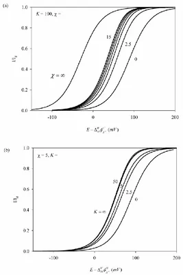
[image:7.596.164.431.281.683.2]The effects of the kinetics and of the equilibrium constant of the complexation reaction in the rigorous NPV response of the FIT are studied in Figure 1. We plot the normalized I/E curves obtained from the rigorous solution (Eq. (8) for 15 and Eq. (18) otherwise) for a fixed value of the equilibrium constant K and different values of the dimensionless kinetic parameter
k1k t2
(Figure 1a) and vice versa (Figure 1b).Figure 1. Normalized rigorous I/E curves, obtained from Eq. (8) for 15 and Eq. (18) for 15, for a fixed value of the equilibrium constant K and different values of the dimensionless
kinetic parameter (Figure 1a) and vice versa (Figure 1b). and K values are given on the curves. DWX 105 cm2 s-1,
8 10 M X
As can be seen, an increase of or K leads to a shift of the rigourous I/E curves to lower potentials, since the ion transfer become easier on account of an enhancement of the ion demand at the organic interface surroundings.
The current varies between two extreme situations with and K:
- Regarding the influence of (Figure 1a), these situations correspond to the case of inert equilibrium ( 0) given by
1 d I e I e (26)
which can be obtained directly from Eq. (8) and is identical to that corresponding to a simple IT [19], and the situation corresponding to total equilibrium conditions (
) given by Eq. (24). Note that small values are the result of organic complexation reactions with slow kinetics, short experiment time, or very low ligand concentration (see Eqs. (15)-(17)), and in constrast, high values can be attributed to fast organic complexation reactions, long experiment durations or very high ligand concentration in the organic phase.- With respect to the influence of K (Figure 1b), the I/E curve shift with this parameter from an equilibrium totally displaced toward the ion (K0), which also correspond to a simple IT (Eq. (26)) to a totally displaced toward the complex equilibrium or irreversible organic complexation (K ). The I/E expression in this last limiting situation can be obtained easily by making K in Eq. (8) and in Eq. (18) for 15,
15 1 2 FIT K K d kss K K d I e S for I e I F otherwise I (27) ,( ) 1 FIT jK j K
j
S a
(28)
1
0
,( ) 0 2 2 2
1 1
; 1
1 ! ( )!
j n
j K j j n
n
e a a
a p p p e p j
e j j n
(29)2 kss
K e
(30)
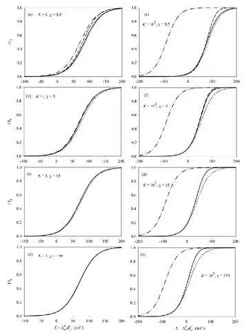
In Figure 2 we compare the rigurous solution (Eq.(8)) with the different approximations. Thus, we have plotted the I/E curves obtained from the rigorous treatment (solid black line) and those of the kss (dash line), dkss (dotted lines) and total equilibrium (dash-dotted lines) approximations for two fixed values of K (K=1 for Figures a-d and K=103 for Figures e-h) and different values of (given on the curves).
Figure 2. Normalized I/E curves corresponding to the rigorous solution (solid lines, obtained from Eq. (8) for 15 and Eq. (18) otherwise), and the kss (dashed lines, Eq. (18)), the dkss (dotted lines, Eq. (21)) and te (dash-dotted lines, Eq. (24)) approximations, for different values of and K(given on the curves). W 10 5
X D
cm2 s-1, M 10 8 X
D
[image:9.596.122.476.175.654.2]
From any of the Figures presented it can be seen immediately that except for very small values of ( = 0.5 in Figures a and e) the kss curves (Eq. (18)) and the rigorous curves (Eq. (8)) practically overlap whatever the K value. Therefore, the kss approximation will be used instead of the rigorous expression for 5.
Regarding the goodness of the dkss and te approximations, it is clear from Figure 2 that their reliability depends on the K and values. In the case of the dkss approximation, we can see that the I/E curves adjusts properly to the rigorous curves for any value when small K values are
considered (K = 1 in Figures a-d); for high K values (K = 103 in Figures e-h) the error in the measurement of the half-wave potentials is as maximum up to of 7 mV (see also Figure 3).
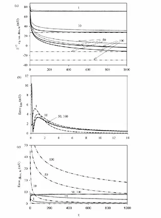
Figure 3. 3a: E1/2 vs curves obtained from the rigorous solution (solid lines, obtained numerically from Eq. (8) for 15 and Eq. (18) otherwise), and from the kss (dashed lines, obtained numerically from Eq. (18)), the dkss (dotted lines, obtained from Eq.(23)) and te (dash-dotted lines, Eq.(25)) approximations, for different values of K(given on the curves). 3b and 3c: Absolute error curves corresponding to the kss (dashed lines), dkss (dotted lines) and te (dash-dotted lines) approximations. wMX0´= 0 mV,
5 10 W X
D cm2 s-1,
8 10 M X
[image:10.596.141.455.241.666.2]
On the other hand, the position of the total equilibrium curves shows a large shift with K with
respect to the rigourous curve in the conditions selected (compare the rigourous and te curves with K =1 and K =103), in such a way that for the range of values selected (0.5 150) the te approximation quickly losses reliability as K increases (see also Figure 3). The error in the
measurement of the half-wave potentials for K=103 is around 100 mV when using this aproximation, so in these conditions the te approximation should not be used.
From these Figures it can be concluded that for relatively small values (0.5 150) the dkss approximation could be used instead of the kss or rigorous one for a general good description of the system, avoiding numerical fitting whatever the K value, whereas the te approximation is only applicable for weak complexes (specifically, for complexes with K15). To obtain more accurate results the kss or rigorous solutions are required.
Figure 3a depicts the evolution of the half-wave potential obtained from the rigorous solution (black solid lines), and from the kss (dashed lines), dkss (dotted lines) and te (dash-dotted lines) approximations with the dimensionless rate constant for a range of values located between 0 and 1000 for different values of the equilibrium constant K (shown on the curves). In order to check the validity of the different approximate solutions in these conditions by comparison with the rigorous results, in Figures 3b and 3c the absolute error of the kss, dkss and te approximations are shown for the different K values selected.
From the rigorous curves depicted in Figure 3a (solid black lines) we can see that E1/2 shifts toward lesser values with and with K, that is, as the metal complex interconversion become faster and as the chemical complexation becomes more irreversible, respectively. With respect to the limiting values taken by E1/2, we can distinguish those corresponding to very slow kinetics or inert equilibrium (0 and/or K0), both of which correspond to the simple ion transfer [19]
1/2 0´ 1
ln W
M X RT E
F
(31)
and also those corresponding to the case of very fast kinetics ( ) and irreversible complexation reactions (K ), which depend on K and , respectively. Indeed, as can be seen from the Figure, for a given K value E1/2 decreases as increases until it reaches the limiting value given by Eq. (25) which depends on K. In the same way, for a given value of E1/2 decreases as K increases until reach its limiting value when the complexation reaction becomes irreversible.
Note that the kss curves in Figure 3a overlap with the rigorous ones except for very small values, and so their differences are not noticeable in the scale selected.
From the error curves presented in Figure 3b we can see that the kss approximation (dashed lines) can be used reliably for 5, since it leads to errors lesser that 1.5 mV (see also the I/E curves presented in Figure 2). Notwithstanding, some precautions must be taken in order to apply dkss and te approximations. From the curves depicted in Figure 3a we can see that, in general, for the different K
(K=1 and 10 in the Figure). Nevertheless, the error in the quantification of E1/2 does not exceed 8 mV for any of the K values presented. With respect to the te approximation, it is totally inadequate to quantify E1/2 within the range of values presented as can be seen for the dash-dotted curves presented in Figure 3a. The error committed with this approximation is much higher than that corresponding to the dkss one, and it increases very quickly with the strength of the complex formed in the organic phase (see the curves in Figure 3c).
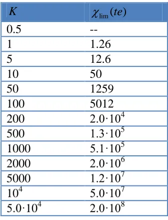
[image:12.596.214.382.300.519.2]The error curve corresponding to the te approximation decays quickly with (see Figure 3c). Table 1 gathers the ( )te lim values above which the te approximation can be used besides the dkss one for a qualitative good description of the system under study, and which correspond to the value above which the difference between E1/2 rigorous and E1/2 approximated is less than 8 mV.
Table 1. values above which the te approximation is applicable.
K lim( )te
0.5 --
1 1.26
5 12.6
10 50
50 1259
100 5012
200 2.0·104
500 1.3·105
1000 5.1·105
2000 2.0·106
5000 1.2·107
104 5.0·107
5.0·104 2.0·108
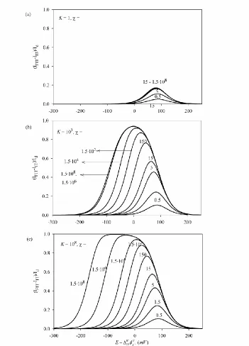
For a given equilibrium constant K, for values lesser than lim( )te the dkss approximation will be always preferable, but for values greater than lim( )te the te expressions (Eqs. (24) and (25) ) can be also used. Bear in mind that for quantitative purposes the rigorous or kss solutions are needed. A good criterion to characterize the existence of complexation in the membrane consists in study the behavior of the difference between the I/E curves obtained in presence and in absence of ligand, so that they present a peak whose height is sensitive to the kinetic and thermodynamic effects of the complexation reaction. Thus, in Figure 4 we present the normalized (IFIT IIT) vs E curves, obtained from Eqs.(8), (18) and (26), for different values of and K (shown on the curves).
coincide for 5, while for moderately strong complexes (K1000 in Figure 4b) the peak height is sensitive to the value up to 106.
Figure 4. Rigorous normalized (IFIT IIT)vs E curves, obtained from Eq. (8) for 15, Eq. (18) for 15
and Eq. (26), for different values of and K (shown on the curves). DWX 10 5
cm2
s-1, DXM 10 8
cm2s-1.
For very high complexation constants (K 108 in Figure 4c) the (IFIT IIT) vs E curves show a plateau with (IFIT IIT) /Id 1 for values higher than
3
[image:13.596.124.475.126.614.2]
complexes (high K values) and fast complexation reactions (high values) the I/E wave corresponding to the FIT appears at much lesser potentials than the simple ion transfer wave, and so the difference between the two normalized I/E signals is equal to the unity.
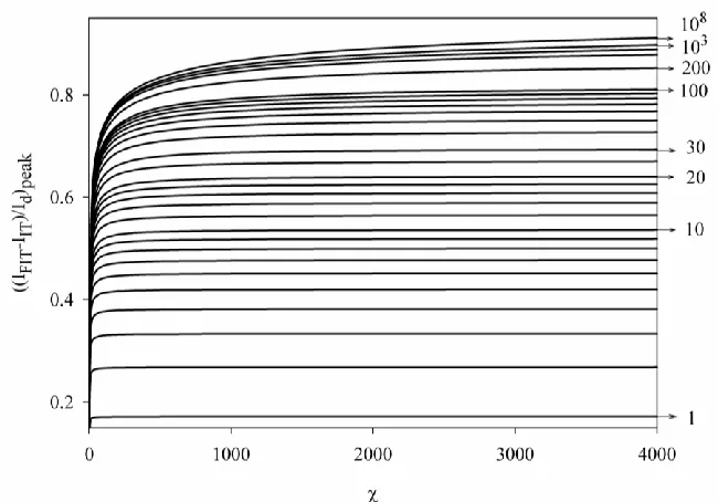
[image:14.596.136.461.205.432.2]The behavior described above suggest the construction of working curves to determinate the kinetic parameters of the system from NPV experiments performed in presence and absence of ionophore in the organic phase, as those presented in Figure 5.
Figure 5.
(IFIT IIT) /Id
peak vs curves obtained from the rigorous solution (Eq. (8) for 15 and Eq. (18) for 15) and Eq. (26) for different K values (given on the curves). wMX0´ = 0 mV,5 10 W X D
cm2 s-1, DXM 10 8
cm2s-1.
From a given K, the value of kinetics of the complexation reaction can be easily obtained from these curves and vice versa. Note that from high and small K values the (IFITIIT) /Id vs curves become insensitive to . This is an indication of the attainment of total equilibrium conditions.
4. CONCLUSIONS
- The influence of the thermodynamic and kinetic parameters
K k1/k2 and k1k2 t
of the complexation reaction on the Facilitated Ion Transfer (FIT)
- The validity of three approximated solutions has been checked by comparison with the rigurous results: the kinetic steady state approximation (kss), the diffusive kinetic steady state aproximation (dkss), and the total equilibrium aproximation (te). From this comparison we have pointed out that the kss aproximation can be reliably used instead of the rigorous one for any K value when
k1k t2
5. Moreover, with respect to the more severe dkss and te approximations, the dkss treatment can be used instead of the rigorous solution for a reasonably good qualitative description of the system for any value of and K values, not involving errors greater than 8 mV. However the te treatment is only applicable for fast organic complexation reactions and weak complexes (see Table 1). - It is shown that the existence of complexation in the membrane can be characterized by studying the behavior of the difference between the I/E curves obtained in presence and in absence of ligand on account of the fact that they present a peak of which height is sensitive to the kinetic and thermodynamic effects of the complexation reaction. In this respect, working curves have been proposed to determine the forward and backward kinetic constants of the complexation reaction based on these differences.ACKNOWLEDGEMENTS
The authors greatly appreciate the financial support provided by the Dirección General de Investigación Científica y Técnica (Project Numbers CTQ2011-27049/BQU and CTQ2009-13023/BQU), and the Fundación SENECA (Project Number 08813/PI/08). Also, E. T. thanks the Ministerio de Ciencia e Innovación for the grant received.
References
1. Z. Samec, Pure Appl. Chem., 76 (2004) 2147.
2. A. Molina, C. Serna, J. A. Ortuño and E. Torralba, Annu. Rep. Prog. Chem., Sect. C, 108 (2012) 126.
3. R. Gulaboski, E. S. Ferreira, C. M. Pereira, M. N. D. S. Cordeiro, A Garau, V. Lippolis and A. F. Silva, J. Phys. Chem. C, 112 (2008) 153.
4. J. Langmaier and Z. Samec, Anal. Chem. 81 (2009) 6382. 5. S. A. Dassie, J. Electroanal. Chem, 643 (2010) 20.
6. F. Reymond, P. Carrupt and H. H. Girault, J. Electroanal. Chem., 449 (1998) 49. 7. M. M. Faul and B. E. Huff, Chem. Rev., 100 (2000) 2407.
8. P. Bühlmann, E. Pretsch and E. Bakker, Chem. Rev., 98 (1998) 1593. 9. Z. Samec, E. Samcová and H. H. Girault, Talanta, 63 (2004) 21.
10.M. Senda, H. Katano and M. Yamada, J. Electroanal. Chem., 468 (1999) 34. 11.J. Koryta, Electrochim. Acta, 24 (1978) 293.
12.H. Wang, N. Liu , L. Xi, X. Rong, J. Ruan, and Y. Huang, Appl. Environ. Microbiol., doi:10.1128/AEM.02915-10.
16.A. Molina, I. Morales and M. Lopez-Tenes, Electrochem. Commun., 8 (2006) 1062. 17.A. Molina and I. Morales, Electrochem. Commun., 8 (2006) 1453.
18.H. Matsuda, Y. Kamada, K. Kanamori, Y. Kudo and Y. Takeda, Bull. Chem. Soc. Jpn., 64 (1991) 1497.
19.A. Molina, C. Serna, J. A. Ortuño and E. Torralba, Int. J. Electrochem. Sci., 3 (2008) 1081.