A formal sensitivity analysis for Laguerre based predictive functional control

This is a repository copy of

A formal sensitivity analysis for Laguerre based predictive

functional control

.

White Rose Research Online URL for this paper:

http://eprints.whiterose.ac.uk/133017/

Version: Accepted Version

Proceedings Paper:

Abdullah, M. and Rossiter, J.A. (2018) A formal sensitivity analysis for Laguerre based

predictive functional control. In: Proceedings of 2018 UKACC 12th International

Conference on Control (CONTROL). Control 2018: The 12th International UKACC

Conference on Control, 05-07 Sep 2018, Sheffield, UK. IEEE , pp. 20-25. ISBN

978-1-5386-2864-5

https://doi.org/10.1109/CONTROL.2018.8516849

© IEEE 2018. Personal use of this material is permitted. Permission from IEEE must be

obtained for all other users, including reprinting/ republishing this material for advertising or

promotional purposes, creating new collective works for resale or redistribution to servers

or lists, or reuse of any copyrighted components of this work in other works. Reproduced

in accordance with the publisher's self-archiving policy.

[email protected] https://eprints.whiterose.ac.uk/

Reuse

Items deposited in White Rose Research Online are protected by copyright, with all rights reserved unless indicated otherwise. They may be downloaded and/or printed for private study, or other acts as permitted by national copyright laws. The publisher or other rights holders may allow further reproduction and re-use of the full text version. This is indicated by the licence information on the White Rose Research Online record for the item.

Takedown

If you consider content in White Rose Research Online to be in breach of UK law, please notify us by

A Formal Sensitivity Analysis for Laguerre Based

Predictive Functional Control

Muhammad Abdullah

and John Anthony Rossiter

∗†_{Department of Automatic Control and System Engineering,}

University of Sheffield, Mappin Street, S1 3JD, UK.

Email: [email protected]∗ and [email protected]†

∗_{Department of Mechanical Engineering,}

International Islamic University Malaysia, Jalan Gombak, 53100, Kuala Lumpur Malaysia. Email: mohd [email protected]∗

Abstract—A Laguerre Predictive Functional Control (LPFC) is a simple input shaping method, which can improve the prediction consistency and closed-loop performance of the conventional approach (PFC). However, it is well-known that an input shaping method, in general, will affect the loop sensitivity of a system. Hence, this paper presents a formal sensitivity analysis of LPFC by considering the effect of noise, unmeasured disturbance and parameter uncertainty. Sensitivity plots from bode diagrams and closed-loop simulation are used to illustrate the controller robustness and indicate that although LPFC often provides a better closed-loop tracking response and disturbance rejection, this may involve some trade-off with the sensitivity to noise and parameter uncertainty. Finally, to validate the practicality of the results, the sensitivity of the LPFC control law is illustrated on real-time laboratory hardware.

Index Terms—Predictive Control, PFC, Sensitivity Analysis, Laguerre function, Parameter Uncertainty, Noise, Disturbance

I. INTRODUCTION

Model Predictive Control (MPC) is an optimal controller that employs a control action based on a future output pre-diction. Typically, MPC utilises a finite horizon prediction in the optimisation process and can explicitly take into account different types of constraints in a system [1]. Nevertheless, the implementation of this controller is often more expensive and requires higher computational effort and time compared to its competitors [2]. Hence for low-end applications, it is wiser to consider a simpler controller such as Proportional Integral Derivative (PID) or Predictive Functional Control (PFC).

Developed in 1973, PFC is known as a simplified version of MPC that minimises the output error at a single point instead of over a whole trajectory [3], [4]. With this simplification, PFC only needs simple coding and minimal computation. Although in general, the computed input is not optimal, it still retains some of the core benefits of an MPC approach such as systematic handling of constraints and/or systems with delays [4]. Besides, the use of a target first-order Closed-loop Time Response (CLTR) as one of its tuning parameters, makes the design process more transparent. Currently, this controller is widely used in many industrial applications and has become a prime competitor with PID regulators [4]–[6].

This work is funded by International Islamic University Malaysia and Ministry of Higher Education Malaysia.

Despite its attractive attributes, the simple PFC concept is often unable to provide a consistent prediction [7], accurate constrained solutions [8] and effective handling of systems with challenging dynamics [9], [10]. Several works have mod-ified the traditional PFC framework to tackle these weaknesses either via cascade structures [4], [11], pole-placement [9], [12] or input shaping [8], [10]. However, the derivation of these methods often excludes explicit consideration of uncer-tainty, and only a few works have systematically discussed or analysed the robustness of PFC [13], [14]. Hence, the main objective of this work is to tackle this issue on one of its alternative structures know as Laguerre PFC (LPFC).

LPFC is defined by shaping the future predicted input trajec-tory with a first-order Laguerre polynomial [15], [16]. Instead of the constant input assumption of PFC, the future dynamics are now forced to converge gradually to the steady-state value. This modification can improve the prediction consistency and the significance of CLTR as a tuning parameter [16]. Furthermore, due to the well-posed decision making, satisfying constraints within a larger validation horizon becomes more accurate and less conservative [8]. However, this algorithm, as in common in MPC, is utilising the model parameters to estimate the steady state input while improving the loop performance and hence, it is worth investigating its sensitivity concerning noise, disturbances and parameter uncertainty.

Since the general unconstrained PFC framework provides a fixed control law, loop sensitivity can be computed and analysed to assess the controller robustness [3]. The perfor-mance of LPFC will be benchmarked against a nominal PFC structure to get some insight into the sort of sensitivity trade-off that ones should expect. The reader is reminded again that the scope of this work is only focused on simple and stable dynamic system; further development of LPFC to deal with challenging or unstable systems constitutes future work and in general is non-simple with a PFC approach.

II. PFC STRUCTURES ANDSENSITIVITYFUNCTIONS

This section presents a brief formulation for both PFC and LPFC together with the derivation of their sensitivity functions. More detailed derivations, theory and concepts are available in these references [3], [4], [6], [7]. Without loss of generality, this work utilises an autoregressive with exogenous terms (ARX) model with an independent model (IM) structure.

A. Conventional PFC

1) Target trajectory: PFC is designed to follow a

closed-loop behaviour of the first order system with a delay τ (or h

samples) and a time constant Tr [7]. The z-transform of the

target trajectory,r(z)with steady-stateR is:

r(z) =z

−h_(1−λ)

1−λz−1 R (1)

The representation of target pole,λin (1) is equivalent to the desired closed-loop time response (CLTR) which is normally used by industrial practitioners [4]. The conversion can be presented by Tr = CLT R/3, where λ = e

−T

T r with T the

sampling period.

2) Coincidence point and degree of freedom: The control

objective of PFC is to force the system open-loop prediction,

yp to exactly match the predicted target trajectory of (1) at

a selected coincidence point n samples into the future [4]. Consequently, the control law is formulated to enforce the equality:

yp,k+n|k= (1−λn)R+λnyp,k (2)

where yp,k+n|k is the n-step ahead system prediction at

sample time k and yp,k is the current process output

measurement.

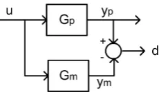
3) Independent model: The independent model (IM)

struc-ture is often used in conventional PFC [4], [5] as this is known to provide good sensitivity properties in general, yet it is only applicable to open-loop stable systems. The implemen-tation is equivalent to using a step response model (ignoring truncation errors [1]). Both the model Gm and process Gp

run in parallel using the same input uk (see Fig.1). The

error (dk = yp,k −y_m,k) between process output y_p and

model output ym is utilised to handle noise, disturbance and

parameter uncertainty. Using the unbiased model prediction, the equality (2) is altered to:

(1−λn)R+λny_p,k =y_m,k+n|k+d_k

(R−y_p,k)(1−λn) =y_m,k+n|k−y_m,k (3)

4) Control law: The n-step ahead prediction algebra for

an ARX model is well known in the literature, which can be represented using Toeplitz/Hankel form (e.g. [1]), hence only the final form is given here. For inputuk and model outputs

ym,k, the n-step ahead linear prediction model is:

ym,k+n|k=Huk

→ +P u←k+Qym,k← (4)

Fig. 1: The independent model structure.

where parameters H, P, Qdepend on the model parameters and for a model of order m:

u_→k=



   

uk uk+1

.. .

uk+n−1 

   

; u_←k=



   

uk−1 uk−2

.. .

uk−m



   

; ym,k

← = 

   

ym,k ym,k−1

.. .

ym,k−m



   

(5)

Substituting prediction (4) into equality (3) gives:

Huk

→+P u←k+Qym,k← −ym,k= (R−yp,k)(1−λ

n₎

(6)

The constant future input assumption of PFC [3], [4] means that uk+i|n =uk for i >0, hence defining h=P(H), the

control law reduces to:

uk =

1

h

(1−λn)R−(1−λn)y_p,k−Qym,k

← +ym,k−P u←k

(7)

The control law can be represented in a vector form by rearranging (7) in terms of parameters Fp, Np, Mp and Dˆp

with obvious definitions:

uk =FpR−Npym,k

← −Mpyp,k−Dˆp∆←uk (8)

Remark 1: Conventional PFC can work well with low

order and simple dynamical systems, especially when the coincidence point is selected properly [7]. However, with the restricted degree of freedom (d.o.f) in its future input dynamics, an inconsistency between open-loop and closed-loop predictions will occur [7], [16]. Since the current decision making could then be ill-posed, the accuracy of a constrained solution might also be affected, especially when the validation horizon is selected far beyond the coincidence point [8].

B. Laguerre based PFC (LPFC)

1) Future input dynamics: The main difference between

LPFC and PFC is that the future predicted input dynamics are shaped via a first-order Laguerre polynomial (in effect, a simple exponential decay function with pole a) so that it will converge to the expected steady state input uss [15], [16].

Thus, instead of the constant dynamics assumption of PFC, the future input is modified to

uk

→ =uss+Lη (9)

where L is the vector (L = [1, a, a2_{, ...a}n−1_]T_{) and η is a}

degree of freedom. For a general transfer function Gm(z) =

B(z)A(z)−1_{, the value u}

ss is estimated as:

uss=Gm(z)−1(R−dk) (10)

The inclusion of error termdk in (10) is to ensure an unbiased

Remark 2: For a first-order system, a should be equal to

λ to ensure consistent dynamics with the target trajectory [16]. Although for higher-order systems, the value of a can be tuned for faster convergence [15], this work will only use

a=λto keep the sensitivity analysis transparent.

2) LPFC control law: The output prediction of (4) is

modified with the new input dynamics of (9) to give:

ym,k+n|k =H(uss+Lη) +P uk

←+Qym,k← (11)

The equality of (6) now becomes:

HLη+huss+P uk

←+Qym,k← −ym,k= (r−yp,k)(1−λ

n₎

(12)

and the control law is computed by solving forη as:

η= 1

HL

(1−λn)r−(1−λn)y_p,k−hu_ss−Qym,k

← +ym,k−P u←k

(13) Due to the receding horizon principle [3] and the definition of

L(z), the current input is defined as:

uk =uss+η (14)

Noting the structure of uss in (10) and η in (13), the

manipulated inputuk in (14) can be altered into vector form

simply by rearranging the algebra and grouping the common terms into parameters Fl,Nl,Ml andDˆl so that:

uk=Flr−Nlym,k

← −Mlyp,k−Dˆl∆←uk (15)

Remark 3:It has been shown in [16] that LPFC law of (15)

manages to improve the prediction consistency and the efficacy of λ as tuning parameter compared to the conventional PFC law of (8). In addition, the constrained solution becomes more accurate and less conservative [8].

C. General Sensitivity function for IM structure

From the previous subsections, it is clear that both PFC and LPFC can be represented by a fixed control law as in (8) and (15). These are used in the derivation of sensitivity functions presented next to analyse their respective robustness [1].

First consider a generic formulation of the control law within an IM structure:

uk=F r−N ym,k

← −M yp,k−Dˆ∆←uk (16)

This can be represented in a transfer function form, where the vectors of

N = [N0, N1, N2, ..., Nn]

ˆ

D= [ ˆD0,Dˆ1,Dˆ2, ...,Dˆn]

(17)

are defined in thez domain as:

N(z) =N0+N1z−1, N2z−2+...+Nnz−n

ˆ

D(z) = ˆD0+ ˆD1z−1,Dˆ2z−2+...+ ˆDnz−n

D(z) = 1 +z−1Dˆ(z)

(18)

Noting the definitions of uk

← andym,k← in (5), the sensitivity

functions are derived based on a closed-loop form of:

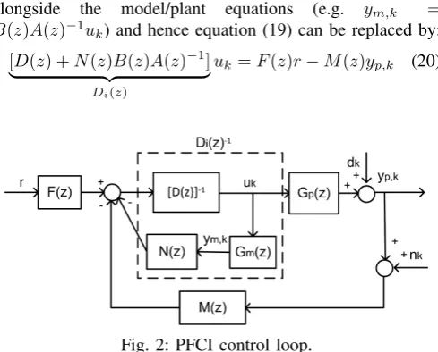
D(z)uk=F(z)r−N(z)ym,k−M(z)yp,k (19)

alongside the model/plant equations (e.g. ym,k =

B(z)A(z)−1_u

k) and hence equation (19) can be replaced by:

[D(z) +N(z)B(z)A(z)−1]

| {z }

Di(z)

uk=F(z)r−M(z)y_p,k (20)

Fig. 2: PFCI control loop.

Fig. 2 indicates the equivalent block diagram with the addition of measurement noise nk and output disturbance

dk. From the structure, the effective control law can be

simplified to K(z) = M(z)[Di(z)∆]−1. Assuming

sys-tem G(z) = B(z)A(z)−1_{, the closed-loop pole polynomial}

Pi(z) = 1 +K(z)G(z)is represented as:

Pi(z) =Di(z)A(z) +M(z)B(z) (21)

The sensitivity of the input to noise is derived by finding the transference fromn(z)tou(z)(refer to Fig. 2):

Sun=K(z)[1 +K(z)G(z)]−1=M(z)Pi(z)−1A(z) (22)

Similarly, the sensitivity of output to disturbance is obtained by solving the transference from d(z)toy(z):

Syd= [1 +K(z)G(z)]−1=A(z)Pi(z)−1Di(z) (23)

Finally, the multiplicative uncertainty is modelled as G(z)→

(1 +δ)G(z), for δ a scalar (possibly frequency dependent). Thus the closed-loop pole sensitivity to multiplicative uncer-tainty becomes:

Pc = [1 +G(1 +δ)K] = 0

Sg =GK[1 +K(z)G(z)]−1=M(z)Pi(z)−1B(z)

(24)

D. Summary of Control Laws

Table I summarises some of the sensitivity functions for PFC and LPFC. It is noted that the structures of all the sensitivity functions are same, but obviously with different parameters and hence, different sensitivity responses should be expected.

TABLE I: Sensitivity functions for PFC and LPFC.

Algorithm PFC LPFC

S_un M_p(z)P_i,p(z)−1A(z) M_l(z)P_i,l(z)−1A(z)

S_yd A₍z₎P_i,p(z₎−1D_i,p(z₎ A₍z₎P_i,l(z₎−1D_i,l(z₎ S_g M_p(z₎P−1

i,pB(z) Ml(z)Pi,l−1B(z)

The polynomials M(z), D(z), Pi(z)used a subscriptpfor

III. NUMERICAL EXAMPLES

This section presents the sensitivity analysis of uncon-strained second order over-damped process (25) as constraint handling would imply non-linear control. In fact, if the loop structure has low sensitivity in the nominal case, it is likely to carry over for the constrained case. For the first example, both PFC and LPFC are tuned using a fasterλcompared to the slowest open-loop pole. The second example demonstrates the effect of loop sensitivity when the controllers are tuned to have almost similar closed-loop poles. The outcome of this analysis is then validated with the closed-loop simulation using Matlab.

G1=

0.1z−1_{+ 0.4z}−2

(1−0.5z−1)(1−0.9z−1) (25) A. First example

10-2 10-1 100 101

Frequency 10-2

10-1 100

Closed-loop bandwidth

PFC LPFC

10-2 10-1 100 101

Frequency 10-2

100 102

Output sensitivity to disturbances

10-2 10-1 100 101

Frequency 0.2

0.3 0.4

Input sensitivity to measurement noise

10-2 10-1 100 101

Frequency 10-2

10-1 100

Sensitivity to multiplicative uncertainty

Fig. 3: Sensitivity plot for processG1withλ= 0.7andn= 7.

In this example, the system (25) is considered to track a unit set point. The desired pole is set to λ= 0.7, while the coincidence point is tuned atn= 7using conjecture presented in [7], that is corresponding to 40% to 80% rise of the step response to the steady-state value.

To analyse the trade-off between performance and robust-ness of PFC and LPFC, the Bode plots of each sensitivity function are plotted together with their closed-loop bandwidth (see Fig. 3). It can be observed that:

• for this particular selection of tuning parameters, LPFC (red dotted line) has a higher bandwidth compared to PFC (blue dashed line). Since LPFC has a faster dynam-ics, it becomes less sensitive in rejecting low-frequency disturbance..

• However, higher bandwidth requires more aggressive

input activity, and thus LPFC becomes more sensitive to measurement noise and modelling uncertainty compared to conventional PFC.

One could argue that PFC has failed to deliver the desired bandwidth and if LPFC were to be tuned to give an equivalent

lower bandwidth, in all likelihood, the sensitivities would be similar.

0 20 40 60

Samples -0.5

0

0.5 Input with disturbance

0 20 40 60

Samples 0

0.5 1 1.5

2 Output with disturbance

0 20 40 60

Samples 0

0.1 0.2 0.3

0.4 Input with noise

0 20 40 60

Samples 0

0.5 1

Output with noise

0 20 40 60

Samples 0

0.1 0.2 0.3

0.4 Input with uncertainty

0 20 40 60

Samples 0

0.5 1

Output with uncertainty

Target trajectory LPFC PFC

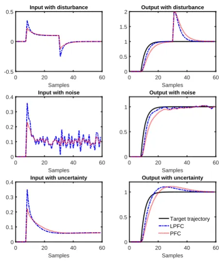
Fig. 4: Closed-loop response of processG1withλ= 0.7and

n= 7in the presence of disturbance, noise, and uncertainty. To validate this analysis, a closed-loop control (see Fig. 4) is simulated with three different conditions:

1) A step output disturbance (d= 1) is added to the 30th sample.

2) The output measurement is corrupted by Gaussian ran-dom white noise with variance of 0.1.

3) SystemG1,m(26) is used to predict the future dynamics

instead ofG1 to demonstrate the effect of uncertainty.

G1,m=

0.12z−1_{+ 0.37z}−2

1−1.37z−1+ 0.4z−2 (26)

The simulation outcomes reflect the previous sensitivity anal-ysis whereby:

• LPFC converges approximately 2 samples faster in track-ing the target and rejecttrack-ing the output disturbance with almost similar overshoot (ymax= 2) compared to PFC. • On the other hands, LPFC reacts more to the noise in the

input compared to conventional PFC.

• For parameter uncertainty, both controllers manage to converge towards the steady-state value but with apparent differences in their closed-loop response.

poles with LPFC delivering the desired pole and PFC not doing so.

10-2 10-1 100 101

Frequency 10-2

10-1

100 Closed-loop bandwidth

PFC LPFC

10-2 10-1 100 101

Frequency 0.2

0.4 0.6 0.8 1

Output sensitivity to disturbances

10-2 10-1 100 101

Frequency 10-2

10-1 100

Input sensitivity to measurement noise

10-2 10-1 100 101

Frequency 10-2

10-1 100

Sensitivity to multiplicative uncertainty

Fig. 5: Sensitivity plot for process G1 with λ = 0.92 and

n= 9.

B. Second example

The next example looks at the effect of sensitivity when the process (25) is tuned using slowerλ = 0.92 (almost similar with the slowest open-loop pole). Based on the same procedure [7], the coincidence pointn= 9is selected to track a unit set point. It can be observed that (see Fig. 5):

• With the selected tuning parameters, LPFC and PFC have almost a similar bandwidth.

• As a consequence, both controllers are giving a close sensitivity outcome with respect to disturbance, noise and modelling uncertainty.

Again to validate the sensitivity analysis, the closed-loop simulation is run to track a unity set point for three different cases (similar as previous example). The outcomes in Fig. 6 demonstrates that:

• PFC and LPFC converge at the same rate and very close to the target trajectory while rejecting the disturabce with overshoot approximately aroundymax= 1.8.

• Similar observation can be seen with the presence of

noise and modelling uncertainty where both controllers performance are almost same.

C. Summary

In summary, for the two cases given, the controller sensi-tivity is related to the achieved closed-loop bandwidth. LPFC is better at delivering the target λ whereas PFC often gives a slower response than desired when large n is required. In consequence, for the same λ, LPFC is usually more highly tuned and thus more sensitive to noise and modelling un-certainty. However, where the two control laws give similar closed-loop poles (perhaps by deploying different λ), their

0 20 40 60 80

Samples -0.05

0 0.05 0.1

0.15 Input with disturbance

0 20 40 60 80

Samples 0

0.5 1 1.5

2 Output with disturbance

0 20 40 60 80

Samples 0

0.05 0.1

0.15 Input with noise

0 20 40 60 80

Samples 0

0.2 0.4 0.6 0.8 1

Output with noise

0 20 40 60 80

Samples 0

0.02 0.04 0.06 0.08 0.1

Input with uncertainty

0 20 40 60 80

Samples 0

0.2 0.4 0.6 0.8 1

Output with uncertainty

Target trajectory LPFC PFC

Fig. 6: Closed-loop response of processG1withλ= 0.92and

n= 9in the presence of disturbance, noise and uncertainty.

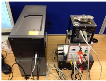
Fig. 7: Quanser SRV02 servo based unit.

sensitivities are similar. Therefore, LPFC is a better base on which to explore the trade-offs in the sensitivity, as there is a stronger connection between the tuning parameters and the achieved closed-loop performance [16] in addition to a better constraint handling due to its well-posed decision and prediction consistency as discussed in [8].

IV. REALTIMESYSTEMIMPLEMENTATION

0 1 2 3 4 Time (s)

-0.5 0 0.5 1 1.5

Input voltage (V)

Step input

0 1 2 3 4

Time (s) 0

0.5 1 1.5 2

Angular speed (rad/s)

Open-loop response

y_m

y p

0 1 2 3 4

Time (s) -0.5

0 0.5 1 1.5

Input voltage (V)

Control input

0 1 2 3 4

Time (s) -1

0 1 2

Angular speed (rad/s)

LPFC closed-loop response

Target y

p

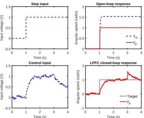
Fig. 8: Step response and LPFC closed-loop behaviour for processG2.

is run by National Instrument LabVIEW software via USB connection (see Fig. 7). The objective is to track the desired servo angular speed, θ˙(t) by regulating the supplied voltage,

V(t). The mathematical model is given as [17]:

0.0254¨θ(t) = 1.53V(t)−θ˙(t) (27)

where θ¨(t) is the servo angular acceleration. Converting the model (27) to discrete form with sampling time 0.02s, the transfer function of angular speed to voltage input becomes:

G2=

0.8338

1−0.455z−1 (28)

The upper Fig. 6 shows the modelling uncertainty between the processyp and modelymsubjected to a step inputu. To track

the angular speed at 1 rad/s, LPFC is tuned withn= 1(often a sensible choice for a first-order system [7]) with desired CLTR at0.5s(equivalent to λ= 0.89). It is noted that at3s, there is a step output disturbance (d= 2) entering the system while the measurement is corrupted by Gaussian white noise with variance of 0.5. The closed-loop response (see lower Fig. 8) shows that:

• LPFC manages to reduce some noise transmission to the input with approximate 0.2 variance from 0.5, while rejecting the output disturbance.

• Although there is modelling uncertainty, the selected CLTR is still achieved at0.5swith minimum offset error.

V. CONCLUSIONS

This work provides a formal sensitivity analysis of LPFC in the presence of noise, disturbance and modelling uncertainty. The performance is then compared with the conventional PFC control law. Indeed it is clear that when using LPFC, a user need to pay a small trade-off by having a more sensitive controller to noise and uncertainty since it is highly tuned with a larger bandwidth than conventional PFC. However, both

controllers may typically have similar sensitivities if giving similar closed-loop poles which would indicate a preference for LPFC in general due to easier tuning and other advantages as discussed inRemark 3.

Future work will consider the analysis of different PFC structures that deal with more challenging dynamics and unstable systems as PFC is currently has a number of ad-hoc constructive methods to improve its closed-loop behaviour. In addition, a core issue that also needs to be considered is the impact of modelling assumptions on sensitivity. This paper assumes an IM model of Fig. 1, so it would be interesting to consider how sensitivity might change with alternative prediction models such as T-filter [14].

ACKNOWLEDGMENT

The first author would like to acknowledge International Islamic University Malaysia and Ministry of Higher Education Malaysia for funding this work.

REFERENCES

[1] J. A. Rossiter, Model predictive control: a practical approach, CRC Press, 2003.

[2] L. G. Bleris and M. V. Kothare, “Real-Time implementation of Model Predictive Control,” American Control Conference, Portland, USA, 2015.

[3] J. Richalet, A. Rault, J.L. Testud and J. Papon, Model predictive heuristic control: applications to industrial processes,Automatica, 14(5), 413-428, 1978.

[4] J. Richalet, and D. O’Donovan,Predictive Functional Control: princi-ples and industrial applications. Springer-Verlag, 2009.

[5] J. Richalet, and D. O’Donovan, “Elementary Predictive Functional Control: a tutorial,” Int. Symposium on Advanced Control of Industrial Processes, 2011, pp. 306-313.

[6] R. Haber, J.A. Rossiter and K. Zabet, “An Alternative for PID control: Predictive Functional Control - A Tutorial,” American Control Confer-ence (ACC), 2016, pp. 6935-6940

[7] J. A. Rossiter, and R. Haber, “The effect of coincidence horizon on predictive functional control,”Processes, 3, 1, pp. 25-45, 2015. [8] M. Abdullah, J. A. Rossiter and R. Haber, “Development of constrained

predictive functional control using laguerre function based prediction,” IFAC World Congress, 2017.

[9] J. A. Rossiter, R. Haber, and K. Zabet, “Pole-placement predictive functional control for over-damped systems with real poles”,ISA Trans-actions, vol. 61, pp. 229-239, 2016.

[10] J. A. Rossiter, “Input shaping for PFC: how and why?,”J. Control and Decision, pp. 1-14, Sep. 2015.

[11] M. Khadir and J. Ringwood, “Extension of first order predictive func-tional controllers to handle higher order internal models,Int. Journal of Applied Mathematics and Comp. Science, vol. 18, no. 2, pp. 229-239, 2008.

[12] K. Zabet, J. A. Rossiter, R. Haber, and M. Abdullah, “Pole-placement Predictive Functional Control for under-damped systems with real num-bers algebra”,ISA Transactions, In Press., 2017.

[13] K. Zabet and R. Haber, “Robust tuning of PFC (Predictive Functional Control) based on first- and aperiodic second-order plus time delay models”,Journal of Process Control, vol. 54, pp. 25-37, 2017. [14] M. Abdullah and J. A. Rossiter, “The effect of model structure on

the noise and disturbance sensitivity of Predictive Functional Control”, under review for European Control Conference, 2018.

[15] M. Abdullah and J. A. Rossiter, “Alternative Method for Predictive Functional Control to Handle an Integrating Process”, under review for Advances in PID, 2018.

[16] M. Abdullah and J. A. Rossiter, “Utilising Laguerre function in predic-tive functional control to ensure prediction consistency,” 11th Int. Conf. on Control, Belfast, UK, 2016.