Frequency Tuning Range Control in Pulsed Terahertz Quantum Cascade Lasers: Applications in Interferometry

Abstract— Terahertz quantum cascade-lasers (QCLs) are able to produce higher optical output power at higher temperatures when operated in pulsed mode. Predicting a laser’s behav-ior under pulsed operation in order to achieve performance requirements is, however, a nontrivial exercise: the complex and nonlinear interplay between current, electric field, and thermal transients gives rise to complex responses in both optical output power and emission frequency. In applications where it is important to predict and control these behaviors, establishing the link between current drive, emission frequency, and optical output power is necessary. In this paper, we demonstrate, via a realistic laser-specific model, that by appropriate manipulation of the drive pulse we can not only obtain a higher optical output at increased operating temperature but also both extend and linearize a QCL’s frequency sweep. We suggest that consideration of laser behavior through realistic and comprehensive modeling is not only useful but is also required in any pulsed application in which emission frequency change is likely to affect performance.

Index Terms— Quantum cascade laser, rate equation model, laser feedback interferometry, adiabatic frequency modulation, thermal frequency modulation.

I. INTRODUCTION

T

Manuscript received December 7, 2017; revised January 29, 2018; accepted February 6, 2018. Date of publication February 23, 2018; date of cur-rent version March 2, 2018. This work was supported in part by the Australian Research Council’s Discovery Projects Funding Scheme under Grant DP 160 103910, in part by the Queensland Government’s Advance Queensland Programme, in part by the EPSRC, U.K., through DTG Award under Grant EP/J017671/1 and Grant EP/J002356/1, in part by the Royal Soci-ety through the Wolfson Research Merit Awards under Grant WM110032 and Grant WM150029, and in part by the European Cooperation in Science and Technology under Grant BM1205 and Grant MP1406. (Corresponding author:

Aleksandar D. Raki´c.)

G. Agnew, K. Bertling, Y. L. Lim, and A. D. Raki´c are with the School of Information Technology and Electrical Engineering, The University of Queensland, Brisbane, QLD 4072, Australia (e-mail: [email protected]).

A. Grier, Z. Ikoni´c, P. Dean, A. Valavanis, and D. Indjin are with the School of Electronic and Electrical Engineering, University of Leeds, Leeds LS2 9JT, U.K.

T. Taimre is with the School of Mathematics and Physics, The University of Queensland, Brisbane, QLD 4072, Australia

This paper has supplementary downloadable material available at http:// ieeexplore.ieee.org (File size: 313 KB).

Color versions of one or more of the figures in this paper are available online at http://ieeexplore.ieee.org.

Digital Object Identifier 10.1109/JQE.2018.2806948

choice [1]. Terahertz QCLs are now able to source up to 1 W in pulsed mode [2] and operate at temperatures as high as 200 K in pulsed mode [3]. Problems with operating temperature in mid infrared (MIR) QCLs have been largely overcome but remain for THz QCLs [4], [5]: to-date, cryostats are a necessity for THz QCL operation. Pulsed, as opposed to continuous wave (cw), operation of THz QCLs makes it possible to achieve significantly higher optical power outputs at higher ambient temperatures [6]–[8], potentially making it possible to use a liquid nitrogen instead of helium cryostat. The advantages of pulsed operation have led to its widespread use. Pulsed mode operation comes at a cost, however. In cw, a laser’s lattice temperature is for practical purposes con-stant, and therefore does not usually require consideration. When pulsed, bursts of heat created by the excitation cur-rent give rise to large temperature transients in the laser’s active region [9]–[12]. Since the operating state of a QCL is temperature-dependent [13]–[15], these transients have a significant effect on the laser’s behavior, including its emission frequency. Moreover, there is an interplay in the dynamics produced by current and temperature change — simultane-ously changing drive current and lattice temperature thus markedly increases the complexity of device behavior [16]. To realize an efficient and effective application, predicting and understanding this complexity is necessary at the design phase. Due to the nonlinear interplay between lattice temperature, drive current, and photon and carrier numbers, the dynamic behavior of pulsed QCLs [17]–[20] is non-intuitive and cannot be predicted or estimated with simple pencil-and-paper calculations — accurate rate equation modeling is thus an important tool for understanding the complex behavior of pulsed QCLs. This is especially true in laser feedback interferometry (LFI) [21], where the detected signal depends intimately on not only the laser’s behavior, but also on emitted radiation that is reflected back into the laser’s cavity [22].

In this paper we use an accurate reduced rate equa-tion (RRE) model of a real exemplar THz QCL under optical feedback to explore swept-frequency LFI in the pulsed regime. We show that the advantages of pulsed operation can be realized in swept-frequency LFI sensors and that a significant challenge introduced by pulsing, viz. the strongly nonlinear swept-frequency component it creates, can be corrected and

Fig. 1. Model of a pulsed QCL under optical feedback (color online). The behavior of the laser depends on externally imposed conditions, viz. the drive current, cold finger (operating) temperature and external cavity characteristics, as well its internal state which includes its lattice temperature.

moreover, turned to advantage by using it to extend the range of a laser’s frequency sweep. Via the model, we study the QCL’s response to pulsing, offer an approach to finding the timescale that provides maximum frequency sweep, and show that by applying a pre-emphasis component to drive current the thermal nonlinearity in a sweep can be completely nulled. This work is an important step in providing a highly linear frequency sweep in our laboratory LFI work that includes imaging, standoff imaging, and refractive index measurement of materials at THz frequencies.

In section II we introduce pulsed LFI as the context of this research and describe the realistic model of a QCL used to arrive at our results. In section III we present results obtained using three types of linear sweep drive pulse. We then describe the derivation of a current drive pre-emphasis function that corrects the nonlinearity in frequency sweep introduced by its thermal component. In section IV we provide some concluding remarks about the applicability and scope of the combined modulation method.

II. BACKGROUND ANDMODELINGMETHOD Of the many materials analysis and imaging techniques now routinely being used at THz frequencies, LFI is particularly elegant, as the laser functions both as source and detector [23]. The basic LFI configuration is illustrated in Fig. 1. The self-mixing (SM) signal [24], [25] carries information about the target which can be revealed with appropriate processing. A particularly useful class of LFI sensing is “swept-frequency LFI” [26]. Sweeping a laser’s emission frequency produces an interferogram from which target information such as position, complex reflectivity and refractive index, can be inferred. Improved LFI results can be obtained with larger frequency changes, making techniques for extending the range of a laser’s frequency sweep sought after.

To date, frequency modulation has been accomplished almost exclusively via the adiabatic mechanism, in which the laser is operated in cw and small linear variations in drive current superimposed on a DC bias current. The superimposed waveform is typically a sawtooth, producing a repeating, reasonably linear frequency sweep, illustrated in

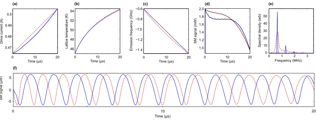
Fig. 2. Self-mixing in a pulsed QCL under optical feedback (color online). Red/broken lines pertain to cw operation and blue/solid lines to pulsed operation. Part (a) shows linear drive current ramps in each mode, with (i) denoting the start of the ramp and (ii) the end. Temperature transients resulting from self-heating are shown in (b). Cold finger temperature in cw is well below that in pulsed mode, in order for results to be comparable. The traces in (c) are emission frequency change resulting from both temperature and current change (ramping in the drive pulse). Optical output shown in part (d) shows LFI fringes due to optical feedback, visible as a small ripple.

Fig. 2 (red/broken lines). The start of the drive current ramp marked (i) in part (a) would usually be close to, and slightly above, the laser’s threshold current. The end of the ramp, marked (ii), would be near the peak of the laser’s light-current (LI) curve, slightly before rollover [27] occurs.

condensed into the much shorter timeframe of a single pulse, the idea being to achieve the same adiabatic sweep but in the much diminished timescale of a short pulse. Unlike the sweep in cw mode, however, the pulse introduces a large thermal transient and with it a thermal frequency sweep that augments the adiabatic sweep. The resulting total frequency sweep [part(c)] in pulsed mode is both significantly larger and exhibits greater departure from linearity than that of cw mode. The consequence is visible in the fringes [part(d)] – there are more of them due to the greater total frequency sweep, and they are unevenly spaced in time due to the nonlinear thermal component of the sweep. Thus, in addition to higher operating temperatures and optical power, pulsing offers the prospect of a broader frequency sweep. However, nonlinearity in a sweep can be problematical in the case of LFI, with the attendant unevenly spaced fringes making extraction of target information more computationally intensive. Further, the timescale of thermal transients cannot be controlled and is fixed by the characteristics of the thermal circuit. This means drive pulsing must be attuned to the timescale of the laser’s thermal behavior for maximum benefit.

A. Exemplar QCL

The QCL-specific model used here is based on a 2.59 THz single-mode bound-to-continuum laser fabricated with GaAs/GaAlAs multilayers, processed into a surface plas-mon Fabry-Pérot ridge waveguide, and indium-mounted onto a copper submount. The device is capable of operating in cw up to cold finger temperatures of about 50 K and emits a maximum of approximately 4 mW of optical power from each facet. It has been well-characterized and used extensively in our laboratory work [24], [26], [30]–[32]. A more complete description of the laser structure can be found in [26] and [33].

B. Reduced Rate Equation Model

The laser’s complete, structure-specific RRE parameters for use in our modeling work were determined as described in [34] and [35]. These RREs define our model of the exemplar QCL under optical feedback by including feed-back terms based on Lang and Kobayashi’s model [22]. The dependence of the RRE parameters on both voltage (V ) and lattice temperature (T ) gives the model the ability to correctly predict both dynamic responses (such as turn-on delay and rise times) and static responses such as the LI characteristics. A thermal model, (1) below, allows us to predict the lattice temperature T , given the cold finger temperature T0 and the

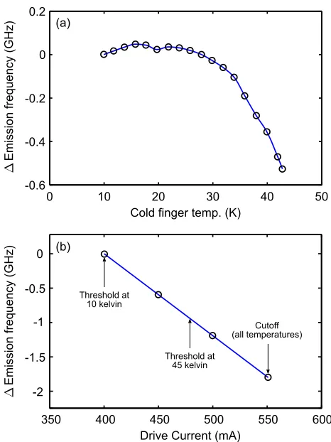
Fig. 3. Measured (a) thermal and (b) adiabatic modulation characteristics of the exemplar QCL. The data represent frequency offsets from the nominal 2.59 THz emission frequency due to cold finger temperature T0 and drive current I . These data, used to model frequency sweeping in our simulations, indicate that in principle the frequency modulation range can be almost doubled by combining the two mechanisms.

drive current I . The prediction of T is an essential part of the complete model as it determines thermal frequency modulation behavior as well as the laser’s internal operating state and values of its rate equation parameters.

dT(t) dt =

1 mcp(T)

I(t)V(T(t),I(t))−(T(t)−T0(t)) Rth(T)

(1)

C. Modeling Adiabatic and Thermal Modulation

Fig. 4. Modulation with 2μs, 485 mA drive pulses (color online). Rows show the response for three types of pulse, (a) positive-going current ramp of magnitude 40 mA atop the pulse, (b) no current ramp (i.e. a perfectly rectangular pulse) and (c) negative-going ramp of magnitude 40 mA atop the pulse. Parts (d), (e), and (f) are the lattice temperature transients responsible for thermal emission frequency change. Parts (g)(h)(i) show emission frequency change caused by the current ramp and temperature change together. Parts (j), (k), and (l) show the optical output for each pulse type, with black/broken lines as the reference condition (no optical feedback). Ripples in the solid line (red) are the LFI fringes resulting from optical feedback. Subtracting the reference trace from the LFI trace for each of these gives the SM signals shown in parts (m), (n), and (o). On the 2μs scale, very little frequency change is due to the thermal transient, as can be seen from (h), (k), and (n).

III. RESULTS ANDDISCUSSION

To demonstrate the effects of combining adiabatic and thermal modulation in a THz QCL, we modeled the exemplar device under optical feedback typical in LFI applications with three different pulse excitations, namely (a) a linearly increasing current ramp atop the pulse, (b) a rectangular pulse (i.e. no current change during the pulse), and (c) a linearly decreasing current ramp atop the pulse.

As both the current and thermal coefficients of emission frequency are negative for our exemplar device, we expect the two mechanisms to augment each other in (a) and counteract each other in (c). For pulse type (b), LFI fringes due only to temperature change would appear. For these simulations the external cavity length L was 2.272 m, the target reflectivity R=0.7, the re-injection efficiencyε=0.005 (giving Acket’s parameter [36] C = 1.93), and the cold finger temperature was set to T0 = 45 K in order to use the region where emission frequency is changing most rapidly with temperature [see Fig. 3(a)]. LFI signals in the laboratory are usually

acquired by direct measurement of the laser’s terminal voltage, but for convenience in these simulations we present them as optical output power.

A. Results for Pulsed Linear Frequency Sweep

Fig. 5. Pre-emphasis of a 20μs pulse to linearize frequency sweep, for evenly spaced and proportioned interferometric fringes. Red/broken lines are the results before pre-emphasis and blue/solid lines the results with pre-emphasis. Even small deviations from exact linearity [parts (a) and (c)] can cause significant irregularity in fringe spacing and proportions over the duration of the pulse (f). A spectral analysis of the SM signal [broken line in (e)] shows spectral spreading resulting from irregular fringe spacing [broken line in (f)], and restored fringe regularity via pre-emphasis evidenced by sharp spectral peaks [solid lines in (e) and (f)]. Harmonics seen in the solid line (e) are due to the non-sinusoidal nature of the LFI fringes.

The result for the flat-topped pulse, row (b), shows little frequency change (h) and consequently only one complete LFI fringe (n). This is due to no adiabatic frequency change (no change in current drive atop the pulse), and the timescale (2 μs) being much shorter than the thermal timescale. The one visible fringe is therefore due entirely to the thermal mechanism acting over the 2 μs pulse period.

With a positive-going adiabatic drive current (a), the much larger frequency change (g), due almost entirely to current drive, results in about nine fringes (m).

For the negative-going adiabatic drive (c), the emission frequency trend is reversed (i), with about seven fringes being produced (o). In (m), thermal augments adiabatic change, resulting in one additional fringe above the purely adiabatic fringe count. In (o), thermal counteracts adiabatic, resulting in one less fringe.

When the timescale of the pulses was extended to 20 μs, the frequency sweep was much greater as a result of a larger temperature change in the lattice, and more fringes appeared in parts (m) and (n). The spacing of fringes was however noticeably less consistent. With pulses of length 200 μs, additional fringes were present but fringe spacing was far less consistent, with most fringes grouped in the first third of the pulse where temperature change is most rapid. Such inconsistent fringe spacing and shape make extraction of target information challenging. Our proposed approach to mitigating this challenge is to apply a pre-emphasis component in drive current that exactly cancels the nonlinear component of the thermal sweep, thereby producing a linear frequency sweep and hence evenly spaced and proportioned LFI fringes.

B. Linearization of Frequency Sweep

The primary source of nonlinearity in swept frequency is the behavior of the thermal circuit, defined by Eq. (1), which determines lattice temperature. The lattice temperature cannot be quickly or directly controlled as it is a result

of temperature buildup due to self-heating produced by the drive current. Further, the rate of heat buildup in the lattice is governed by the thermal characteristics of the device, i.e. heat capacity and internal thermal resistance as well as that between the device and the heat sink. Thermal modulation therefore continues for some time after its original cause (current change) has ceased. The only means of control is via drive current, by introducing a pre-emphasis component that compensates for the thermally introduced nonlinearity. We achieved this by using the observed frequency sweep’s nonlinearity as the error term in a feedback control loop that modifies the drive current. Changing the drive current in turn alters self-heating, making the process require iteration until the required precision is reached. The drive current curve arrived at in this manner can then used to produce precisely linear emission frequency sweeps, provided no changes are made to operating conditions and parameters. Changes to cold finger temperature or the pulse amplitude limits and slope would, for example, require recalculation of the pre-emphasis drive current. The end result of the iterative process is a nonlinear current drive pulse that produces adiabatic and thermal frequency sweeps, both with nonlinear components that exactly cancel each other, to producing an overall linear frequency sweep.

To illustrate the linearizing process we use the drive pulse shown in Fig. 5 (a) (red/broken line). In this simulation a target reflectivity of R =0.03 (giving C =0.40) is used in order to reduce the harmonic content of the LFI signal. Before correcting the drive current, the maximum deviation from linearity of the frequency sweep [Fig. 5 (c)] is 52.6 MHz. The frequency sweep itself spans 868 MHz. After 5 iterations the maximum nonlinearity was reduced to 9.4 kHz, representing improvement by a factor of more than 103.

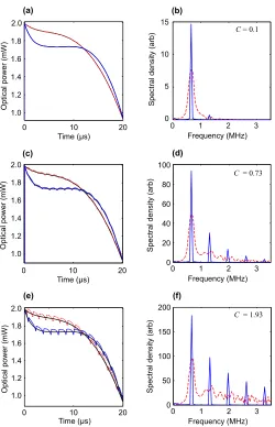
Fig. 6. Waveform (a), (c), and (e), and spectral content (b), (d), and (f), of SM signal for three values of Acket’s parameter, C =0.1 representing the very weak feedback regime, C = 0.73 representing the weak feedback regime, and C = 1.93, representing the moderate feedback regime. The spectra demonstrate that feedback in the very weak regime is required for low LFI signal harmonic content, i.e. near-sinusoidal fringes.

the frequency sweep. Part (a) shows the corrected current dipping below the linear ramp to compensate for the initially rapid frequency change at the start of the thermal transient. As the thermal transient settles, drive current increases more rapidly to compensate for the slower thermal frequency sweep near the end of the pulse, giving an overall linear frequency sweep [part (c)]. Although the uncorrected nonlinearity in frequency sweep appears to be slight, it has a marked effect on the interferogram [part (f)], with fringe width almost doubling over the duration of the pulse. After correction, the fringe proportions and spacing are constant over the duration of the pulse [part (f)]. Fast Fourier transforms of the SM sig-nals are shown in part (e) to demonstrate the efficacy of linearization resulting from the pre-emphasis: varying fringe spacing in the uncorrected sweep broadens the spectral peak, whereas the linearized sweep with perfectly spaced fringes result in sharp spectral peaks. Harmonics visible in the spec-trum are due to the non-sinusoidal nature of the SM signal. These can be somewhat mitigated with the use of less optical

feedback (lower values of C), but at a cost to signal-to-noise ratio (SNR). To illustrate how feedback strength (as encoded in Acket’s constant C) affects the harmonic content of the SM signal, we repeated the simulations for different values of C representative of three different feedback regimes [37], very weak (C = 0.1), weak (C = 0.73), and moderate (C = 1.93). The results are shown in Fig. 6. In the very weak feedback regime (C=0.1), the SM signal, barely visible in (a), is almost purely sinusoidal with second harmonic about 25 dB below the fundamental. However, the fundamental itself is about 15 dB below the fundamental in the weak feedback regime (C =0.73), resulting in a commensurately lower SNR. Correction of longer pulses, for example the pulse of Fig. 5 (a) time-scaled to a width 200μs, would require drive currents outside the laser’s operating region, and is therefore not possible. Shortening the pulse width on the other hand may compromise sweep range in applications being optimized for maximum frequency sweep. Frequency linearization in such applications is therefore limited to pulse widths of the order of the laser-submount thermal time constant. Since the time con-stant of the thermal circuit is fixed at manufacture and assem-bly time, tailoring the drive pulse width and swept frequency range to suit specifications or experimental requirements must be done at the design stage via modeling. Deliberately increas-ing the laser to submount thermal resistance, for example using an epoxy instead of indium interface, may educe the full potential of the thermal modulation characteristic of Fig. 3(a) at shorter pulse widths.

A similar approach to emission frequency linearization may be used to produce pulses that result in no frequency modulation, where modulation is undesirable. This can be achieved with a pulse shape for which the adiabatic and thermal modulation components exactly cancel each other.

IV. CONCLUSION

Using a realistic model of a QCL, we have demonstrated a method of swept-frequency LFI in pulsed-mode THz QCLs. We have shown that in addition to the known benefits of pulsing, namely higher optical output power and operating temperature, the shape of the drive pulse can be designed to increase and linearize the range of a QCL’s frequency sweep with a carefully considered combination of adiabatic and thermal modulation. This is of particular relevance in THz materials analysis where swept-frequency LFI is employed, but would also be important in any pulsed application affected by emission frequency change. We propose that this technique may be also useful in other laser applications that require a significantly extended and linear emission frequency sweep, such as trace gas detection, imaging, heterodyne mixing, and spectroscopy.

REFERENCES

[1] B. S. Williams, “Terahertz quantum-cascade lasers,” Nature Photon., vol. 1, no. 9, pp. 517–525, 2007.

[2] L. Li et al., “Terahertz quantum cascade lasers with >1 W output powers,” Electron. Lett., vol. 50, no. 4, pp. 309–311, Feb. 2014. [3] S. Fathololoumi et al., “Terahertz quantum cascade lasers operating up

pp. 396–404, Mar. 2010.

[9] C. A. Evans, V. D. Jovanovi´c, D. Indjin, Z. Ikoni´c, and P. Harrison, “Investigation of thermal effects in quantum-cascade lasers,”

IEEE J. Quantum Electron., vol. 42, no. 9, pp. 859–867, Sep. 2006.

[10] C. A. Evans et al., “Thermal modeling of terahertz quantum-cascade lasers: Comparison of optical waveguides,” IEEE J. Quantum Electron., vol. 44, no. 7, pp. 680–685, Jul. 2008.

[11] R. L. Tober, “Active region temperatures of quantum cascade lasers during pulsed excitation,” J. Appl. Phys., vol. 101, no. 4, p. 044507, 2007.

[12] M. S. Vitiello, G. Scamarcio, and V. Spagnolo, “Time-resolved mea-surement of the local lattice temperature in terahertz quantum cascade lasers,” Appl. Phys. Lett., vol. 92, no. 10, p. 101116, 2008.

[13] M. S. Vitiello and A. Tredicucci, “Tunable emission in THz quantum cascade lasers,” IEEE Trans. THz Sci. Technol., vol. 1, no. 1, pp. 76–84, Sep. 2011.

[14] S. Fathololoumi et al., “Thermal behavior investigation of terahertz quantum-cascade lasers,” IEEE J. Quantum Electron., vol. 44, no. 12, pp. 1139–1144, Dec. 2008.

[15] K. Pier´sci´nski et al., “Investigation of thermal properties of mid-infrared AlGaAs/GaAs quantum cascade lasers,” J. Appl. Phys., vol. 112, no. 4, p. 043112, 2012.

[16] G. Agnew et al., “Efficient prediction of terahertz quantum cascade laser dynamics from steady-state simulations,” Appl. Phys. Lett., vol. 106, no. 16, p. 161105, 2015.

[17] L. Jumpertz, S. Ferré, K. Schires, M. Carras, and F. Grillot, “Nonlinear dynamics of quantum cascade lasers with optical feedback,” Proc. SPIE, vol. 9370, p. 937014, Feb. 2015.

[18] Y. Petitjean, F. Destic, J.-C. Mollier, and C. Sirtori, “Dynamic modeling of terahertz quantum cascade lasers,” IEEE J. Sel. Topics Quantum

Electron., vol. 17, no. 1, pp. 22–29, Jan./Feb. 2011.

[19] A. Scheuring et al., “Transient analysis of THz-QCL pulses using NbN and YBCO superconducting detectors,” IEEE Trans. THz Sci. Technol., vol. 3, no. 2, pp. 172–179, Mar. 2013.

[20] R. Teysseyre, F. Bony, J. Perchoux, and T. Bosch, “Laser dynam-ics in sawtooth-like self-mixing signals,” Opt. Lett., vol. 37, no. 18, pp. 3771–3773, 2012.

[21] A. Valavanis et al., “Self-mixing interferometry with terahertz quantum cascade lasers,” IEEE Sensors J., vol. 13, no. 1, pp. 37–43, Jan. 2013. [22] R. Lang and K. Kobayashi, “External optical feedback effects on

semiconductor injection laser properties,” IEEE J. Quantum Electron., vol. QE-16, no. 3, pp. 347–355, Mar. 1980.

[23] T. Taimre, M. Nikoli´c, K. Bertling, Y. L. Lim, T. Bosch, and A. D. Raki´c, “Laser feedback interferometry: A tutorial on the self-mixing effect for coherent sensing,” Adv. Opt. Photon., vol. 7, no. 3, pp. 570–631, 2015. [24] Y. L. Lim et al., “Demonstration of a self-mixing displacement sensor based on terahertz quantum cascade lasers,” Appl. Phys. Lett., vol. 99, no. 8, p. 081108, 2011.

[25] G. Giuliani, M. Norgia, S. Donati, and T. Bosch, “Laser diode self-mixing technique for sensing applications,” J. Opt. A, Pure Appl. Opt., vol. 4, no. 6, pp. S283–S294, 2002.

[26] A. D. Raki´c et al., “Swept-frequency feedback interferometry using ter-ahertz frequency QCLs: A method for imaging and materials analysis,”

Opt. Exp., vol. 21, no. 19, pp. 22194–22205, 2013.

[27] S. S. Howard, Z. Liu, and C. F. Gmachl, “Thermal and stark-effect roll-over of quantum-cascade lasers,” IEEE J. Quantum Electron., vol. 44, no. 4, pp. 319–323, Apr. 2008.

[28] J. M. Hensley et al., “Spectral behavior of a terahertz quantum-cascade laser,” Opt. Exp., vol. 17, no. 22, pp. 20476–20483, 2009.

[29] A. Grier et al., “Origin of terminal voltage variations due to self-mixing in terahertz frequency quantum cascade lasers,” Opt. Exp., vol. 24, no. 19, pp. 21948–21956, 2016.

hertz quantum cascade lasers,” IEEE J. Sel. Topics Quantum Electron., vol. 23, no. 4, Jul./Aug. 2017, Art. no. 1200209.

[35] G. Agnew et al., “Model for a pulsed terahertz quantum cascade laser under optical feedback,” Opt. Exp., vol. 24, no. 18, pp. 20554–20570, 2016.

[36] G. Acket, D. Lenstra, A. D. Boef, and B. Verbeek, “The influence of feedback intensity on longitudinal mode properties and optical noise in index-guided semiconductor lasers,” IEEE J. Quantum Electron., vol. 20, no. 10, pp. 1163–1169, Oct. 1984.

[37] S. Donati and R.-H. Horng, “The diagram of feedback regimes revis-ited,” IEEE J. Sel. Topics Quantum Electron., vol. 19, no. 4, p. 1500309, Jul./Aug. 2012.

Gary Agnew (M’93) received the B.Sc. and M.Sc. degrees in electrical engineering from the University of the Witwatersrand, Johannesburg, South Africa, in 1985 and 1990, respectively. He is currently pursuing the Ph.D. degree with The University of Queensland, Australia. He has held various research positions in the instrumentation industry, focusing on microwave, photonic, and nucleonic sensor tech-nologies. His research interests include modeling terahertz quantum-cascade lasers.

Andrew Grier was born in Belfast, U.K. He received the B.Sc. degree (Hons.) in physics from the University of St Andrews, U.K., in 2009, and the M.Sc. and Ph.D. degrees in electronic and electrical engineering from the University of Leeds, U.K., in 2010 and 2015, respectively. He is currently a Senior Research and Development Engineer with Seagate Technology. His research interests include computational modeling of carrier transport in semiconductor quantum electronics and stochastic micromagnetic modeling of advanced magnetic recording devices.

Thomas Taimre received the B.Sc. degree in math-ematics and statistics, the B.Sc. degree (Hons. I) in statistics, and the Ph.D. degree in mathematics from The University of Queensland, Australia, in 2003, 2004, and 2009, respectively. He is currently a Lecturer of mathematics and statistics with The University of Queensland. He has co-authored the

Handbook of Monte Carlo Methods, which provides

Karl Bertling (S’06–M’12) received the B.E. degree in electrical engineering and the B.Sc. degree in physics, the M.Phil. degree in electrical engineering, and the Ph.D. degree in electrical engineering from The University of Queensland in 2003, 2006, and 2012, respectively. He has contributed to the body of knowledge for this technique, in visible, near-IR, mid-near-IR, and terahertz semiconductor lasers. His current research interests are imaging and sensing via laser feedback interferometry (utilising the self-mixing effect).

Yah Leng Lim received the B.Eng. and Ph.D. degrees in electrical engineering from The University of Queensland, Brisbane, Australia, in 2001 and 2011, respectively. From 2002 to 2005, he was a Research and Development Engi-neer with Philips Optical Storage, Singapore, focusing on the integration of optical and sensor technologies in optical storage systems. He currently holds the Advance Queensland Research Fellowship funded by the Queensland Government, focusing on the development of laser feedback interferometry imaging systems for the early detection of skin cancers.

Zoran Ikoni´c received the Ph.D. degree in elec-trical engineering from the University of Belgrade, Belgrade, Serbia, in 1987. During 1981–1999, he was with the Faculty of Electrical Engineering, Uni-versity of Belgrade. Since 1999, he has been with the School of Electronic and Electrical Engineer-ing, University of Leeds, Leeds, U.K. His current research interests include electronic structure and optical and transport properties of semiconductor nanostructures and devices.

Paul Dean received the M.Phys. degree (Hons.) in physics and the Ph.D. degree in laser physics from The University of Manchester, Manchester, U.K., in 2001 and 2005, respectively. In 2005, he joined the School of Electronic and Electrical Engineering, Institute of Microwaves and Photonics, University of Leeds, Leeds, U.K., as a Post-Doctoral Research Associate. His current research interests include ter-ahertz optoelectronics, quantum-cascade lasers, and terahertz imaging techniques. In 2011, he received a Fellowship from the Engineering and Physical Sciences Research Council, U.K.

Alexander Valavanis received the M.Eng. degree (Hons.) in electronic engineering from the University of York, York, U.K., in 2004, and the Ph.D. degree in electronic and electrical engineering from the University of Leeds, Leeds, U.K., in 2009. From 2004 to 2005, he was an Instrumentation Engineer with the STFC Daresbury Laboratory, Warrington, U.K. From 2009 to 2016, he was a Research Fellow with the University of Leeds. He is currently a Uni-versity Academic Fellow (tenure track) of terahertz instrumentation with the University of Leeds. His research interests include terahertz instrumentation, quantum-cascade lasers, silicon photonics, and computational methods for quantum electronics. He is a member of the Institution of Engineering and Technology.

Dragan Indjin received the B.S., M.S., and Ph.D. degrees in electrical engineering from the University of Belgrade, Serbia.

He joined the Faculty of Electrical Engineering, University of Belgrade, in 1989, where he later became an Associate Professor. Since 2001, he has been with the School of Electronic and Electrical Engineering, Institute of Microwaves and Photon-ics, University of Leeds, Leeds, U.K., where he is currently a Reader (Associate Professor) of opto-electronics and nanoscale opto-electronics. His research interests include the electronic structures, optical and transport properties, optimization and design of quantum wells, superlattices, quantum-cascade lasers, and quantum well infrared photodetectors from near- to far-infrared and terahertz spectral ranges. He is currently focused on applications of quantum-cascade lasers and interband cascade lasers for sensing and imaging applications.

Dr. Indjin was a recipient of the Prestigious Academic Fellowship from the School of Electronic and Electrical Engineering, Institute of Microwaves and Photonics, University of Leeds, in 2005. He is currently a Coordinator of major international projects on infrared and terahertz imaging and sensing for medical and security application.