Microcrack Parameters Characterization in Hard-Coatings Using Moments for Image Processing

Int. J. Electrochem. Sci., 8 (2013) 9677 - 9691

International Journal of

ELECTROCHEMICAL

SCIENCE

www.electrochemsci.org

Technical Report

Microcrack Parameters Characterization in Hard-Coatings

Using Moments for Image Processing

A. Femat-Diaz1,*, I. Terol-Villalobos2, J. Torres-Gonzalez2, F. Manríquez-Guerrero2, and D. Vargas-Vazquez1

1 _{Universidad Autónoma de Querétaro, Facultad de Ingeniería, División de Estudios de Posgrado.} Cerro de las Campanas s/n, Querétaro, Querétaro 76010, México.

2 _{Centro de Investigación y Desarrollo Tecnológico en Electroquímica S.C., Pedro Escobedo,} Querétaro 76700, México.

*

E-mail: [email protected]

Received: 18 October 2012 / Accepted: 18 March 2013 / Published: 1 July 2013

The purpose of this paper is to present an automatic, reliable technique to characterize length and orientation of microcracks in hard-coatings that is easy to implement. Consequently subjectivity due to human perception for measuring these characteristics of cracks can be eliminated. This study was done using optical microscope images of hard chromium coatings. For the measurements with image processing, geometric moments, which is a known technique, is useful. However, the segmentation of microcracks plays an important role in making these measurements. In this paper, four samples have been considered, and manual and automated measurements have been performed in order to note the similarities. The results of the automatic method are contrasted with the manual measurements for one image per sample. These results show there was not significant differences between methods. Next, the automatic measurements for groups of seventeen images per sample are compared to analyze differences between samples where there was evidence that a difference between samples existed. Confidence intervals for medians were calculated at 95% confidence. Significance for the differences in samples medians for cracks' length and angle were found to be p-value <0.001. Therefore, it was proven that the proposed technique is a very useful tool to characterize length and orientation in microcracks.

Keywords: crack characterization, hard coating, moments, orientation, major axis length

1. INTRODUCTION

properties. After fabrication, certain parts may contain surface defects such as scales, pits, mold marks, grinding lines, tool marks, or scratches.

Cracks in coating layers are caused by its re-crystallization process, that changes the structure from hexagonal face centered (hcp) to body centered cubic (bcc). It is known that bright electrodeposits are usually internally stressed, which is noticed in a high hardness. A tensile state of stress in the coating may cause the formation of cracks; chromium coatings have high tensile stress.

Residual stresses are inherent characteristics of electrolytic deposits; they depend on substrate metal, temperature, current density, and chemical concentrations of the electrolyte. Residual stresses can also be produced by plastic deformation heterogeneity during the process of electroplating [1]. They are classified as intrinsic or extrinsic [2]. The intrinsic stresses are developed in the deposit; while extrinsic ones are the result of the interaction of deposit and substrate [3].

It has been found that bright chromium coatings frequently begin to crack when the thickness is between 1 and 3 µm [4-6]. When a crack starts the local current density increases at its edges. Chromium is deposited faster at these edges which closes the crack. This phenomenon repeats in cycles as the deposit grows and closed cracks do not open again [4].

The prediction of structure problems allows the control of their degradation. Consequently, the detection and characterization of cracks on hard coatings is an important step in the fabrication of materials. The development of automated crack detection techniques and accurate methods for crack characterization are important for manufacturing applications.

In hard coatings the most important characteristics for micro-cracks are the length and their perpendicularity to the substrate. Some commercial packages have certain measurements that can be implemented in a semi-automatic or partially automatic way. However, the development of fully automated methods for the measurement of these characteristics is still under investigation.

Only one case where is used a technique to measure crack parameters with image processing was found. In 2005, Grande [7] reported a work where a Y projection to X projection ratio is used to measure vertical crack orientation, provided by Clemex Inc.Vision image analysis software. Also, it is well known in this field that determination of the degree to which a crack is perpendicular to the substrate should be included in the crack’s analysis.

For crack orientation, using all the points in the crack's shape is more robust than using only the two farthest points in a shape, as in Feret's diameters. A descriptor defined by all the pixels in a shape is less influenced by the presence or absence of a single pixel around the periphery [8]. The length of the crack is also an important parameter because longer cracks could produce fractures in coatings. Therefore, measurements of the maximum axis length and the angle with respect to the substrate become of great importance. Also, they can be obtained using all the points in a segment or crack using geometric moments. Further, statistical tools can be used to analyze the complete quantity of cracks in different samples of a material to compare their behavior.

2. MATERIALS AND METHODS

Chromium coatings were obtained from three aqueous solutions (a) Standard solution 250g/L CrO3 and 2.5 g/L H2SO4 as reference, (b) 250g/L CrO3 and 1.923 g/L H2SO4 and (c) 250g/L CrO3 and 3.125 g/L H2SO4. The samples were steel cylinders (3cm diameter x 8cm long).

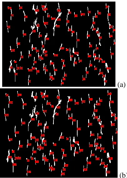
The electrodeposits were processed under different temperatures between 20 and 60°C and the current density variation was (20-60) A/dm2. The samples were rinsed and dried after plating. They were cut to obtain smaller samples, then polished and etched with the Murakami's acid (100 g/L K3 [Fe (CN6)], 8 g/L NaOH, water) to develop the micro-crack pattern and to be studied by using optic microscopy. A design of experiments utilizing 23 for coatings was used. The cracks in the samples SA, SB, SC, and SD, as are shown in Table 1, were characterized.

Table 1. Deposit conditions.

Sample Combination a b c a

[CrO3:H2SO4] b (°C)

c

(A/dm2)

-1 - - - B 20 20

a + - - C 20 20

SA b - + - B 60 20

SB ab + + - C 60 20

c - - + B 20 60

ac + - + C 20 60

SC bc - + + b 60 60

SD abc + + + c 60 60

For each one of the four samples, 17 microstructural images were acquired. They were captured with a Nikon epiphot 200 optical metallographic microscope which includes an integrated video system. The dimensions of the images were 640x480 pixels where 2.62 pixels represented 1µm.

The image processing consisted of two parts. The first phase was to segment the micro-cracks and the second was to measure the micro-cracks' parameters of interest. For the segmenting phase, let f be the original image and V_gray be the gray level that maximizes the variance between two groups of gray levels in f . The transformation gwas applied to improve the uniformity of these gray levels in the cracks.

( ) , if ( ) 0

( )

0 , otherwise

gray gray

f x V f x V

g x         

threshold value for imageg. This enabled investigators to separate cracks from the image background. Thus, the pixels are divided into two classes,

0 , if 0 g( ) ( ( ))

1 , if k+1 g( ) 1

x k T g x

x L

 



  _{  }



where kis the value of intensity that maximizes the variance between classes [9,10]. The image in Fig. 1 (c) is Otsu' result of the example, after which, a filter was required. In mathematical morphology, the basic filters are the morphological opening _B and the morphological closing _B with a given structuring element (SE). Brepresents the elementary SE (3x3 pixels, for example) containing its origin, and  is an homothetic parameter. Thus, the morphological opening and closing are given, respectively, by equations (1),

( ( )) ( ( ))

B B B f B B B f

     

      (1)

where the morphological erosion _B and dilation _Bare expressed as 1

( ) inf ( )

B f y B f x y

 

  _  and 1 ( ) sup ( )

B f y B f x y

 

  _  .

Other morphological filters are the opening and closing by reconstruction given as, 1 1 1

until stability

( ) lim nf( ( )) f... f f ( ( ))

n

f f f

  

      



 

1 1 1

until stability

( ) lim n_f( ( )) _f... _{f f} ( ( ))

n

f f f

  

      



  (2)

where 1_{f g( )}  f _B( )g with f g is the geodesic dilation of size one and 1

( ) ( )

f g f B g

   with f gis the geodesic erosion [9,11].

(a)

(b)

(c)

(e)

(f)

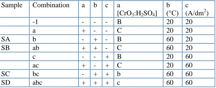
Figure 1. Operators sequence to segmentate mini-cracks in example image: (a) Original Image, (b) Subtracting max var, (c) Otsu umbralization, (d) Vertical closing, (e) Geodesic Opening, and (f) Without edge cracks.

For the measuring phase, inertia moments were used to evaluate the parameters for each crack. An inertia moment is a mathematical expression defined by the sum of the individual area elements multiplied by the square distance to its axis. It does not have physical meaning. A simple moment of order p q, is defined by equation (3), where f x y( , ) is the gray level in the x y, point in an image of

N M pixels. 1 1

,

0 0

( , ) M N

p q p q

x y

m x y f x y

 

 





For a segment determined by a region S, in a binary image, the moment is defined as

, ( , )

p q p q x y

m 



1 1 , 0 0 ( ) ( ) ( , ) M N p q p q x y

x x y y f x y

  

 





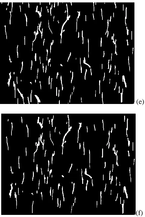
For each crack in an image the parameters indicated below were measured: 1. The angle θ to the ordinate axis, which represents the orientation, and 2. the major axis length.

The angle () of a segment defined in equation (5) is referred to as the minimum inertia axis. This is obtained through second order moments, defined either, ₂₀₀₂if it is to the abscissa axis, or

02 20

  if it is to ordinate axis. Therefore, a transformation θ was necessary to show the perpendicularity of the segment to the substrate. If the crack angle is measured anticlockwise a positive angle is obtained and if it is measured clockwise, a negative angle is obtained.

1,1 2,0 0,2 2 1 arctan 2       (5) 2,0 0,2 2,0 0,2

90, if and <0

90, if and 0

, otherwise

              _     

For moments, the maximum axis length Y_max of the segment in a binary image is defined in equation (6), with U_xx, U_yy, and U_xy as _2,0, _0,2, and _1,1 normalized, i.e.

2,0 0,0, 0,2 0,0, and 1,1 0,0

xx yy xy

U   U   U   respectively.

2 2

max 2 2 xx yy ( xx yy) 4 xy

Y  U U  U U  U (6)

(a)

(b)

Figure 2. Measuring results in example image: (a) Angles and (b) lengths.

A manual method was performed to have measurements to compare the ones obtained with the automatic method described above. This method was implemented as follow: Four images were selected, one per sample. The cracks for each image were measured visually identifying the two extreme points per crack ( ,x y_{1 1}) and ( ,x y_{2 2}) using software that allows showing the position and the color for the location of the cursor (the software used was Jack ® Paint Shop Pro). The cartesian coordinates for the points allowed to calculate the geometric distance and angle between them. The two extreme points for each crack ( ,x y_{1 1}) and ( ,x y_{2 2}) were used to estimated the crack length l as the geometric distance between these points, l



 



M

 in degrees was calculated as _M  arctan((x₂x ) (y_{1 2}y ))₁ .

Two statistical studies were carried out to assess the effectiveness of the proposed method, one to compare the results of the proposed automatic method against the manual method and the other to evaluate the differences between the samples.

3. RESULTS AND DISCUSSION

Total cracks per sample were 1500 for SA, 1862 for SB, 1305 for SC, and 1660 for SD. The area per image was 44752.64 μm2.

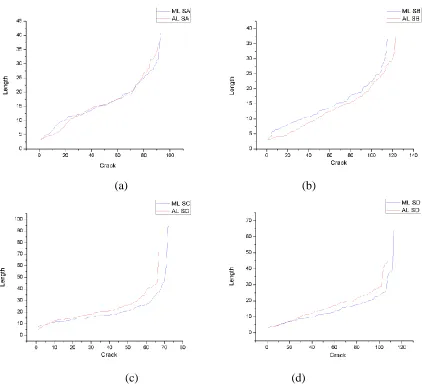
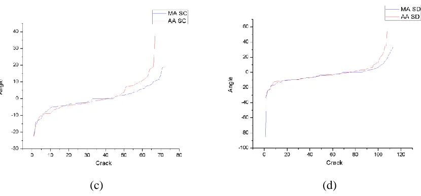
For the first comparison the images in Fig (3) were used as source and the results are presented in Fig (4) and Fig (5). These figures show the plots for the samples SA, SB, SC, and SD, where the horizontal axes are the cracks in ascending order according to the length and angle, respectively, and the vertical axes are the measurements (length and angle); the lines are red for the automatic measurements and blue for the manual measurements.

(a) (b)

(b) (d)

(a) (b)

(c) (d)

Figure 4. Length measurements for Sample A, B, C and, D. Manual against automatic method. (a) SA, (b) SB, (c) SC, (d) SD.

(c) (d)

Figure 5. Signed angle measurements for Sample A, B, C and, D. Manual against automatic method. (a) SA, (b) SB, (c) SC, (d) SD.

The results of statistical analysis have shown that the distributions of the length and angle, for both methods (manual and automatic) were not normal. Thus, a Kruskal-Wallis non parametric test, which does not assume a normal distribution, was used for examine the data. The p-values are presented in the Table (2) considering α=.05. These results indicate there are no significant differences between methods, because all are greater than α.

Table 2. p-values to compare manual against automatic method. Sample Length Angle SA 0.73762 0.16036 SB 0.19587 0.57124 SC 0.1971 0.56019 SD 0.09063 0.75857

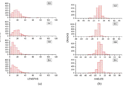
(a) (b)

Figure 6. Measuring results for the automatic method. Four samples with seventeen images per sample. (a) Angles and (b) lengths.

Table 3. Confidence intervals for samples.

Sample Median Length StdDev Length Median Angle StdDev Angle SA 11.694 - 13.044 9.120 - 9.797 -3.1402 -

2.1509

13.8729 - 14.9028 SB 10.274 - 11.336 7.876 - 8.399 2.5070

-1.3471

13.8460 - 14.7651 SC 17.432 - 18.693 10.995 - 11.872 0.7407 -

0.1368

10.6052 - 11.4517 SD 16.241 - 17.430 9.838 - 10.531 1.0291

-0.1153

11.8642 - 12.7000 Mood's

Test p-value

< 0.001 < 0.001 < 0.001 < 0.001

while the automatic method considers all points of the shape. The orientation results are more similar between manual and automatic method.

For the comparative analysis between samples the data obtained with the 17 images per sample were used with the automatic method. The results for length and angle are shown in the histograms in Fig. (6) (a) and (b) respectively. With them a general tendency of the measured parameters for the samples can be analyzed. The histograms and confidence intervals of Table (3) provide information to analyze differences between the samples.

For the statistical analysis that compares the treatments, the length and the angle were the variables used as reponses. SA, SB, SC, and SD were the four factors whose medians were compared statiscally as follow H₀:xSAxSB xSC xSD for the length and the angle. The medians were compared with a Mood’s Test, which is a nonparametric test, to assess such null hypothesis for the four samples in this case. The result of the test was p-value <0.001, meaning that medians for the samples are actually different, or that the null hypothesis was false; hence the samples were found statistically distinct. Therefore, there is evidence that a difference between samples exists [13]. Confidence intervals for medians were calculated at 95% confidence. The intervals showed differences in the cracks' lengths and angles per sample (see Table 3). Angles are not as well differentiated as lengths; however, the tests demonstrated clear evidence of their differences.

The Table (3) shows the confidence intervals for angles and lengths of the cracks, the samples can be differentiated based on these intervals and the sample SC has the longest cracks with the largest angles, its intervals were 17.432 – 18.693 for the median length and 0.7407 – 0.1368 for the median angle. This sample was found to present the largest effect out of the four.

The sample SB shows the shortest cracks with median in the interval of 10.274 – 11.336, however its angles were not the smallest but they were only average with median between -2.5070 – 1.3471. The sample SD shows the second longest cracks with median from 16.241 – 17.430 and the smallest angles of all the samples with median between -1.0291 – 0.1153. The sample SA shows the largest angles from -3.1402 – 2.1509 in median, but its cracks were the second smallest with median 11.694 – 13.044.

The results in Table (3) show relevant characteristics of micro-cracks in hard-coatings. By comparing the deposit conditions illustrated in Table (1), it is possible to identify the effect of the current density. That is, at low current density the effect “chicken wire” may occur [14], and in this case, the micro-cracks have small sizes and their orientations, regarding deposit orientation, also tend to disperse. Similarly, having high current densities, the size of the cracks increases and maintains a good directionality [15, 16].

4. CONCLUSIONS

These methods are rough approximations of crack characterizations. In this investigation, an automatic method was developed and compared with a manual characterization of length and orientation of cracks; in contrast to the manual measurements that are limited to the visual accuracy and training of those who make the measurements. The proposed automatic method takes into account the whole set of points that make up the shape of the crack, so that it does not depend on external factors. This method is closer to the actual assessment of the defects in the material, which facilitates its characterization.

Comparisons are made between the methods and find that the length of the cracks using the automatic method is slightly larger. For the orientation angle the differences are smaller. The automatic method calculates the orientation based on all points in the crack while the manual method only considers two points.

The image processing methodology and the data analysis provide an accurate and automated process for cracks characterization based on two of the key variables for cracks' physical analysis. The methodology proposed, including the image processing method and the statistical analysis provides a good characterization of the cracks patterns in metal coatings. It allows better understanding of the cracks beyond the simple cracks density, adding information regarding length and angle against substrate.

ACKNOWLEDGMENTS

The authors thank the government agency CONACyT for the financial support. This work was funded by the project (133697) and the "Fondo Sectorial de Investigación para la Educación" (SEP-CONACyT 2007 - México). The authors would also thank Silvia C. Stroet for her assistance in editing the English content of this paper.

References

1. M. Aroyo, D. Stoychev and N. Tzonev, Plat. Surf. Finish., 85 (1998) 92.

2. N.M. Martyak, J.E. McCaskie, B. Voss and W. Plieth, J Mat Sci, 32 (1997) 6069. 3. R. Weil, Plating, 57 (1970) 1231.

4. A.R. Jones, Corrosion of electroplated hard chromium, ASM Handbook Corrosion, ASM

International, Member/Customer Service Center, Materials Park, OH 44073-0002, USA, 13 (1987). 5. C. P. Britain and G.C. Smith, Trans. Inst. Met. Finish., 33 (1956) 289.

6. H. Fry, Trans. Inst. Met. Finish., 32 (1955) 107. 7. J. Grande, Microsc. Microanal., 11 (2005) 1758.

8. J.C. Russ, The Image Processing Handbook, CRC Press, Boca Ratón, FL, USA, (2007).

9. P. Soille, Morphological Image Analysis, Principles and Applications 2nd ed., Springer-Verlag, Berlin, Heidelberg, New York, (2002).

10.B. Jähne, Digital Image Processing, Springer-Verlag, Berlin, Heidelberg, (2005).

11.L.A. Morales-Hernandez, I.R. Terol-Villalobos, A. Dominguez-Gonzalez, F. Manriquez-Guerrero and Herrera-Ruiz, G., J. Mater. Process. Technol., 210 (2010) 335.

12.R. Gonzalez and R. Woods, Digital Image Processing, Pearson Education-Prentice Hall, Upper Saddle River, NJ, (2008).

14.Grace F. Hsu, SAE Technical Paper 880863 (1988).

15.J. Torres-González, F. Castaneda and P. Benaben, Theoretical and Experimental Advances in Electrodeposition, ISBN: 978-81-308-0224-4, 101 (2008).

16.P. Benaben, F. Castañeda, R. Antaño, J. Morales, I. Terol and J. Torres-González, Superficies y Vacío, 25 (2012) 106.