Evolving Graphs by Graph Programming

This is a repository copy of

Evolving Graphs by Graph Programming

.

White Rose Research Online URL for this paper:

http://eprints.whiterose.ac.uk/126500/

Version: Accepted Version

Proceedings Paper:

Atkinson, Timothy, Plump, Detlef orcid.org/0000-0002-1148-822X and Stepney, Susan

orcid.org/0000-0003-3146-5401 (2018) Evolving Graphs by Graph Programming. In:

Proceedings 21st European Conference on Genetic Programming (EuroGP 2018). Lecture

Notes in Computer Science . Springer .

https://doi.org/10.1007/978-3-319-77553-1_3

eprints@whiterose.ac.uk https://eprints.whiterose.ac.uk/

Reuse

Items deposited in White Rose Research Online are protected by copyright, with all rights reserved unless indicated otherwise. They may be downloaded and/or printed for private study, or other acts as permitted by national copyright laws. The publisher or other rights holders may allow further reproduction and re-use of the full text version. This is indicated by the licence information on the White Rose Research Online record for the item.

Takedown

If you consider content in White Rose Research Online to be in breach of UK law, please notify us by

Evolving Graphs by Graph Programming

Timothy Atkinson⋆_{, Detlef Plump, and Susan Stepney}

Department of Computer Science, University of York, UK

{tja511,detlef.plump,susan.stepney}@york.ac.uk

Abstract. Rule-based graph programming is a deep and rich topic. We present an approach to exploiting the power of graph programming as a representation and as an execution medium in an evolutionary algorithm (EGGP). We demonstrate this power in comparison with Cartesian Ge-netic Programming (CGP), showing that it is significantly more efficient in terms of fitness evaluations on some classic benchmark problems. We hypothesise that this is due to its ability to exploit the full graph struc-ture, leading to a richer mutation set, and outline future work to test this hypothesis, and to exploit further the power of graph programming within an EA.

1

Introduction

Representation is crucial in computer science, and an important specific rep-resentation is the graph. Graphs are used in a wide range of applications and algorithms, see for example [4, 22, 5]. In evolutionary algorithms (EAs), graphs are used in some applications, but are usually encoded in a linear genome, with the genome undergoing mutation and crossover, and a later “genotype to phe-notype mapping” used to decode the linear genome into a graph structure. For example in Cartesian Genetic Programming (CGP) [14, 12], the connections of feed forward networks are encoded in a linear genome. NEAT [24, 23] provides a linear encoding of ANNs which are seen as graph structures. Trees (a subset of more general graphs) are also used in EAs. Grammatical Evolution [15, 21] uses a linear genome of integers to indirectly encode programs. Genetic Programming [7, 6] is unusual for an EA: rather than using a linear genome, it typically directly manipulates abstract syntax trees. Poli [20, 19] uses a ‘graph on a grid’ repre-sentation: the underlying structure is a graph, but the nodes are constrained to lie on discrete grid points. MOIST [8] proposes using trees with multiple output nodes and sharing to extend traditional genetic programming to domains where problems have multiple, related outputs. Pereira et al [16] represent Turing ma-chines as graphs encoded in a linear genome, and develop a crossover operator based on the structure of the underlying graph.

There are arguments for and against linear genomes representing graphs. Linear genomes are standard in EAs, and they can exploit the knowledge about

⋆_{Supported by a Doctoral Training Grant from the Engineering and Physical Sciences}

evolutionary operators. However, they can hide the underlying structure of the problem, and can have biases in the effect of the evolutionary operators. There may be advantages in evolving graphs directly, rather than via linear genome encodings or 2D grid encodings, and defining mutation operators that respect the graph structure. Direct graph transformation has deep theoretical under-pinnings, and has become increasingly accessible through efficient graph pro-gramming languages such as GP 2 [17, 2]. GP 2 enables high-level problem solv-ing in the domain of graphs, freesolv-ing programmers from handlsolv-ing low-level data structures. It has a simple syntax whose basic computational units are graph transformation rules which can be graphically edited. Also, GP 2 comes with a concise operational semantics to facilitate formal reasoning on programs.

Here we exploit an extension to GP 2 [1] that has probabilistic elements to support EA applications. We perform experiments of evolving graphs directly, and compare the results with experiments previously done with CGP. Using graph transformations, we write evolutionary operators as graph transformation rules, and we calculate fitness in the same context. Our results indicate that direct evolution can be significantly more efficient (significantly fewer fitness function evaluations) than basic CGP, due to the increased number of mutations available, allowing more effective exploration of the search landscape.

The paper is organised as follows. In§2 we overview Graph Programming. In §3 we describe how we have incorporated an EA into graph programming (EGGP). In §4 we compare our EGGP setup with Cartesian Genetic Program-ming (CGP). In§5 we describe benchmark experiments, and in §6 provide the results, demonstrating that EGGP is significantly more efficient, in terms of fit-ness evaluations, than vanilla CGP. In§7 we draw conclusions and outline future work in examining the reasons for this improvement.

2

Graph Programming

This section is a (very) brief introduction to the graph programming language GP 2; see [18] for a detailed account of the syntax and semantics of the language. A graph program consists of declarations of graph transformation rules and a main command sequence controlling the application of the rules. Graphs are directed and may contain loops and parallel edges. The rules operate on host graphs whose nodes and edges are labelled with integers, character strings or lists of integers and strings. Variables in rules are of type int, char, string,

Main:=link!

link(a,b,c,d,e:list)

a

1

c

2

e

3

b d a

1

c

2

e

3

b d

where not edge(1,3)

Fig. 1: A GP 2 program computing the transitive closure of a graph.

The principal programming constructs in GP 2 are conditional graph-trans-formation rules labelled with expressions. The program in Figure 1 applies the single rulelinkas long as possible to a host graph. In general, any subprogram can be iterated with the postfix operator “!”. Applying link amounts to non-deterministically selecting a subgraph of the host graph that matches link’s left graph, and adding to it an edge from node 1 to node 3 provided there is no such edge (with any label). The application conditionwhere not edge(1,3)

ensures that the program terminates and extends the host graph with a minimal number of edges. Rule matching is injective and involves instantiating variables with concrete values. We remark that GP 2’s inherent non-determinism is useful as many graph problems are naturally multi-valued, for example the computation of a shortest path or a minimum spanning tree.

Given any graphG, the program in Figure 1 produces the smallest transitive graph that results from adding unlabelled edges to G. (A graph is transitive

if for each directed path from a node v1 to another nodev2, there is an edge

from v1 to v2.) In general, the execution of a program on a host graph may

result in different graphs, fail, or diverge. The semanticsof a program P maps each host graph to the set of all possible outcomes [17]. GP 2 is computationally complete in that every computable function on graphs can be programmed [18]. Commands not used in this paper are the non-deterministic application of a set of rules and various branching commands.

While rule matching in GP 2 is non-deterministic, the refined language P-GP 2 (forProbabilistic GP 2) selects a match for a rule uniformly at random [1]. This language has been used to obtain the results described in the rest of this paper.

3

Evolving Graphs by Graph Programming (EGGP)

3.1 Representation

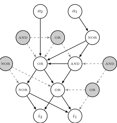
Our approach uses the following representation of individual solutions. An indi-vidualIover function setF ={f1, f2, ...fn} is a directed graph containing a set

i2 i1

NOR OR OR

NOR OR AND AND

AND OR NOR

o2 o1

Fig. 2: An example EGGP Individual for a binary logic problem.

that all functions in F (and the fitness function) operate on a single domain. EGGP individuals are defined in Definition 1.

Further, for each function nodev labelled with a functionf of arityn,vhas outgoing edges e1, ..., e_n such that for i = 1, ..., n, a(ei) = i. Then a provides

the order in which to passv’s inputs to f, resolving ambiguity for asymmetric functions. We assume acyclic graphs in this work, and hence an individual I

represents a solution as a network, where each node computes a function on its inputs (which are given by its outgoing edges). We refer to acyclic EGGP individuals as being “feed-forward”.

Definition 1 (EGGP Individual). An EGGP Individual over function setF is a directed graph I = {V, E, s, t, l, a, Vi, Vo} where V is a finite set of nodes

and E is a finite set of edges. s: E → V is a function associating each edge with its source. t:E → V is a function associating each edge with its target. Vi ⊆ V is a set of input nodes. Each node in Vi has no outgoing edges and is

not associated with a function.Vo⊆V is a set of output nodes. Each node inVo

has one outgoing edge, no incoming edges and is not associated with a function. l:V →F labels every “function node” that is not in Vi∪Vo with a function in

F.a:E→Zlabels every edge with a positive integer.

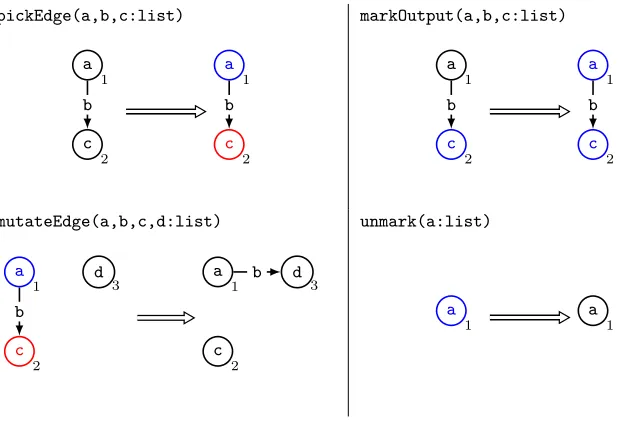
Main:=pickEdge;markOutput!;mutateEdge;unmark! pickEdge(a,b,c:list) a 1 c 2 b a 1 c 2 b markOutput(a,b,c:list) a 1 c 2 b a 1 c 2 b mutateEdge(a,b,c,d:list) a 1 c 2 d 3 b a 1 c 2 d 3 b unmark(a:list) a 1 a 1

Fig. 3: Mutating an edge of an EGGP individual while preserving feed-forwardness using a graph program.

output nodes, labeledo1ando2. Neutral material, which does not contribute to

the phenotype of the individual, is coloured gray. Edge labels are omitted for visual clarity, and is unambiguous for this example as all of the functions in F are symmetrical.

3.2 Atomic Mutations

We describe two point mutations for an EGGP individual that appear maximally simplistic; changing the function associated with a node and changing a single input to a node.

As we assume that individuals are feed-forward in this work we require a mutation that respects this constraint. A point mutation of a node’s input edge while maintaining feed-forwardness is shown in Figure 3. Firstly an edge to mutate is chosen and marked, with uniform probability, withpickEdgeand then all nodes which have a path to the source of the chosen edge are marked using

mutateFunction-fy(fx:string)

fx

1

fy

1

Fig. 4: Mutating the function of an EGGP individual’s node to some function

fy.fxis the existing function of the node being mutated, and an equivalent rule can be constructed for each function in the function set.

applying any restraints to the individual or the mutation, by transforming the individual using a graph program.

A point mutation of a node’s function is shown in Figure 4. Here node 1 has its function updated to some function fy ∈ F. This operator clearly pre-serves feed-forwardness as it introduces no new edges. In this work we deal with function sets with fixed, common arities. However, this may not always be de-sirable, for example when attempting symbolic regression over a function set containing both addition and sin operators. In the C-based library for Cartesian Genetic Programming this is overcome by simply using the first few inputs for lower arity functions [26], but in EGGP this would prevent some feed-forward preserving mutations when a node appears to contribute to the input of another but in truth does not. Although we do not address this issue in this work, we propose that it would be possible to add and delete input edges when mutating a node’s function to maintain correct function arities, while also maintaining feed-forwardness when adding those new input edges in a similar manner to the algorithm for edge mutations given in Figure 3.

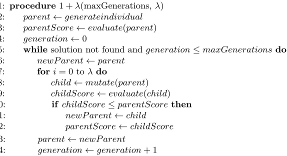
3.3 Evolutionary Algorithm

1: procedure1 +λ(maxGenerations,λ) 2: parent←generateindividual 3: parentScore←evaluate(parent) 4: generation←0

5: whilesolution not found andgeneration≤maxGenerationsdo 6: newP arent←parent

7: fori= 0 toλdo

8: child←mutate(parent) 9: childScore←evaluate(child) 10: if childScore≤parentScorethen 11: newP arent←child

12: parentScore←childScore 13: parent←newP arent

14: generation←generation+ 1

Fig. 5: The 1 +λevolutionary algorithm with neutral drift enabled.

3.4 Parameters

Use of the EGGP representation and the 1 +λ algorithm is parameterised by the following items:

• mr: the mutation rate. Nodes and edges have no particular order in EGGP, and the order in which feed-forward edges are mutated may influence the availability of future mutations. We therefore opt to generate the number of node mutations and edge mutations to apply to the individual using binomial distributions (simulating one probabilistic mutation for each node or edge) and then distribute these mutations across the individual at random.

• λ: the number of individuals to generate in each generation of the 1 +λ

algorithm.

• F: A function set. The maximum arity of functions inF is used to specify the number of input edges associated with each function node.

• n: the number of function nodes to use in each individual.

• p: the number of inputs that each individual should have to interface with the fitness function (|Vi|=p).

• q: the number of outputs that each individual should have to interface with the fitness function (|Vo|=q).

• A fitness function used to evaluate each individual.

4

Relation to Cartesian Genetic Programming

4.1 Cartesian Genetic Programming

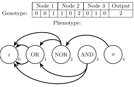
Node 1 Node 2 Node 3 Output Genotype: 0 0 1 1 0 2 0 1 0 2

Phenotype:

i

0 OR 1 NOR 2 AND 3

o

4

Fig. 6: The genotype-phenotype mapping of a simple CGP individual consisting of 1 input, 3 nodes and 1 output and arity 2. Each node is represented by 3 genes; the first 2 describe the indices of the node’s inputs (starting at index 0 for the individual’s inputi) and the third describing the node’s function. Function indices 0, 1 and 2 correspond to AND, OR and NOR respectively. The final gene describes the index of the node used by the individual’s output o. .

that all input connections must respect that ordering, preventing cycles. When evolving over a function set where each function takes 2 inputs, there are 3 genes for each node in the individual; 2 representing each of the node’s inputs, and 1 representing the node’s function. Outputs are represented as single genes describing the node in the individual which corresponds to that output. These connection genes (nodes’ input genes and the singular output genes) point to other nodes based on their index in the ordering.

An example genotype-phenotype mapping is given in Figure 6. Here an indi-vidual consisting of 3 nodes over a function set of arity 2, 1 input and 1 output is represented by 10 genes. These genes decode into the shown directed acyclic graph. In CGP individuals may be seen as a grid ofnr rows andnc columns; a node in a certain column may use any node from any row in an earlier column as an input. Hence the totaln=nr×nc nodes are ordered under a≤operator. The example shown in Figure 6 is a single row instance of CGP.

4.2 Comparison to EGGP

Here we demonstrate that EGGP provides a richer representation than CGP:

• For a fixed number of nodesnand function setF, any CGP individual can be represented as an EGGP individual, whereas the converse may not always hold when the number of rows in a CGP individual is greater than one.

i

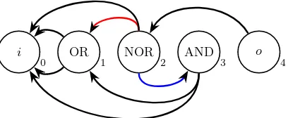
0 OR 1 NOR 2 AND 3

o

4

Fig. 7: A feed-forward preserving edge mutation. An edge (red) directed from node 2 to node 1 is replaced with an edge (blue) directed to node 3. This mutation produces a valid circuit but is impossible in CGP as it does not preserve order.

Firstly, consider the genotype-phenotype decoding of a CGP individual. Here we have clearly defined sets of input, output and function nodes. Additionally each function node is associated with some function from the function set, and there are ordered input connections (edges) from each function node to its inputs. Clearly this decoded individual can be treated as an EGGP individual fitting Definition 1. Conversely, consider the case wherenr>1. Then there is the trivial counter example of an EGGP individual with a solution depth greater than nc (as n > nc) which clearly cannot be expressed as a CGP individual limited to depthnc.

We now consider mutations available over a CGP individual in comparison to those for an EGGP individual where feed-forward preserving mutations are used. Clearly, as each order preserving mutation is feed-forward preserving, any valid mutation for the CGP individual is available for its EGGP equivalent. However, consider the example shown in Figure 7. Here a feed-forward mutation, connecting node 3 to node 4 is available in the EGGP setting but is not order preserving so is impossible in the CGP setting. Additionally, the semantic change that has occurred here, where an active node has been inserted between two adjacent active nodes is a type of phenotype growth that is impossible in CGP. Hence every mutation available in CGP is available in EGGP for an equivalent individual but the converse may not be true.

Therefore the landscape described by EGGP over the same function set and number of nodes is a generalisation of that described by CGP, with all individual solutions and viable mutations available, alongside further individual solutions and mutations that were previously unavailable.

4.3 Ordered EGGP (O-EGGP)

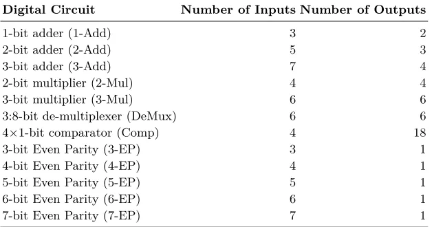
Digital Circuit Number of Inputs Number of Outputs

1-bit adder (1-Add) 3 2

2-bit adder (2-Add) 5 3

3-bit adder (3-Add) 7 4

2-bit multiplier (2-Mul) 4 4

3-bit multiplier (3-Mul) 6 6

3:8-bit de-multiplexer (DeMux) 6 6 4×1-bit comparator (Comp) 4 18

3-bit Even Parity (3-EP) 3 1

4-bit Even Parity (4-EP) 4 1

5-bit Even Parity (5-EP) 5 1

6-bit Even Parity (6-EP) 6 1

7-bit Even Parity (7-EP) 7 1

Table 1: Digital Circuit benchmark problems.

than order-preserving, input mutations, we compare performance against an ordered variant of EGGP, called Ordered EGGP.

Each node in an O-EGGP individual is associated with an order in an analo-gous manner to CGP. Node function mutations from EGGP are used, but input mutations are order-preserving rather than feed-forward preserving. Hence the same set of mutation operators, with the same probability distribution over their outcomes, is available for equivalent O-EGGP and CGP individuals. This approach simulates the landscape and search process of CGP under identical conditions, so should produce identical results to an equivalent CGP implemen-tation. By also benchmarking O-EGGP we demonstrate that it is EGGP’s free graphical representation and the associated more general ability to mutate in-put connections with respect to preserving feed-forwardness that yields higher quality results.

5

Benchmarking

a candidate solution in comparison to the full truth table of the given problem as the fitness function.

Each algorithm is run 100 times, with a maximum generation cap of 20,000,000; every run in each case successfully produced a result with the exception of the 3-Mul for CGP, which produced a correct solution in 99% of cases. In all 3 bench-marks, 100 nodes are used for each individual. Following conventional wisdom for CGP, we use a mutation rate of 4% for CGP and O-EGGP benchmarks. Ad-ditionally, a single row of nodes is used in each of these cases (nr= 1). However, from our observations EGGP works better with a lower mutation rate, so for EGGP benchmarks we use 1%. An investigation of how mutation rate influences the performance in EGGP is left for future work. The 1 +λalgorithm is used in all 3 cases, withλ= 4. Due to time constraints, O-EGGP is only benchmarked on easier problems; 1-Add, 2-Add, 2-Mul, DeMux, 3-EP, 4-EP and 5-EP. We argue that if the results from these benchmarks are in line with the CGP bench-mark results we may extrapolate that O-EGGP is indeed simulating CGP. In this case the two distinguishing factors between the EGGP and CGP benchmarks are the use of mutation operator (feed-forward preserving vs. order preserving) and mutation rate (1% vs. 4%).

To provide comparisons, we use the following metrics; median number of evaluations (ME), median absolute deviation (MAD; median of the absolute de-viation from the evaluation median ME), and interquartile range (IQR). The number of evaluations taken for each run is calculated as the number of gener-ations used multiplied by the total population size (1 +λ= 5). The hypotheses we investigate for these benchmarks are:

1. EGGP performs significantly better than CGP on the same problems under similar conditions. This hypothesis, if validated, would demonstrate the value of our approach.

2. O-EGGP does not perform significantly better or worse than CGP on the same problems under identical conditions. This hypothesis, if validated, would indicate that the possible factors influencing EGGP’s greater perfor-mance for the first hypothesis would be reduced to the use of the feed-forward mutation operator and the mutation rate.

6

Results

Here we present results from our benchmarking experiments. Digital circuit re-sults for EGGP and CGP are given in Table 2; rere-sults for O-EGGP on a smaller benchmark suite are given in Table 3.

To test for statistical significance we use the two-tailed Mann-Whitney U

EGGP CGP

Problem ME MAD IQR ME MAD IQR p A

1-Add 5,723 3,020 7,123 6,018 3,312 7,768 0.62 – 2-Add 74,633 32,863 66,018 180,760 88,558 198,595 10−15 _0.82

3-Add 275,180 114,838 298,250 2,161,378 957,035 1,837,942 10−31 _0.97

2-Mul 14,118 5,553 12,955 10,178 5,258 14,459 0.018 0.60 3-Mul 1,241,880 437,210 829,223 15,816,940 7,948,870 19,987,744 10−34 _0.99

DeMux 16,763 4,710 9,210 20,890 6,845 14,063 0.013 0.60 Comp 262,660 84,248 174,185 1,148,823 425,758 1,012,149 10−31 _0.97

3-EP 2,755 1,558 4,836 4,365 2,530 5,345 0.038 0.58 4-EP 13,920 5,803 11,629 22,690 11,835 24,340 10−6 _0.69

5-EP 34,368 15,190 30,054 106,735 55,615 126,063 10−18 _0.86

6-EP 83,053 33,273 66,611 485,920 248,150 535,793 10−3 _0.97

7-EP 197,575 61,405 131,215 1,828,495 843,655 1,860,773 10−33 _0.99

Table 2: Results from Digital Circuit benchmarks for CGP and EGGP. The p

value is from the two-tailed Mann-WhitneyU test. Wherep < 0.05, the effect size from the Vargha-Delaney A test is shown; large effect sizes (A >0.71) are shown in bold. The values for CGP on the 3-Mul problem include the single failed run.

Comparing EGGP to CGP in Table 2, we find no significant improvement of EGGP over CGP for small problems (1-Add, 2-Mul). Indeed, for 2-Mul CGP significantly outperforms EGGP (p <0.05), albeit with a small effect size (0.56<

A < 0.64). As the problems get larger and harder we find significant (p <

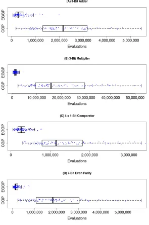
0.05) improvement of EGGP over CGP in all cases. The effect size is small (0.56<A<0.64) for the 3:8-Bit De-Mux and 3-Bit Even Parity, and medium (0.64<A<0.71) for 4-EP. We find highly significant (p <0.001) improvements along with large effect sizes (0.71<A) on all other problems, including the most difficult problems: 3-Add, 3-Mul, 4×1-Bit Comparator and 7-Bit Even Parity. So there is a clear progression of increasing improvement with problem difficulty. We visualise some highly significant results as box-plots, with raw data over-layed and jittered, in Figure 8. For each of the named problems, it can be clearly seen that EGGP’s interquartile range shares no overlap with CGP’s, highlight-ing the significance of the improvement made. Overall, we see these results to validate our first hypothesis that EGGP performs significantly better than CGP when addressing the same harder problems, although we note that no significant improvement is made for simpler problems.

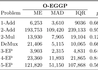
O-EGGP

Problem ME MAD IQR p

1-Add 6,253 3,610 9036 0.66 2-Add 193,753 109,420 239,133 0.95 2-Mul 13,930 7,905 19,104 0.12 DeMux 21,406 5,115 10,065 0.66 3-EP 3,903 2,315 4,831 0.64 4-EP 23,360 11,893 21,865 0.84 5-EP 121,820 51,150 107,868 0.56

Table 3: Results from Digital Circuit benchmarks for O-EGGP on a smaller benchmark suite. Thepvalue is from the two-tailed Mann-Whitney significance test comparing against CGP; no result is statistically significant (α= 0.05).

We believe that these findings support our hypothesis that O-EGGP does not perform significantly better or worse than CGP on identical problems under iden-tical conditions. As O-EGGP theoreiden-tically simulates CGP, this indicates that we can consider the differences between the runs of EGGP and O-EGGP, namely feed-forward preserving mutations and mutation rate, as the major contributors to the differences in performance shown in Table 2.

Further, we suggest that the significant differences in results would not be resolved by tuning the mutation rate parameter. Therefore we turn our atten-tion to the feed-forward preserving input mutaatten-tion operator. As shown in Fig-ure 7, feed-forward preserving mutations may insert nodes between nodes that would be considered adjacent in the CGP framework. This allows a subgraph of the solution to grow and change in previously unavailable manners. Performing functionally equivalent mutations with order preserving input mutations might require the construction of an entirely new subgraph in the neutral component of the individual which is then activated. We propose that the former mutation is more likely to occur than the sequence of mutations required to achieve the latter. Therefore where those unavailable mutations are “good” mutations in the sense of the fitness function, better performance will be achieved by using them directly. A future investigation into the quality of the neighborhood when using the feed-forward preserving mutation would clarify this hypothesis.

are also possible, freeing up genetic material to be used elsewhere. How useful these neutral mutations in the active component are is left for future work.

7

Conclusion and Future Work

We have proposed graphs as a fundamental representation for evolutionary algo-rithms and in particular the use of rule-based graph programming as a means to perform mutations. We have developed an algorithm, Evolving Graphs by Graph Programming, and demonstrated significantly improved performance on a suite of classic benchmark problems in comparison to CGP. We have demonstrated an ordered variant of EGGP, O-EGGP, that simulates and produces similar re-sults to CGP, to support our hypothesis that the feed-forward preserving input mutation leads to improved performance. We believe this sets a clear prece-dent for future work on evolutionary algorithms using graphs as a fundamental representation and graph programming as a mechanism for transforming them. There are a number of directions in which this work may be built upon. Further investigation into the value of the feed-forward preserving mutation op-erator and how the phenotype is able to change under it is necessary. If our hypothesis that neutral mutations in the active component are useful is con-firmed, it may then be possible to force similar neutral mutations by encoding equivalence laws for a given domain as graph programming mutations, such as logical equivalence laws for circuits [11] or the ZX-calculus’s equivalence rules for quantum graphs [3]. Additionally, a study of whether strict adherence to func-tion arities for funcfunc-tion sets with varying arities is helpful, as discussed in§3.2, may be worthwhile. In the present work we have avoided crossover operators, but a thorough investigation into how graphs can be usefully recombined would be of interest. Existing ideas such as history-based crossover [23] and subgraph swapping [16, 9] offer potential inspiration. We note the possibility of transferring the active component of one individual into the neutral component of another to be reabsorbed via future mutations (in a manner analogous to horizontal gene transfer in bacteria [25]), a mechanism made possible by the lack of constraint on our representation.

References

1. Atkinson, T., Plump, D., Stepney, S.: Probabilistic graph programming. In: Proc. International Workshop on Graph Computation Models (GCM 17) (2017) 2. Bak, C., Plump, D.: Compiling graph programs to C. In: Proc. International

Con-ference on Graph Transformation 2016. LNCS, vol. 9761, pp. 102–117. Springer (2016)

3. Coecke, B., Duncan, R.: Interacting quantum observables: categorical algebra and diagrammatics. New Journal of Physics 13(4) (2011), 86 pages

4. Cormen, T.H., Leiserson, C.E., Rivest, R.L., Stein, C.: Introduction to Algorithms. MIT Press, 3rd edn. (2009)

6. Koza, J.R.: Genetic programming: on the programming of computers by means of natural selection. MIT Press (1993)

7. Koza, J.R., III, F.H.B., Stiffelman, O.: Genetic Programming as a Darwinian in-vention machine. In: EuroGP 1999. LNCS, vol. 1598, pp. 93–108. Springer (1999) 8. L´opez, E.G., Rodr´ıguez-V´azquez, K.: Multiple interactive outputs in a single tree: An empirical investigation. In: EuroGP 2007. LNCS, vol. 4445, pp. 341–350. Springer (2007)

9. Machado, P., Correia, J., Assun¸c˜ao, F.: Graph-based evolutionary art. In: Hand-book of Genetic Programming Applications, pp. 3–36. Springer (2015)

10. Mann, H.B., Whitney, D.R.: On a test of whether one of two random variables is stochastically larger than the other. Ann. Math. Statist. 18(1), 50–60 (1947) 11. Mano, M.M.: Digital design. EBSCO Publishing, Inc. (2002)

12. Miller, J.F. (ed.): Cartesian Genetic Programming. Springer (2011)

13. Miller, J.F., Smith, S.L.: Redundancy and computational efficiency in Cartesian Genetic Programming. IEEE Transactions on Evolutionary Computation 10(2), 167–174 (2006)

14. Miller, J.F., Thomson, P.: Cartesian Genetic Programming. In: EuroGP 2000. LNCS, vol. 1802, pp. 121–132. Springer (2000)

15. O’Neill, M., Ryan, C.: Grammatical evolution. IEEE Transactions on Evolutionary Computation 5(4), 349–358 (2001)

16. Pereira, F.B., Machado, P., Costa, E., Cardoso, A.: Graph based crossover – a case study with the busy beaver problem. In: Proc. Annual Conference on Genetic and Evolutionary Computation (GECCO). pp. 1149–1155. Morgan Kaufmann (1999) 17. Plump, D.: The design of GP 2. In: Proc. Workshop on Reduction Strategies in

Rewriting and Programming (WRS 2011). EPTCS, vol. 82, pp. 1–16 (2012) 18. Plump, D.: From imperative to rule-based graph programs. Journal of Logical and

Algebraic Methods in Programming 88, 154–173 (2017)

19. Poli, R.: Evolution of graph-like programs with parallel distributed genetic pro-gramming. In: B¨ack, T. (ed.) Proc. International Conference on Genetic Algo-rithms. pp. 346–353. Morgan Kaufmann (1997)

20. Poli, R.: Parallel Distributed Genetic Programming. In: Corne, D., Dorigo, M., Glover, F. (eds.) New Ideas in Optimization, pp. 403–431. McGraw-Hill (1999) 21. Ryan, C., Collins, J.J., O’Neill, M.: Grammatical evolution: Evolving programs

for an arbitrary language. In: EuroGP 1998. LNCS, vol. 1391, pp. 83–96. Springer (1998)

22. Skiena, S.S.: The Algorithm Design Manual. Springer, 2nd edn. (2008)

23. Stanley, K.O., Miikkulainen, R.: Efficient reinforcement learning through evolving neural network topologies. In: Proc. Annual Conference on Genetic and Evolu-tionary Computation (GECCO). pp. 569–577. Morgan Kaufmann Publishers Inc. (2002)

24. Stanley, K.O., Miikkulainen, R.: Evolving neural networks through augmenting topologies. Evolutionary Computation 10(2), 99–127 (2002)

25. Syvanen, M., Kado, C.I.: Horizontal gene transfer. Academic Press (2001) 26. Turner, A.J., Miller, J.F.: Introducing a cross platform open source Cartesian

Ge-netic Programming library. GeGe-netic Programming and Evolvable Machines 16(1), 83–91 (2015)

27. Vargha, A., Delaney, H.D.: A critique and improvement of the CL common lan-guage effect size statistics of McGraw and Wong. Journal of Educational and Be-havioral Statistics 25(2), 101–132 (2000)