City, University of London Institutional Repository
Citation:
Kyriakou, I. ORCID: 0000-0001-9592-596X, Mousavi, P., Nielsen, J. P. and
Scholz, M. (2019). Forecasting benchmarks of long-term stock returns via machine learning.
Annals of Operations Research, doi: 10.1007/s10479-019-03338-4
This is the published version of the paper.
This version of the publication may differ from the final published
version.
Permanent repository link:
http://openaccess.city.ac.uk/id/eprint/22578/
Link to published version:
http://dx.doi.org/10.1007/s10479-019-03338-4
Copyright and reuse: City Research Online aims to make research
outputs of City, University of London available to a wider audience.
Copyright and Moral Rights remain with the author(s) and/or copyright
holders. URLs from City Research Online may be freely distributed and
linked to.
City Research Online:
http://openaccess.city.ac.uk/
[email protected]
https://doi.org/10.1007/s10479-019-03338-4
S.I.: NETWORKS AND RISK MANAGEMENT
Forecasting benchmarks of long-term stock returns via
machine learning
Ioannis Kyriakou1 ·Parastoo Mousavi1·Jens Perch Nielsen1·Michael Scholz2
© The Author(s) 2019
Abstract
Recent advances in pension product development seem to favour alternatives to the risk free asset often used in the financial theory as a performance standard for measuring the value generated by an investment or a reference point for determining the value of a financial instru-ment. To this end, in this paper, we apply the simplest machine learning technique, namely, a fully nonparametric smoother with the covariates and the smoothing parameter chosen by cross-validation to forecast stock returns in excess of different benchmarks, including the short-term interest rate, long-term interest rate, earnings-by-price ratio, and the inflation. We find that, net-of-inflation, the combined earnings-by-price and long-short rate spread form our best-performing two-dimensional set of predictors for future annual stock returns. This is a crucial conclusion for actuarial applications that aim to provide real-income forecasts for pensioners.
Keywords Benchmark·Cross-validation·Prediction·Stock returns
1 Introduction
One of the key messages of Merton (2014) is that pension forecasts must be in real terms. Perhaps, the simplest way of accommodating this challenge is to change the benchmark, i.e., the monetary unit everything is measured in terms of, to inflation rather than the risk free interest rate often used. In three recent pension product development papers from the
B
Ioannis KyriakouParastoo Mousavi
Jens Perch Nielsen [email protected]
Michael Scholz
1 Faculty of Actuarial Science and Insurance, Cass Business School, City, University of London,
London, UK
sponsored project by the Institute and Faculty of Actuaries (IFoA) “Minimizing longevity and investment risk while optimizing future pension plans”, Donnelly et al. (2018) and Gerrard et al. (2018, 2019) suggest changing the classical benchmark, i.e., the risk free asset, to inflation.
The previous contributions did not consider the econometric challenges of using different benchmarks. The purpose of the current research is to make the first few investigations on suitable benchmark selection from an econometric perspective. We achieve this by machine learning based on the cross-validated time series approach of Nielsen and Sperlich (2003) , Scholz et al. (2015) and Scholz et al. (2016) to optimize the fully nonparametric statistical estimation and forecasting of the risky asset returns in excess of four different benchmarks: the risk free rate, the long-term interest rate, the earnings-by-price ratio, and the inflation. Our method lets the data speak in themselves via training and learning, while being intuitively informative so that we can identify the covariates driving the system. We base our procedures on practitioners’ knowledge and the use of analytically studied, i.e., sound and rigorous, statistical tools insinuating that we are operating in a glass house, not in a black box!
The paper benefits by a theoretical contribution, that is, a study of the convergence proper-ties of the local-linear smoother we use to solve the regression problem, but also an important empirical contribution that follows from the application. In particular, we assess the perfor-mance of the different benchmarks in terms of forecasting next year’s excess returns given prominent covariates from the literature, such as dividend-by-price ratio, earnings-by-price ratio, short interest rate, long interest rate, the term spread, the inflation, as well as this year’s lagged excess stock return. We apply single benchmarking, where only the stock returns are adjusted according to the benchmark, or full benchmarking with additionally transformed covariates using the same benchmark. In summary, our investigations show that the latter approach uncovers the predictability of earnings which, when combined with the long-short spread, in real terms result in optimal forecasts with a predictive power of at least 18%. This is important for long-term saving strategies, where one is interested in real value, corrobo-rating the change of the classical risk free asset benchmark to inflation, as suggested in the abovementioned researches.
The remaining of this paper is organized as follows. In Sect.2, we provide our definition of machine learning and adapt to our context of long-term stock return prediction. In Sect.3, we present our underlying financial model, the adopted local-linear smoother and its theo-retical properties. In Sect.4, we present our validation criterion for the model selection. We then provide in Sect.5a description of our dataset and exhibit our empirical findings from different validated scenarios: we study in Sect.5.2a single benchmarking approach with the dependent variable measured on the original nominal scale and extend in Sect.5.3to the case of both the independent and dependent variables adjusted according to the benchmark (full benchmarking approach). In Sect.6, we back-transform the benchmarked prediction models for excess returns and explore the predictability of the actual stock returns. Section7 concludes the paper.
2 Machine learning and prediction of long-term stock returns
of the area of the problem and well-developed experience within it, therefore they are in a position to ask for extra data or even, perhaps, manipulate them. Third, new techniques must be qualified against earlier ones via validation, which should normally be the final selec-tion criterion. Finally, prior knowledge has to be channeled to the statistical model used for validation, which then has to be conducted consistently with correct underlying statistical principles.
Our study follows the aforementioned key processes closely. More specifically, our audi-ence is the entire community of pension savers wishing for more meaningful and better communicated pension products. The IFoA, which is the biggest actuarial organization with 33,000 members globally, is our client and sponsor of the work. Our knowledge of how to conduct machine learning on yearly stock data derives from more than 20 years of practical and academic work in the area of pensions. We adhere to the principle of outcome selection via validation; this is our only criterion, besides common sense, when selecting our preferred models for forecasting stock returns under different benchmarks, than just the short interest rate, deriving from our knowledge of the pension industry and pension research. In fact, the inflation benchmark might fit better in what our audience and client look for as the goal of investing is to increase wealth, or purchasing power. In addition, investors aim to anticipate the factors that impact portfolio performance and make decisions based on their expectations; inflation is one of those factors that affects a portfolio. However, inflation’s varying impact on stocks confuses the decision to trade positions already held or to take new positions and, thus, taking out inflation might give a clearer picture.
In this paper, we apply the simplest machine learning technique, namely, a fully nonpara-metric smoother with the covariates and the smoothing parameter chosen by cross-validation. Our approach lets the data speak in themselves via training and learning, while being intu-itively informative so that we can identify the covariates driving the system.
3 The underlying financial model
In this section, we focus on nonlinear relationships between stock returns in excess of a reference rate or benchmark,Y, and a set of explanatory variables, X. We aim to look into different benchmark models and their predictability.
We consider a battery of benchmarks including the short-term interest rate, the long-term interest rate, the earnings-by-price ratio, and the inflation. More specifically, we investigate stock returnsSt =(Pt+Dt)/Pt−1, whereDtdenotes the (nominal) dividends paid during
yeartandPt the (nominal) stock price at the end of yeart, in excess (log-scale) of a given
benchmarkBt(A)−1:
Yt(A)=ln St
Bt(A)−1,
whereA∈ {R,L,E,C}with, respectively,
Bt(R)=1+ Rt 100, B
(L)
t =1+
Lt
100, B
(E)
t =1+
Et
Pt,
Bt(C)= C P It C P It−1,
Rtis the short-term interest rate,Ltthe long-term interest rate,Etthe earnings accruing to the
index in yeart, andC P Itthe consumer price index for yeart. The predictive nonparametric
regression model is
where
m(x)=E(Y(A)|X=x), x ∈Rq, (2)
is an unknown smooth function and ξt is a martingale difference process, i.e., serially
uncorrelated zero-mean random error terms, given the past, of an unknown conditionally heteroscedastic formσ (x).
Our aim is to forecast the excess stock returns Yt(A) using popular lagged predictive variablesXt−1including the: (i) dividend-by-price ratiodt−1 = Dt−1/Pt−1; (ii)
earnings-by-price ratio et−1 = Et−1/Pt−1; (iii) short-term interest ratert−1 = Rt−1/100 ; (iv)
long-term interest ratelt−1=Lt−1/100; (v) inflationπt−1 =(C P It−1−C P It−2)/C P It−2;
(vi) term spreadst−1 = lt−1 −rt−1; and (vii) excess stock returnYt(A)−1. Other popular
explanatory variables could be the consumption, wealth, income ratio or the book-to-market ratio, which have been used in predictive regressions, as, for example, in Welch and Goyal (2008) . Currently, we consider only the aforementioned variables due to data restrictions (see Sect.5.1).
In the next section, we address the regression problem of estimating the conditional mean function (2). We present consistency results and asymptotic normality for the local-linear (LL) smoother which we then implement in Sect.5.
3.1 The local-linear smoother
Consider a sample of real random variables{(Xt,Yt),t =1, . . . ,n}which are strictly
sta-tionary and weakly dependent. To measure the strength of dependence in the time series, we limit ourselves to thestrong- orα-mixing1defined, for example, in Doukhan (1994) , where
ατ =sup
t∈N
sup
A∈F∞
t+τ,B∈F−∞t
|P(A∩B)−P(A)P(B)|,
Fj
i denotes theσ-algebra generated by{Xk,i≤k≤ j}. In addition,ατapproaches zero as
τ → ∞. Note that weakly dependent data rule out, for example, processes with long-range dependence and nonstationary processes with unit-roots. We further assume that the sequence
{(Xt,Yt),t=1, . . . ,n}isalgebraicα-mixing, i.e.,α=O(τ−(1+))for some >0.
Consider now the prediction problem (1)–(2). A common estimator for m(x) is the Nadaraya–Watson (NW) estimator (local-constant kernel method) given by
ˆ
mN W(x)= ˆ
p(x)
ˆ
f(x), (3)
where the probability density function ofXt, f(x), is estimated for a given fixed value of
x =(x1, . . . ,xq)∈Rq by ˆ
f(x)= 1 n
n
t=1
Kh(Xt−x)
and
ˆ
p(x)= 1 n
n
t=1
YtKh(Xt−x).
1 First proofs of consistency and asymptotic normality for nonparametric regression were introduced in the
Khdenotes some kernel function, for example, the product kernel
Kh(Xt−x)= q
s=1
1
hs
k
Xts−xs
hs
,
which depends on a set of bandwidths(h1, . . . ,hq)and higher-order kernelsk (the order
ν > 0 of the kernel is defined as the order of the first nonzero moment), i.e., univariate symmetric functions satisfyingk(u)du = 1,ulk(u)du = 0(l = 1, . . . , ν−1), and
uνk(u)du=:κν >0.Xtsdenotes thesth component ofXt (s=1, . . . ,q).
Under the standard assumptions of serial dependence with a required rateαas stated above, bounded density f(x), controlled tail behaviour of conditional expectations,hs →0
(s=1, . . . ,q)andn Hq =nh1. . .hq → ∞asn→ ∞, Li and Racine (2007) , for example,
show the following result of pointwise convergence.
Theorem 1 Under the given assumptions,
mˆN W(x)−m(x)=Op
q
s=1
h2s + 1 n Hq
.
Several generalizations of Theorem1have been proposed in the literature. For exam-ple, Hansen (2006) proves the uniform and almost sure convergence of the NW estimator, while Scholz et al. (2016) show the quasi-complete convergence of the estimator in the case of generated regressors and weakly dependent data. Li and Racine (2007) further show the asymptotic normality of the estimator by calculating the bias term Bs(x) =
κ2
2 (f(x)mss(x)+2fs(x)ms(x)) /f(x), where subscriptssandssdenote, respectively, first
and second order derivatives, andκ2 =
u2k(u)du.
Theorem 2 Under the given assumptions,
n Hq
ˆ
mN W(x)−m(x)− q
s=1
h2sBs(x)
d
→N
0,κqσ2(x)
f(x)
,
whereκ=k2(u)du.
The extension to the LL estimatormˆL L(x)is almost straightforward. For notational
con-venience, we focus on the caseq=1. Then, upon defining
sj(x)= n
t=1
Kh(Xt−x)(Xt−x)j,
tj(x)= n
t=1
YtKh(Xt−x)(Xt−x)j
forj =0,1,2, we get
ˆ
mL L(x):=
t0(x)s2(x)−t1(x)s1(x) s0(x)s2(x)−s12(x)
=
n
t=1YtCh(Xt−x)
n
t=1Ch(Xt−x)
(4)
with the kernel function
Ch(Xt−x)=
1
nh
s=t
representing a discretized version ofC(u) :=K(u)(v−u)K(v)vdv. Note that (4) is of the same form as (3) and that the kernelChas similar properties toK. Applying Theorem1 yields the pointwise convergence result for the LL estimator.
Theorem 3 Under the given assumptions,
mˆL L(x)−m(x)=Op
h2+√1 nh
.
For a multivariate extension and asymptotic normality, refer, for example, to Masry (1996). As many time series exhibit a nonstationary behaviour, the focus of the statistical literature is broadened in recent years to the so-called locally stationary processes (Dahlhaus1997). Processes are locally stationary whenever it is possible to approximate the behaviour of the process over short periods of time in a stationary way. For example, Vogt (2012) studies nonparametric models allowing for locally stationary regressors and a regression function that changes over time. He develops asymptotic theory for the NW estimator which has rescaled time as one covariate. Vogt (2012) states that his convergence result is not valid in a forecasting context. However, Cheng et al. (2018) provide predictive models and estimation theory for the local-constant case and locally stationary regressors. They apply their methods to monthly stock market data and find improved predictability of their models compared to traditional linear predictive regression models. We do not apply a similar strategy to our annual data because i) using an additional regressor for rescaled time increases the dimensionality of our problem and it is not clear whether this is beneficial in our scarce data environment (curse of dimensionality); ii) most of our regressors do not seem to be highly persistent on an annual basis.
4 The principle of validation: model selection and the choice of
smoothing parameter
As we use a nonparametric technique, we require an adequate measure of predictive power. Classical in-sample measures, such as theR2or adjustedR2, are not appropriate. For
exam-ple, R2 favours the most complex model and is often inconsistent (see Valkanov 2003), whereas standard penalization for complexity via a degree-of-freedom adjustment becomes meaningless in nonparametrics as it is unclear what the degrees of freedom are in this setting. Moreover, in prediction, we are not interested in how well a model explains the variation inside the sample but, instead, in its out-of-sample performance; hence, we aim to estimate the prediction error directly.
For the purpose of model as well as bandwidth selection, we use a generalized version of the validatedR2, theR2V, introduced by Nielsen and Sperlich (2003) based on a leave-k-out cross-validation. This method of finding the smoothing parameter has shown to be suitable also in a time series context. Our validation criterion is defined as
R2V=1−
t(Yt(A)− ˆm−t)2
t(Yt(A)− ¯Y−(A)t )2
, (5)
where leave-k-out estimators are used:mˆ−tfor the nonparametric functionmandY¯−(A)t for the
possibly, additional correction when the omitted fraction of data is considerable (see, for example, Burman et al.1994).
R2
V measures the predictive power of a given model compared to the cross-validated
his-torical mean; positiveRV2 implies that the predictor-based regression model (1) outperforms the historical average excess stock return, however this can also take a negative value in the opposite case (sum of squared differences in the denominator larger than in the numerator). Moreover, cross-validation not only punishes instances of overfitting, but also allows finding the optimal (predictive) bandwidth for non- and semi-parametric estimators (see Györfi et al. 1990); more recently, Bandi et al. (2016) have also studied optimality of the cross-validated bandwidth under stationary or nonstationary behaviour. Hence, in general,R2Vcan be used for both model selection and optimal bandwidth choice.
5 Predicting excess returns based on different benchmarks
5.1 Data
In this paper, we take the long-term actuarial view and base our predictions on annual US data provided by Robert Shiller. This dataset, which is made available fromhttp://www.econ.yale. edu/~shiller/data.htm, includes, among other variables, long-term changes of the Standard and Poor’s (S&P) Composite Stock Price Index, bond price changes, consumer price index changes, and interest rate data from 1872 to 2015. This is an updated and revised version of Shiller (1989, Chapter 26), which provides a detailed description of the data. Various long-term studies use the same dataset, such as Chen et al. (2012) , Elliott et al. (2013) and Favero et al. (2011) .
Including structural changes in the modelling process is important, hence the length of this period allows for this. For example, Harvey et al. (2018) investigate the stability of predictive regression models and develop a real-time monitoring procedure for the emergence of predictive regimes. Rapach and Wohar (2004) find significant evidence of structural breaks in seven out of eight predictive regressions of S&P 500 returns, and three out of eight in CRSP (Center for Research in Security Prices) equal-weighted returns. Pesaran and Timmermann (2002) find that a linear predictive model that incorporates structural breaks improves the out-of-sample statistical forecasting power.
Clearly, there are not many historical years in our records and data sparsity is an important issue in our approach. It could be argued that using monthly, weekly, or even daily data to the extent these are available would be preferred. However, it cannot be overlooked that prediction can be very different for yearly, monthly, weekly and daily data and that a good model for monthly data might not be for yearly data, and vice versa. We take the long-term view using yearly data and predict at a one-year horizon as we are interested in actuarial models of long-term savings and potential econometric improvements of such models (see, for example, Guillén et al.2013a,b; Owadally et al.2013; Bikker et al.2012; Guillén et al. 2014, or Gerrard et al.2014). For this, the methodology we adopt for validating our sparse long-term yearly data originates from the actuarial literature (see Nielsen and Sperlich2003).
5.2 Single benchmarking approach
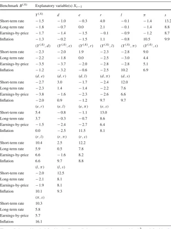
Table 1 Predictive power for dependent variableYt(A): the single benchmarking approach
BenchmarkB(A) Explanatory variable(s)Xt−1
Y(A) d e r l π s
Short-term rate −1.5 −1.0 −0.3 4.0 −0.1 −1.4 13.2
Long-term rate −1.8 −0.7 0.0 2.1 −0.1 −1.4 8.8
Earnings-by-price −1.7 −1.4 −1.5 −0.1 −0.9 −1.2 8.7
Inflation −1.3 −0.2 −1.5 1.1 −0.8 10.5 9.9
(Y(A),d) (Y(A),e) (Y(A),r) (Y(A),l) (Y(A), π) (Y(A),s)
Short-term rate −2.3 −2.0 1.9 −2.3 −2.8 9.0
Long-term rate −2.2 −1.8 0.0 −2.5 −3.0 4.4
Earnings-by-price −3.5 −3.7 −2.0 −2.8 −2.8 5.1
Inflation −1.2 −3.2 −0.6 −2.5 10.2 6.9
(d,e) (d,r) (d,l) (d, π) (d,s)
Short-term rate −2.7 3.0 −1.7 −2.4 12.0
Long-term rate −2.3 1.4 −1.4 −2.2 7.6
Earnings-by-price −3.8 −1.6 −2.3 −2.6 6.6
Inflation −2.0 0.9 −1.2 9.7 9.7
(e,r) (e,l) (e, π) (e,s)
Short-term rate 5.4 −0.8 −1.1 13.0
Long-term rate 3.7 −0.3 −0.7 8.6
Earnings-by-price −1.5 −2.4 −2.7 6.4
Inflation 0.0 −2.5 11.5 8.1
(r,l) (r, π) (r,s)
Short-term rate 10.4 2.5 12.2
Long-term rate 5.9 0.5 7.8
Earnings-by-price 6.6 −1.6 8.2
Inflation 6.6 9.7 8.8
(l, π) (l,s)
Short-term rate −2.0 12.5
Long-term rate −2.1 8.1
Earnings-by-price −1.9 8.1
Inflation 10.1 9.3
(π,s)
Short-term rate 10.3
Long-term rate 5.8
Earnings-by-price 5.7
Inflation 16.1
The prediction problem is defined in (1). The predictive power (%) is measured byR2V as defined in (5).
The benchmarksB(A)considered are based on the short-term interest rate (A≡R), long-term interest rate
(A≡L), earnings-by-price ratio (A≡E), and consumer price index (A≡C). The predictive variables used
areXt−1, given by the dividend-by-price ratiodt−1, earnings-by-price ratioet−1, short-term interest rate
rt−1, long-term interest ratelt−1, inflationπt−1, term spreadst−1, excess stock returnYt(−A1), or the possible
variable(s) is (are) measured on the original nominal scale. The model (1) is estimated with a local-linear kernel smoother using the quartic kernel and the optimal bandwidth is chosen by cross-validation, i.e., by maximizing theR2
Vgiven by (5). Moreover, it should be kept in
mind that the nonparametric method can estimate linear functions without any bias, given that we apply a local-linear smoother. Thus, the linear model is automatically embedded in our approach.
We study the empirical findings ofR2Vvalues based on different validated scenarios shown in Table1. Overall, we find that the term spreadsis in itself the most important predictor under the different benchmarks. This remains quite the case also when combining with additional information. Inflation is another predictor that performs well when used concurrently as a benchmark. Hence, these are aspects where we focus our spotlight on in our discussion.
More specifically, if we constrain prediction to using only one-dimensional covariates, then the term spreadsis the best predictor under the short interest benchmarkB(R)with
R2V =13.2%, but also does quite well under the inflation benchmarkB(C)withR2V =9.9%.
Imposing an additional covariate toshas, in general, a decreasing effect on R2V however not substantial. Under B(R), RV2 remains in the majority of the combinations within the range 12.0–13.2%. Under other benchmarks such as, for example,B(L),syieldsR2
Vin the
range 7.6–8.8%; underB(E),R2Vlies in the range 6.4–8.7%. The two-dimensional covariates (Y(R),s),(Y(L),s)and(Y(E),s)result in lower predictive power than the previous ranges under B(R), B(L)andB(E) with, respectively, R2V values 9%, 4.4% and 5.1%; while still below the best-performing ranges,(π,s)is found slightly better underB(R),B(L)andB(E)
with, respectively,R2Vvalues 10.3%, 5.8% and 5.7% . It is worth noting that the occasional reduction in predictive power in the two-dimensional compared to the one-dimensional case is not particularly surprising as we use a fully nonparametric smoother that requires more observations than a linear regression to produce consistent estimates when fitting higher-dimensional models. Therefore, our cross-validatedR2V might rank one-dimensional better than two-dimensional models. (Note that this is not the case for a linear model estimated with OLS based on the usualR2measure which would always choose the most complex model.)
Remarkable is the case of the predictorπ, either in itself or combined with covariates
Y(C),d,e,r,l, under the inflation benchmarkB(C)leading to R2V in the range 9.7–11.5%.
In addition, when put together with the term spread, the resulting combination(π,s)under
B(C)is the clear winner reaching up toRV2 =16.1%. Given that the inflation benchmark might be the most important one for many pension product applications, this high predictive power is appealing. Under theB(R),B(L)andB(E)benchmarks, the performance of covariate πdeteriorates and, in fact, the historical average excess return in these cases surpasses the predictor-based regression model, as implied by negative R2V, unless it is combined with covariaterors.
Finally, other covariates in themselves or combined also lead to negativeRV2 values; such predictor examples includeY,d,e,land their pairwise combinations under any benchmark. On the contrary, the short-term raterindividually or combined with other covariates boosts, with a few exceptions, the predictive power of our nonparametric regression model.
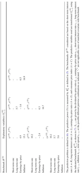
5.3 Full benchmarking approach
Table 2 Predicti v e po wer for dependent v ariable Y ( A ) t : the full benchmarking approach Benchmark B ( A ) Explanatory v ariable(s) X ( A ) t − 1 Y ( A ) d ( A ) e ( A ) r ( A ) l ( A ) π ( A ) s ( A ) Short-term rate − 1.5 4 .2 7.0 – 13.2 − 1.2 13.2 Long-term rate − 1.8 − 0.2 1 .0 8.9 – − 1.5 8 .9 Earnings-by-price − 1.7 − 2.3 – 0.3 − 1.2 0 .0 8.7 Inflation − 1.3 10.7 13.3 6 .6 10.8 – 8.9 ( Y ( A
),d
( A ))( Y ( A
),e
( A ))( Y ( A
),r
( A ))( Y ( A
),l
( A ))( Y ( A ),π ( A ))( Y ( A
),s
( A )) Short-term rate 2.7 5 .0 – 8 .7 − 2.7 8 .7 Long-term rate − 1.9 − 0.8 4 .3 – − 3.1 4 .3 Earnings-by-price − 4.1 – − 1.7 − 3.2 − 2.5 5 .0 Inflation 11.2 12.3 5 .8 10.1 – 6.0 ( d ( A
),e
( A ))( d ( A
),r
( A ))( d ( A
),l
( A ))( d ( A ),π ( A ))( d ( A
),s
( A )) Short-term rate 4.1 – 11.5 2 .6 11.5 Long-term rate − 1.2 7 .0 – − 1.8 7 .0 Earnings-by-price – − 2.8 − 3.7 − 3.2 4 .9 Inflation 11.2 9 .8 10.3 – 16.2 ( e ( A
),r
( A ))( e ( A
),l
( A ))( e ( A ),π ( A ))( e ( A
),s
Table 2 continued Benchmark B ( A ) Explanatory v ariable(s) X ( A ) t − 1 ( r ( A
),l
( A ))( r ( A ),π ( A ))( r ( A
),s
( A )) Short-term rate – – – Long-term rate – 5 .7 – Earnings-by-price 4.9 − 1.6 6 .5 Inflation 15.1 – 16.9 ( l ( A ),π ( A ))( l ( A
),s
( A )) Short-term rate 10.2 – Long-term rate – – Earnings-by-price − 2.4 6 .3 Inflation – 16.7 (π ( A
),s
( A )) Short-term rate 10.2 Long-term rate 5.7 Earnings-by-price 5.6 Inflation – The p rediction p roblem is defined in ( 6 ). The p redicti v e po wer (%) is measured by R 2 V as defined in ( 5 ). The b enchmarks B ( A )considered are b ased on the short-term interest rate ( A ≡ R ), long-term interest rate ( A ≡ L ), earnings-by-price ratio ( A ≡ E ), and consumer price inde x ( A ≡ C ). The p redicti v e v ariables used are transformed X ( A ) t − 1 using the indicated benchmark B ( A ) t − 1 as sho w n in ( 7 ). Xt − 1 are g iv en by the d iv idend-by-price ratio
dt−
1
,
earnings-by-price
ratio
et−
1
,
short-term
interest
rate
rt−
1
,
long-term
interest
rate
lt−
1
,
inflation
πt−
1
,
term
spread
st−
[image:12.439.57.327.50.619.2]is well-known that importing more structure in the estimation process can help reduce or circumvent such problems. For example, Nielsen and Sperlich (2003) investigate an additive functional structure in the context of predictability of excess stock returns (as proposed in the statistical literature by Stone1985). Their results indicate a more complex structure than additivity, as the fully nonparametric models always do better in terms of validatedR2
than the additive counterparts. Scholz et al. (2015) propose a semiparametric bias reduction method for the purpose of importing more structure based on a multiplicative correction with a parametric pilot estimate. Alternatively, Scholz et al. (2016) make use of economic theory saying that the price of a stock is driven by fundamentals and investors should focus on forward earnings and profitability. They include information on the same years’—instead of last years’—explanatories and improve predictions.
Here, we propose an extension of the study in Sect. 5.2using economic structure by adjusting both the independent and dependent variables according to the same benchmark. For example, in the full benchmarking approach with an inflation benchmark, both excess returns and covariates are expressed in terms of inflation; in pension research it is sensible to employ such a model with all returns and covariates net-of-inflation. This, in turn, provides a simple scaling when working on long-term forecasts in real terms.
In general, in our full benchmarking approach, the prediction problem is reformulated as
Yt(A)=m(Xt(−A)1)+ξt, (6)
where we use transformed predictive variables
X(t−A)1=
⎧ ⎪ ⎪ ⎨ ⎪ ⎪ ⎩
1+Xt−1
Bt(−A1)
st−1
Bt(−A)1 =
lt−1−rt−1
Bt(−A)1 ,
Yt(A)−1
(7)
whereX ∈ {d,e,r,l, π}andA ∈ {R,L,E,C}. This model can be interpreted as a way of reducing dimensionality of the estimation procedure asXt(−A)1encompasses an additional predictive variable.
Results of this empirical study are presented in Table2. We find that, in the majority of the cases, the full outruns the single benchmarking approach presented in Table1in terms ofR2V. In addition, by full benchmarking, several cases of inability of the predictor-based regression model to beat the historical average excess return are now surmounted withRV2 becoming positive. The term spreadsretains its superior predictability with perceptible improvement brought in two-dimensional settings when paired with the dividend-by-price ratiod, the earnings-by-price ratioe, the short rater, or the long ratelunder theB(C)benchmark, reaching up to a notableRV2 =18.7% when using specifically predictors(e(C),s(C)). Otherwise, as
in the single benchmarking approach, we experience some decrease in predictability when adding covariates tos, with(Y(R),s(R)),(Y(L),s(L))and(Y(E),s(E)), although resulting in positiveR2V, still performing worse underB(R),B(L)andB(E).
A few more interesting comments relating to benchmarksB(R),B(L)andB(E)are in order. We find that underB(R)andB(L)the predictive power of, respectively,l(R)andr(L), either in themselves or when combined with a common covariate such asY,d,e, π,2improves
2 For clarity, it is worth mentioning that s(R) andl(R)(and their combinations withY,d,e, π) have,
respectively, the same RV2 by construction of the transformed spread according to (7). For example,
st(R)−1 = (lt−1−rt−1)/B(R)t−1 = (1+lt−1)/(1+rt−1)−1 andlt(R)−1 = (1+lt−1)/(1+rt−1), i.e., a
considerably from the single benchmarking approach: for example, changing from predictor
l under B(R) tol(R) increases R2V from−0.1% to 13.2% or from predictorrunder B(L)
tor(L)increasesRV2 from 2.1% to 8.9%. Nevertheless, the highest predictability power for these benchmarks is close to that from the single approach originating fromsunder B(R)
andB(L); similar remark applies in the B(E) benchmark wheres(E) is the best predictor achieving at most the same level of predictability assunderB(E)in the single approach.
We turn now attention toB(C). Here, remarkable in the full approach is the contribution of the earnings-by-price ratioe(C)whose predictability, contrary to that ofeunderB(C)in the single approach, is now put on show. We find thate(C),(Y(C),e(C)),(e(C),s(C))result inR2V
of 13.3%, 12.3% and 18.7% against maximumR2Vof 10.5% (π), 10.2%(Y(C), π)and 11.5%
(e, π)from corresponding rows (benchmarkB(C)) of Table1; so there is at least one matching covariate. Notable contributions from other covariates are those of(d(C),s(C)),(r(C),s(C))
and(l(C),s(C))withRV2 of 16.2%, 16.9% and 16.7% against maximumR2Vof 9.7%(d,s)or (d, π), 9.7%(r, π)and 10.1%(l, π)from corresponding rows (benchmarkB(C)) of Table1. Overall, using earnings-by-price as an individual predictor and two-dimensional predictors that include the term spread capture the best predictive performances; the winning pair is earnings-by-price ratio and term spread.
5.4 Synopsis and further discussion
In summary, our study indicates that with single benchmarking, the spread in nominal terms has a significantly higher predictability than the price or even the earnings-by-price together with the spread. With full benchmarking though, net-of-inflation, i.e., in real terms, the earnings-by-price beats the spread, with their combination performing best. This is an important observation as benchmarking fits well in building models net-of-inflation, as discussed in Donnelly et al. (2018) and Gerrard et al. (2018,2019), while at the same time expanding to double benchmarking endows earnings with predictive power. This is a crucial implication for pension research or other long-term saving strategies, where one should look at real value and implement double benchmarking including both spread and earnings.
In addition, as part of their comprehensive analysis of a long literature including arti-cles based on different techniques, variables, and time periods, and sometimes contradicting results, Welch and Goyal (2008) find that predictive linear regressions using prominent vari-ables, including our choices, do result in poor predictability, in-sample and out-of-sample. Nevertheless, following their recommendation, we explore the possibility of an alternative model approach, here, a simple nonparametric regression model and different benchmarks. Contrary to them, our method with double benchmarking leads, as highlighted earlier, to favourable predictive results implying that nonlinear and/or nonparametric models are nec-essary to represent the complicated relationship between earnings, prices, the yield curve and the stock returns.
6 Prediction of back-transformed returns
has its own merit (as we have already discussed, for example, the short-term interest rate for classical market-timing strategies or the inflation benchmark for wealth and purchasing power issues of long-term investments); with a back-transform we lose this focus.
Keeping these points in mind, we proceed with a comparability exercise. To this end, from the stock returns in excess of general benchmarkA,Yt(A)=lnSt−lnBt(A)−1, we directly get
lnSt= ˆYt(A)+lnBt(A)−1,
whereYˆis the predicted benchmarked excess return, and thereby redefine our original vali-dation criterion (5) as
R2V =1−
t
lnSt−lnS
−t
2
t
lnSt−
lnS−t
2,
wherelnS−t is the back-transformed stock return prediction from the original leave-one-out benchmarked return prediction andlnS−tthe unconditional mean of lnS. This allows us to validate in terms ofR2
Vwith the observed lnSt. The numbers originating from the single
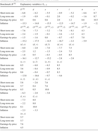
and full benchmarking approaches are summarized respectively in Tables3and4.
More specifically, we find that the term spreadsremains the single most important pre-dictor under the benchmarks B(R), B(L)andB(E) with a maximum R2V of 10.5%, while,
consistently with Kothari et al. (2006) who state that lagged earnings exhibit no predictive power for future annual returns, earnings-by-priceehave mostly negativeR2V. However, by referring to Tables1and3, we see that it becomes generally hard to predict the inflation benchmark, i.e., inflation losses somehow its good performance; the only combination of predictors that results in a positiveR2Vof 4.5% in this case is inflation together with the term
spread(π,s). This might be attributed to the persistence of inflation in later years of the
time series, i.e., the largeR2Vvalues in Table1for the benchmarkB(C)are based on a well-predicted inflation component of the transformed dependent variable. On the other hand, the predictive power of the benchmarkB(E)in Table3increases notably, indeed giving the largest
R2Vof 10.5%. The benchmarkB(L)seems to be invariant under the back-transformation, i.e., theR2Vvalues are mostly the same as in Table1, whilst the benchmarkB(R)gives generally smallerR2
V values than in Table1and seems to be performing more poorly thanB(L).
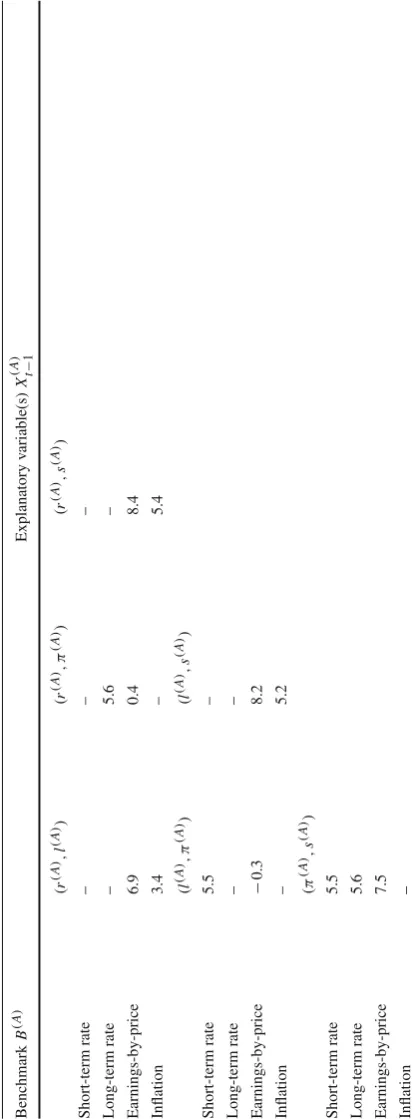
Focusing now on full benchmarking’s results in Table 4, we find that in many cases the predictive power increases, however the overall best R2V remains 10.5% for the same
model as in the single benchmarking approach in Table3. Again, the benchmarkB(L)gives similar numbers to the original full benchmarking in Table2,B(R)is slightly worse, and
B(E) performs best. The inflation benchmark B(C) performs much better than in single benchmarking (Table3), especially for the predictor variable combination of earnings-by-price and term spread(e(C),s(C))withR2
V =7.5%. The term spread is consistently the best
predictor.
Table 3 Predictive power for back-transformed dependent variable lnSt: the single benchmarking approach,
validated on original scale without benchmark in terms ofln(St)
BenchmarkB(A) Explanatory variable(s)Xt−1
Y(A) d e r l π s
Short-term rate −6.8 −6.2 −5.5 −0.9 −5.2 −6.6 8.7
Long-term rate −1.9 −0.9 −0.1 2.0 −0.2 −1.6 8.7
Earnings-by-price 0.3 0.6 0.6 2.0 1.2 0.8 10.5
Inflation −15.3 −14.0 −15.5 −12.5 −14.7 −1.9 −2.5
(Y(A),d) (Y(A),e) (Y(A),r) (Y(A),l) (Y(A), π) (Y(A),s)
Short-term rate −7.6 −7.3 −3.2 −7.6 −8.1 4.3
Long-term rate −2.4 −1.9 −0.1 −2.6 −3.2 4.3
Earnings-by-price −1.5 −1.6 0.0 −0.7 −0.7 7.0
Inflation −15.2 −17.5 −14.5 −16.7 −2.2 −5.9
(d,e) (d,r) (d,l) (d, π) (d,s)
Short-term rate −8.0 −2.0 −7.0 −7.7 7.5
Long-term rate −2.5 1.2 −1.5 −2.4 7.5
Earnings-by-price −1.8 0.5 −0.3 −0.5 8.5
Inflation −16.1 −12.7 −15.2 −2.8 −2.8
(e,r) (e,l) (e, π) (e,s)
Short-term rate 0.5 −6.0 −6.3 8.5
Long-term rate 3.6 −0.4 −0.9 8.5
Earnings-by-price 0.6 −0.4 −0.7 8.3
Inflation −13.8 −16.6 −0.7 −4.6
(r,l) (r, π) (r,s)
Short-term rate 5.8 −2.6 7.6
Long-term rate 5.7 0.4 7.6
Earnings-by-price 8.5 0.5 10.0
Inflation −6.3 −2.8 −3.8
(l, π) (l,s)
Short-term rate −7.3 8.0
Long-term rate −2.2 8.0
Earnings-by-price 0.1 10.0
Inflation −2.3 −3.3
(π,s)
Short-term rate 5.7
Long-term rate 5.7
Earnings-by-price 7.6
Table 4 Predicti v e po wer for back-transformed dependent v ariable ln St : the full benchmarking approach, v alidated on original scale without benchmark in terms of ln( St ) Benchmark B ( A ) Explanatory v ariable(s) X ( A ) t − 1 Y ( A ) d ( A ) e ( A ) r ( A ) l ( A ) π ( A ) s ( A ) Short-term rate − 6.8 − 0.8 2 .2 – 8 .7 − 6.4 8 .7 Long-term rate − 1.9 − 0.4 0 .9 8.7 – − 1.6 8 .7 Earnings-by-price 0.3 − 0.2 – 2.3 0 .9 2.0 1 0.5 Inflation − 15.3 − 1.7 1 .3 − 6.3 − 1.5 – − 3.7 ( Y ( A
),d
( A ))( Y ( A
),e
( A ))( Y ( A
),r
( A ))( Y ( A
),l
( A ))( Y ( A ),π ( A ))( Y ( A
),s
( A )) Short-term rate − 2.3 0 .1 – 4 .0 − 8.0 4 .0 Long-term rate − 2.0 − 0.9 4 .2 – − 3.2 4 .2 Earnings-by-price − 2.0 – 0.3 − 1.2 − 0.5 6 .9 Inflation − 1.1 0 .2 − 7.2 − 2.3 – − 7.0 ( d ( A
),e
( A ))( d ( A
),r
( A ))( d ( A
),l
( A ))( d ( A ),π ( A ))( d ( A
),s
( A )) Short-term rate − 0.9 – 6.9 − 2.5 6 .9 Long-term rate − 1.4 6 .9 – − 2.0 6 .9 Earnings-by-price – − 0.8 − 1.6 − 1.1 6 .8 Inflation − 1.1 − 2.7 − 2.1 – 4.6 ( e ( A
),r
( A ))( e ( A
),l
( A ))( e ( A ),π ( A ))( e ( A
),s
Table
4
continued
Benchmark
B
(
A
)
Explanatory
v
ariable(s)
X
(
A
)
t
−
1
(
r
(
A
),l
(
A
))(
r
(
A
),π
(
A
))(
r
(
A
),s
(
A
))
Short-term
rate
–
–
–
Long-term
rate
–
5
.6
–
Earnings-by-price
6.9
0
.4
8.4
Inflation
3
.4
–
5
.4
(
l
(
A
),π
(
A
))(
l
(
A
),s
(
A
))
Short-term
rate
5.5
–
Long-term
rate
–
–
Earnings-by-price
−
0.3
8
.2
Inflation
–
5.2
(π
(
A
),s
(
A
))
Short-term
rate
5.5
Long-term
rate
5.6
Earnings-by-price
7.5
Inflation
[image:18.439.58.266.55.615.2]the fact that from this back-transformation exercise the different benchmarks behave quite differently when the target is lnS insinuates that the imposed structure matters, in other words, the benchmarking has a bias-correction effect.
7 Conclusion
In this communication, we define machine learning as a working framework comprising the following summarized key ingredients: articulation, domain knowledge, final selection by validation, conduct of validation consistently with underlying statistical principles and properly channeled prior knowledge. We then apply to forecasting stock returns in excess of different benchmarks, including the inflation, long interest rate and earnings-by-price ratio to supplement the short interest rate which is by far the most commonly used in finance. Indeed, this paper expresses an interest in going beyond this as different benchmarks might be important, for example, when modelling returns in real terms (inflation benchmark) or modelling returns in excess of long-term interest rate.
We use predictors such as the dividend-by-price ratio, earnings-by-price ratio, short inter-est rate, long interinter-est rate, the term spread, the inflation, as well as the lagged excess stock return. We also investigate the option of full benchmarking, meaning that, not only returns are benchmarked, but also the covariates used to predict them. The full benchmarking approach can also be seen as an example of a dimension reduction technique, where more information is included in the nonparametric prediction without extra cost in the form of increasing prob-lem dimensionality. From this analysis, we conclude that, in real terms, the combination of earnings-by-price and long-short rate spread within our nonparametric model setting has the best predictive outcome, which is important for long-term saving strategies.
In the last part, by back-transforming the benchmarked prediction models, we study the predictability of the actual stock returns. In this case the inflation benchmark loses its good performance, however this process uncovers the predictive power of the earnings-by-price ratio benchmark, which serves as a return metric for investors, and the term spread covariate which tends to be signalling the market cycles.
Acknowledgements The authors thank two anonymous referees for their constructive comments and sugges-tions. The second author acknowledges financial support from the Cass Business School Doctoral Training Programme. The third author thanks the Institute and Faculty of Actuaries in the UK for financial support through the grant “Minimizing Longevity and Investment Risk while Optimizing Future Pension Plans”. A version of this paper has been presented at the research seminar series of the Department of Economics, Universität Graz, Austria; we thank all participants for their comments. The usual disclaimer applies.
Open Access This article is distributed under the terms of the Creative Commons Attribution 4.0 International
License (http://creativecommons.org/licenses/by/4.0/), which permits unrestricted use, distribution, and
repro-duction in any medium, provided you give appropriate credit to the original author(s) and the source, provide a link to the Creative Commons license, and indicate if changes were made.
References
Bandi, F. M., Corradi, V., & Wilhelm, D. (2016). Possibly nonstationary cross-validation. Cemmap Working Paper CWP11/16.
Bikker, J. A., Broeders, D. W. G. A., Hollanders, D. A., & Ponds, E. H. M. (2012). Pension funds’ asset
allocation and participant age: A test of the life-cycle model.Journal of Risk and Insurance,79, 595–
Burman, P., Chow, E., & Nolan, D. (1994). A cross-validatory method for dependent data.Biometrika,81, 351–358.
Chen, L., Da, Z., & Priestley, R. (2012). Dividend smoothing and predictability.Management Science,58,
1834–1853.
Cheng, T., Gao, J., & Linton, O. (2018). Multi-step non- and semi-parametric predictive regression for short and long horizon stock return prediction. Cemmap Working Paper CWP03/18.
Dahlhaus, R. (1997). Fitting time series models to nonstationary processes.The Annals of Statistics,25, 1–37.
Donnelly, C., Guillen, M., Nielsen, J. P., & Pérez-Marín, A. M. (2018). Implementing individual savings
decisions for retirement with bounds on wealth.ASTIN Bulletin,48, 111–137.
Doukhan, P. (1994).Mixing. New York: Springer.
Elliott, G., Gargano, A., & Timmermann, A. (2013). Complete subset regressions.Journal of Econometrics,
177, 357–373.
Favero, C. A., Gozluklu, A. E., & Tamoni, A. (2011). Demographic trends, the dividend-price ratio, and
the predictability of long-run stock market returns.Journal of Financial and Quantitative Analysis,46,
1493–1520.
Gerrard, R., Guillén, M., Nielsen, J. P., & Pérez-Marín, A. M. (2014). Long-run savings and investment strategy
optimization.The Scientific World Journal,2014, 1–13.
Gerrard, R., Hiabu, M., Kyriakou, I., & Nielsen, J. P. (2018). Self-selection and risk sharing in a modern world
of life-long annuities.British Actuarial Journal,23, 1–12.
Gerrard, R., Hiabu, M., Kyriakou, I., & Nielsen, J. P. (2019). Communication and personal selection of pension
saver’s financial risk.European Journal of Operational Research,274, 1102–1111.
Guillén, M., Jarner, S. F., Nielsen, J. P., & Pérez-Marín, A. M. (2014). Risk-adjusted impact of administrative
costs on the distribution of terminal wealth for long-term investment.The Scientific World Journal,2014,
1–12.
Guillén, M., Konicz, A. K., Nielsen, J. P., & Pérez-Marín, A. M. (2013a). Do not pay for a Danish interest
guarantee. The law of the triple blow.Annals of Actuarial Science,7, 192–209.
Guillén, M., Nielsen, J. P., Pérez-Marín, A. M., & Petersen, K. S. (2013b). Performance measurement of
pension strategies: A case study of Danish life-cycle products.Scandinavian Actuarial Journal,2013,
49–68.
Györfi, L., Härdle, W., Sarda, P., & Vieu, P. (1990).Nonparametric curve estimation from time series. Lecture
notes in statistics. Heidelberg: Springer.
Hansen, B. E. (2006). Uniform convergence rates for kernel estimation with dependent data.Econometric
Theory,24, 726–748.
Harvey, D., Leybourne, S., Sollis, R., & Taylor, R. (2018). Detecting regimes of predictability in the U.S. equity premium. Essex Finance Center Working Paper No 37: 10-2018.
Kothari, S. P., Lewellen, J., & Warner, J. B. (2006). Stock returns, aggregate earnings surprises, and behavioral
finance.Journal of Financial Economics,79, 537–568.
Li, Q., & Racine, J. S. (2007).Nonparametric econometrics. Princeton: Princeton University Press.
Masry, E. (1996). Multivariate regression estimation local polynomial fitting for time series.Stochastic
Pro-cesses and their Applications,65, 81–101.
Merton, R. C. (2014). The crisis in retirement planning.Harvard Business Review,92, 43–50.
Nielsen, J. P., & Sperlich, S. (2003). Prediction of stock returns: A new way to look at it.ASTIN Bulletin,33,
399–417.
Owadally, I., Haberman, S., & Gómez Hernández, D. (2013). A savings plan with targeted contributions.
Journal of Risk and Insurance,80, 975–1000.
Pesaran, H., & Timmermann, A. (2002). Market timing and return predictability under model instability.
Journal of Empirical Finance,8, 495–510.
Rapach, D. E. & Wohar, M. (2004). Structural change and the predictability of stock returns. St. Louis University and University of Nebraska at Omaha Working Paper.
Resnick, B. G., & Shoesmith, G. L. (2002). Using the yield curve to time the stock market.Financial Analysts
Journal,58, 82–90.
Robinson, P. M. (1983). Nonparametric estimators for time series.Journal of Time Series Analysis,4, 185–207.
Scholz, M., Nielsen, J. P., & Sperlich, S. (2015). Nonparametric prediction of stock returns based on yearly
data: The long-term view.Insurance: Mathematics and Economics,65, 143–155.
Scholz, M., Sperlich, S., & Nielsen, J. P. (2016). Nonparametric long term prediction of stock returns with
generated bond yields.Insurance: Mathematics and Economics,69, 82–96.
Shiller, R. J. (1989).Market Volatility. Cambridge: MIT Press.
Stone, C. J. (1985). Additive regression and other nonparametric models.Annals of Statistics,13, 689–705.
Valkanov, R. (2003). Long-horizon regressions: Theoretical results and applications.Journal of Financial
Vogt, M. (2012). Nonparametric regression for locally stationary time series.The Annals of Statistics,40, 2601–2633.
Welch, I., & Goyal, A. (2008). A comprehensive look at the empirical performance of equity premium
pre-diction.The Review of Financial Studies,21, 1455–1508.