TRANSFERABILITY OF NEURAL NETWORK APPROACHES FOR LOW-RATE ENERGY
DISAGGREGATION
David Murray
?Lina Stankovic
?Vladimir Stankovic
?Srdjan Lulic
†Srdjan Sladojevic
†?
Dept. Electronic & Electrical Engineering, University of Strathclyde, Glasgow, United Kingdom
†
PanonIT, Novi Sad, Serbia
ABSTRACT
Energy disaggregation of appliances using non-intrusive load mon-itoring (NILM) represents a set of signal and information process-ing methods used for appliance-level information extraction out of a meter’s total or aggregate load. Large-scale deployments of smart meters worldwide and the availability of large amounts of data, moti-vates the shift from traditional source separation and Hidden Markov Model-based NILM towards data-driven NILM methods. Further-more, we address the potential for scalable NILM roll-out by tack-ling disaggregation complexity as well as disaggregation on houses which have not been ’seen’ before by the network, e.g., during train-ing. In this paper, we focus on low rate NILM (with active power meter measurements sampled between 1-60 seconds) and present two different neural network architectures, one, based on convolu-tional neural network, and another based on gated recurrent unit, both of which classify the state and estimate the average power con-sumption of targeted appliances. Our proposed designs are driven by the need to have a well-trained generalised network which would be able to produce accurate results on a house that is not present in the training set, i.e., transferability. Performance results of the de-signed networks show excellent generalization ability and improve-ment compared to the state of the art.
Index Terms— Energy analytics, non-intrusive load
monitor-ing, energy disaggregation, neural networks, deep learning
1. INTRODUCTION
Non-Intrusive Load Monitoring (NILM) refers to identifying and ex-tracting individual appliance consumption patterns from aggregate consumption readings, to estimate how much each appliance is con-tributing to the total load. This problem has been researched for over 30 years [1] and has become an active area of research again recently due to ambitious energy efficiency goals, smart homes/buildings, and large-scale smart metering deployment programmes worldwide.
Different approaches have been proposed for NILM, using vari-ous signal processing and machine learning techniques (reviews can be found in [2, 3]). Approaches proposed include include Hidden Markov Models (HMM)-based methods and their variants (see, e.g., [4, 5]), signal processing methods, such as dynamic time warping [6, 7, 8], single-channel source separation [9], graph signal process-ing [10, 11], decision trees [6], support vector machines with K-means [12], genetic algorithms [13, 14] and neural networks [15].
The recent increase in availability of load data, e.g., [9, 16, 17], for model training has igniteddata-drivenapproaches, such as deep neural networks (DNNs) using both convolutional neural network (CNN) and recurrent neural network (RNN) architectures [18, 19, 20, 21]. Currently, DNN-based NILM relies on creating a new net-work for each house and each appliance. With the availability of
Table 1. DNN-based NILM methods used in previous papers (Dataset abbreviations: UK-DALE = UK-D, Prv. = Private.
Paper Year Datasets Synthetic Best Architecture Data
[24] 2016 UK-D No LSTM
[18] 2015 UK-D Yes Denoising Autoencoder [20] 2017 UK-D, REDD, Prv. No LSTM
[21] 2018 UK-D No Deep CNN [22] 2016 UK-D, REDD No CNN
[23] 2017 Prv. Yes Stacked Denoising Autoencoder [25] 2015 REDD Yes LSTM
[26] 2015 REDD Yes HMM-DNN
a sufficient and good training dataset, these networks perform well as they are highly targeted, but if NILM is to become widespread and scalable, networks will need to be trained on a wide range of electrical load signatures. As such, the challenge is to design a sin-gle network to accurately disaggregate any appliance across multiple “unseen” houses, i.e., houses not present in the training dataset.
Though the previous DNN-based approaches [18, 19, 20, 21, 22, 23, 24] demonstrated competitive results, they do not fully exploit the DNN potential. Indeed, the approaches of [18] and [19] are lim-ited by generation of synthetic activations, which do not necessarily capture “noise” well, here defined as unknown simultaneous appli-ance use, usually present in the dataset. In [25, 26], an long short-term memory (LSTM) & DNN-HMM approach was used to rebuild the appliance signal but due to the difference in aggregate and sub-metered sampling rates in the REDD dataset, synthetic data was used exclusively in both papers by summing all sub-meters; this limits the amount of noise as appliances not sub-metered would be excluded. [20] uses real “noisy” dataset, but requires thousands of epochs to generate accurate results, which is not a feasible approach for online disaggregation, while the architecture of [21] contains large number (i.e., 44) layers designed only for identification of appliance state, without generating disaggregation or load consumption estimations. Table 1 summarises the state-of the-art DNN-based NILM meth-ods. Though prior work considered transferability across houses within the same dataset (e.g., [18, 19]), only [27] has looked at cross dataset evaluation (using curve fitting and DBSCAN to gen-erate a generic model for each appliance), i.e., transferability across datasets. This is particularly challenging due to the large variation in sampling rates, appliances, usage patterns, climate, age (differ-ent energy labels) and electrical specifications (e.g., voltage, phase) across datasets. Cross-dataset transferability is very much needed in order to be able to use the developed models at scale.
The main contributions of this paper are:
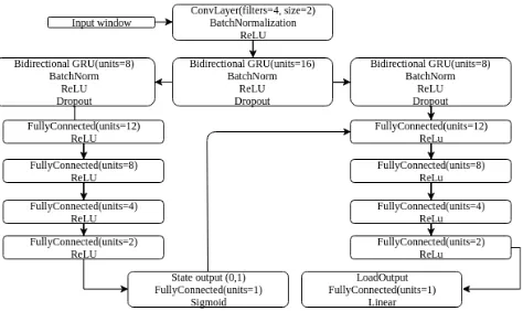
Fig. 1. Proposed GRU Network Architecture.
AND estimate the contribution to the total load of a specific appli-ance. Our approach addresses these problemsinseparablywith flow of information from the classification part of the network to the load estimation part. This is in contrast to previous work that focused on binary classification of appliance state (ex. [19, 20, 21]) or estima-tion of appliance load mainly (ex. [22, 18]).
(b) The proposed architectures are designed to facilitate success-ful transfer learning between very distinct datasets.
(c) Our proposed networks represent a significant reduction in complexity (the number of trainable parameters) compared to pre-vious approaches [18, 19, 20, 21, 22], even though our proposed networks are tested on arguably more challenging real datasets.
(d) We do not make use of synthetic data and perform both train-ing and testtrain-ing onbalanceddata to avoid the issue of bias due to lack of appliance activations, which is a feature of many NILM datasets. In order to demonstrate transferability, we resort to three datasets, namely UK REFIT [17] and UK-DALE [16], which we expect to have similar appliances, as well as US REDD [9], whose appliances are different in terms of electrical signatures, as com-pared to UK appliances.
2. PROPOSED NETWORK ARCHITECTURES
We introduce two networks, both of which are suited to processing temporal data: (1) a Gated Recurrent Unit (GRU) architecture, as shown in Figure 1, and (2) a Convolutional Neural Network (CNN) architecture, as shown in Figure 2. Both architectures remain pur-posely simple with a two-branch layout, with the side branch con-sidering state estimation and feeding it back to the main branch to assist with consumption estimation.
[image:2.612.58.295.71.212.2] [image:2.612.317.546.74.200.2]It is worth noting that prior work has generally focused on ei-ther state or consumption estimation, using a single-branch network [20, 21, 22], or attempting to rebuild the signal hence generating both state and consumption as an output [18, 19, 23, 24]. In the lat-ter, an autoencoder network is used where the network takes in an aggregate window and attempts to rebuild the target appliance sig-nal only; these network types require a large amount of labelled data and generally make use of synthetic data. In addition, each of our networks differs from the literature, by training on fewer epochs or by having many less trainable parameters.
The GRU is a variant of the LSTM unit, especially designed for time series data to handle the vanishing gradient problem of net-works. As such, they are designed, as LSTM, to ‘remember’ pat-terns within data, but are more computationally efficient. GRUs
Fig. 2. Proposed CNN Network Architecture.
have fewer parameters and thus may train faster or need less data to generalize. Therefore, a GRU is more suited to online learning and processing than the LSTM unit. The specific variation used in this work is the original version, proposed in [28], using an NVidia CUDA Deep Neural Network library (CuDNN) accelerated version and implemented in Keras (CuDNNGRU). The GRU network con-tains 4,861 parameters, out of which 4,757 are trainable and 104 non-trainable, i.e., hyper-parameters.
The proposed CNN consists of Conv1D (Keras) layers. 1D convolutional layers look at sub-samples of the input window and decide if the sub-sample is valuable. The CNN network contains 28,696,641 parameters, out of which 28,696,385 are trainable, and 256 non-trainable, hyper-parameters.
In both proposed networks, we make use of the ReLU func-tion [29] as the network activafunc-tion. This activafunc-tion is monotonic and half rectified, that is, any negative values are assigned to zero. This has the advantage of not generating vanishing gradients, exploding gradients or saturation. However, ReLU activations can cause dead neurons; we therefore use dropout to help mitigate the effect of dead neurons which may have been generated during training. Both pro-posed networks also use sigmoid activations for the state estimation and linear activations for the power estimation. The sigmoid func-tion is used as it only outputs between 0 and 1, thus ideal for the probability that the appliance is on or off; in our networks, we as-sume a value greater than 0.5 to be on and anything below to be off. Linear activations can be any value and therefore are the best when estimating power. Both networks are implemented using the TensorFlow wrapper library Keras using Python3.
3. TRAINING OF PROPOSED NETWORKS
We train the proposed networks using REDD and REFIT datasets, both containing sub-metered data. Note that sampling rates in these two datasets are different. To account for this, we pre-processed all data down to 1 second (using forward filling), then back to uniform 8 second intervals. Data was standardised by subtracting the mean, then dividing by the standard deviation.
We train on houses, except House 2, in both REDD and REFIT datasets, for the entire duration of the respective datasets. Testing is then performed on unseen House 2 in REDD and House 2 in RE-FIT, as well as UK-DALE House 1. The latter was used as it was monitored for the longest period of time. Details of houses used for training each appliance model are shown in Table 2.
Fig. 3. Aggregate load measurements for a typical day for Houses 2 in REFIT and REDD datasets and House 1 UK-DALE, showing relatively higher noise levels for UK REFIT and UK-DALE houses.
Table 2. Appliances and Houses Used REDD REFIT
Appliance Houses Houses Window Size (samples) On State (Watts) MW 1, 2, 3 2, 6, 8, 17 90 (12 mins) >100
DW 1, 2, 3, 4 2, 3, 6, 9 300 (40 mins) >25
FR 1, 2, 3, 6 2, 5, 9, 15, 21 800 (1.78 hours) >80
WM 2, 3, 10, 11, 17 300 (40 mins) >25
On the other hand, the REFIT and UK-DALE datasets are similar in complexity with both having multiple large appliance activations with a complex low consumption noise level at below 500 watts.
Four models are trained, one for each target appliance: dish-washer (DW), refrigerator (FR), microwave (MW) and washing ma-chine (WM). As each appliance has a different duty cycle, windows were chosen to capture a significant portion of a single activation, shown in Table 2 along with the watt thresholds, obtained using training data, and are used to decide if the appliance is deemed to be on, i.e., if the threshold was exceeded.
Input data was balanced to avoid a training bias within the net-works, by limiting the majority class to that of the minority class. Limiting the majority class was done by selecting samples at ran-dom, which resulted in a 50/50 split of the data. Validation data was then generated from randomly sampling 10% of training data. Each network was trained to 10 epochs with early stopping moni-toring “Validation Loss”; if this failed to improve after 2 epochs the best performing network weights were used. Both networks used binary cross entropy as the loss function for state classification, for consumption the CNN uses mean square error (MSE) and the GRU logcosh. The CNN uses the stochastic gradient descent (SGD) opti-miser and the GRU uses RMSprop.
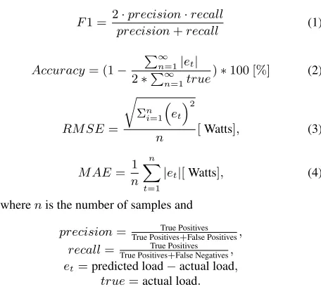
Four performance metrics are used, F1-score (state prediction), Accuracy, Root MSE (RMSE) & Mean Absolute Error (MAE)
(con-F1-Score Accuracy [%] RMSE [W] MAE [W]
Appliance CNN GRU CNN GRU CNN GRU CNN GRU
Microwave 0.95 0.95 76.4% 55.7% 165.73 252.17 68.02 127.79
Dishwasher 0.71 0.74 71.4% 76.3% 185.72 136.79 119.35 98.90
[image:3.612.318.557.161.208.2]Refrigerator 0.67 0.67 83.5% 53.9% 16.17 31.15 10.14 28.31
Table 3. Testing on “unseen” House 2, after training the networks on all other REDD houses.
F1-Score Accuracy [%] RMSE [W] MAE [W]
Appliance CNN GRU CNN GRU CNN GRU CNN GRU
Microwave 0.82 0.87 68.7% 65.6% 88.75 107.57 35.49 39.08
Dishwasher 0.82 0.82 82.9% 84.8% 200.98 211.78 82.74 73.53
Refrigerator 0.93 0.85 76.9% 64.1% 14.77 23.94 8.56 13.30
[image:3.612.330.558.281.485.2]Washing Mac 0.79 0.86 71.8% 68.9% 176.22 190.05 71.99 79.33
Table 4. Testing on “unseen” REFIT House 2, after training the networks on all other REFIT houses.
sumption estimation), which frequently appear in literature:
F1 = 2·precision·recall
precision+recall (1)
Accuracy= (1−
P∞
n=1|et| 2∗P∞
n=1true
)∗100 [%] (2)
RM SE=
r
Σn i=1
et
2
n [Watts], (3)
M AE= 1
n
n
X
t=1
|et|[Watts], (4)
wherenis the number of samples and
precision= True Positives True Positives+False Positives, recall= True PositivesTrue Positives+False Negatives, et=predicted load−actual load,
true=actual load.
The testing data was also balanced to avoid artificially improving scores; that is, in NILM datasets there is a higher likelihood that an appliance will be in an off state than it will be on (fridges and freezer being the exception). For example, a microwave may only be used once or twice per day or around 0.14% of a day. Therefore with unbalanced testing data, a network that only predicts the microwave in the off state will score well assuming that the microwave is used infrequently. Therefore, balancing the test data clearly shows the network is working well if it has an F1-score above 0.5.
[image:3.612.56.298.378.434.2]Fig. 4. Typical appliance signatures for MW, DW and FR across REDD, REFIT and UK-DALE datasets.
4. RESULTS
In this section, we demonstrate our networks’ ability to transfer across datasets. This real-world test shows the ability of the net-work to handle completely unknown appliances, duty cycles and consumption - see, for example, Figure 4.
We first present the results when the models are trained using only REFIT houses (as per Table2), and tested on House 2 from the REDD dataset. This is shown in Table 5. Compared to Table 3, we can observe a drop in performance for MW and DW, due to a difference in make/models of appliances between UK houses and the US house. Similar conclusions can be made from Table 6, where we show results when the models are trained using only REDD houses and tested on one REFIT house.
Note that in Table 6, the accuracy of Fridge is missing due to the window size selection; that is, with this window size, in the REDD dataset, there is always a fridge that is on, which means transferabil-ity between REDD to REFIT is biased to predicting the fridge always being on. This can be seen in Fig. 4, where the REDD fridge has a considerably smaller duty cycle than in the REFIT and UK-DALE datasets. This can be remedied by choosing a smaller window size; however in real-world applications this would only become apparent after testing, and multiple fridge networks may have to be generated. Table 7 shows the results of training on REFIT houses and test-ing on unseen UK-DALE House 1. The UK-DALE dataset is similar to the REFIT dataset as it is also UK based, therefore has similar appliance types. This is reflected in the scoring metrics, as it has minimal performance drop compared to Table 4.
When comparing state estimation and consumption estimation performance of the proposed CNN and GRU networks across all re-sults, we observe that they both perform similarly.
Though the metrics used are similar to those in the NILM litera-ture, we cannot directly compare our consumption estimation results with the literature because the network outputs are different. How-ever, as an indication of classification performance, [18] achieves F1 scores of 0.26 for MW, 0.74 for DW and 0.87 for FR when training on UK-DALE and testing on an unseen house also in the UK-DALE dataset. Our cross-dataset results in Table 7 show superior F1 perfor-mance for MW and FR. Comparing results for House 2 REDD, i.e., Tables 3 and 5, our best F1 scores show similar results as [19] best scores for MW (0.95), better for FR (1 vs 0.94) but slightly worse for DW (0.74 vs 0.82).
F1-Score Accuracy [%] RMSE [W] MAE [W]
Appliance CNN GRU CNN GRU CNN GRU CNN GRU
Microwave 0.41 0.49 64.1% 54.7% 120.01 103.71 90.96 39.26
Dishwasher 0.44 0.57 50.2% 39.6% 305.22 284.34 183.27 222.34
[image:4.612.52.302.71.207.2]Refrigerator 1.00 0.98 76.0% 65.5% 44.44 59.92 38.42 55.11
Table 5. Training on REFIT houses only and testing on unseen House 2 from REDD.
F1-Score Accuracy RMSE [W] MAE [W]
Appliance CNN GRU CNN GRU CNN GRU CNN GRU
Microwave 0.70 0.78 47.9% 50.8% 114.89 100.17 59.20 55.82
Dishwasher 0.80 0.62 62.8% 54.0% 431.61 386.91 179.83 222.43
[image:4.612.314.559.72.112.2]Refrigerator 0.67 0.67 – – 68.97 56.57 63.73 53.37
Table 6. Training on REDD houses only and testing on unseen House 2 from REFIT.
F1-Score Accuracy RMSE [W] MAE [W]
Appliance CNN GRU CNN GRU CNN GRU CNN GRU
Microwave 0.79 0.7 77.3% 65.11% 66.96 144.46 41.30 63.70
Dishwasher 0.21 0.46 44.1% 52.09% 43.09 44.62 29.08 24.97
[image:4.612.319.559.167.208.2]Refrigerator 1 0.69 82.0% 73.08% 14.38 19.56 11.15 16.69
Table 7. Training on REFIT houses only and testing on unseen UK-DALE House 1.
5. CONCLUSION
In this paper, we address one of the biggest NILM challenges that is yet to be demonstrated and hence limiting commercial take-up: scalability. This is reflected in performance vs complexity trade-off of NILM solutions and the ability to disaggregate appliance loads, which have previously not been seen (or trained) by the NILM solution, i.e., transferability. Driven by the increasing availability of smart meter data, we thus design and propose two data-driven deep learning based architectures that perform state estimation and classification estimation inseparably, and can generalize well across datasets. We show the ability of our trained CNN- and GRU-based networks to accurately predict state and consumption across 3 publicly available datasets, commonly used in the literature. We show that our proposed trained networks have the ability to trans-fer well across datasets with minimal performance drop, compared to the baseline when we train and test on the same dataset, albeit on an unseen household within the same dataset. Both GRU- and CNN-based networks show similar performance but the GRU-based network has fewer trainable parameters and is thus less complex than the CNN-based network.
6. ACKNOWLEDGEMENTS
[image:4.612.318.557.264.304.2]7. REFERENCES
[1] G. W. Hart, “Nonintrusive appliance load monitoring,” Pro-ceedings of the IEEE, vol. 80, no. 12, pp. 1870–1891, 1992. [2] A. Zoha, A. Gluhak, M. Imran, and S. Rajasegarar,
“Non-Intrusive Load Monitoring Approaches for Disaggregated En-ergy Sensing: A Survey,”Sensors, vol. 12, no. 12, pp. 16838– 16866, 12 2012.
[3] M. Zeifman and K. Roth, “Nonintrusive appliance load moni-toring: Review and outlook,”IEEE Transactions on Consumer Electronics, vol. 57, no. 1, pp. 76–84, 2 2011.
[4] H. Gonc¸alves, A. Ocneanu, and M. Berg´es, “Unsupervised dis-aggregation of appliances using aggregated consumption data,” in1st KDD Workshop on Data Mining Applications in Sustain-ability (SustKDD), 2011.
[5] O. Parson, S. Ghosh, M. Weal, and A. Rogers, “An unsuper-vised training method for non-intrusive appliance load moni-toring,”Artificial Intelligence, vol. 217, pp. 1–19, 12 2014. [6] J. Liao, G. Elafoudi, L. Stankovic, and V. Stankovic,
“Non-intrusive appliance load monitoring using low-resolution smart meter data,” in2014 IEEE International Conference on Smart Grid Communications (SmartGridComm). 11 2014, pp. 535– 540, IEEE.
[7] G. Elafoudi, L. Stankovic, and V. Stankovic, “Power disaggre-gation of domestic smart meter readings using dynamic time warping,” in ISCCSP 2014 - 6th International Symposium on Communications, Control and Signal Processing, Proceed-ings, 2014, pp. 36–39.
[8] A. Cominola, M. Giuliani, D. Piga, A. Castelletti, and A. E. Rizzoli, “A Hybrid Signature-based Iterative Disaggregation algorithm for Non-Intrusive Load Monitoring,” Applied En-ergy, vol. 185, pp. 331–344, 1 2017.
[9] J. Z. Kolter and M. J. Johnson, “REDD: A Public Data Set for Energy Disaggregation Research,” inSustKDD workshop on Data Mining Applications in Sustainability, 2011, pp. 1–6. [10] K. He, L. Stankovic, J. Liao, and V. Stankovic, “Non-Intrusive
Load Disaggregation Using Graph Signal Processing,” IEEE Transactions on Smart Grid, vol. 9, no. 3, pp. 1739–1747, 5 2018.
[11] B. Zhao, L. Stankovic, and V. Stankovic, “On a Training-Less Solution for Non-Intrusive Appliance Load Monitoring Using Graph Signal Processing,” IEEE Access, vol. 4, pp. 1784– 1799, 2016.
[12] H. Altrabalsi, V. Stankovic, J. Liao, and L. Stankovic, “Low-complexity energy disaggregation using appliance load mod-elling,”AIMS Energy, vol. 4, no. 1, pp. 1–21, 2016.
[13] D. Egarter, A. Sobe, and W. Elmenreich, “Evolving Non-Intrusive Load Monitoring,” in Lecture Notes in Computer Science, pp. 182–191. Springer, 2013.
[14] Z. Guanchen, G. Wang, H. Farhangi, and A. Palizban, “Res-idential electric load disaggregation for low-frequency utility applications,” in2015 IEEE Power & Energy Society General Meeting. 7 2015, pp. 1–5, IEEE.
[15] A. G Ruzzelli, C. Nicolas, A. Schoofs, and G. M P O’Hare, “Real-Time Recognition and Profiling of Appliances through a Single Electricity Sensor,” in2010 7th Annual IEEE Communi-cations Society Conference on Sensor, Mesh and Ad Hoc Com-munications and Networks (SECON). 6 2010, pp. 1–9, IEEE.
[16] J. Kelly and W. Knottenbelt, “The UK-DALE dataset, do-mestic appliance-level electricity demand and whole-house de-mand from five UK homes,”Scientific Data, vol. 2, 3 2015.
[17] D. Murray, L. Stankovic, and V. Stankovic, “An electrical load measurements dataset of United Kingdom households from a two-year longitudinal study,”Scientific Data, vol. 4, 2017. [18] J. Kelly and W. Knottenbelt, “Neural NILM,” inProceedings
of the 2nd ACM International Conference on Embedded Sys-tems for Energy-Efficient Built Environments - BuildSys ’15, New York, New York, USA, 2015, pp. 55–64, ACM Press.
[19] P. P. M. d. Nascimento, Applications of Deep Learning Tech-niques on NILM, Ph.D. thesis, COPPE/UFRJ, 2016.
[20] J. Kim, T.-T.-H. Le, and H. Kim, “Nonintrusive Load Monitor-ing Based on Advanced Deep LearnMonitor-ing and Novel Signature,”
Computational Intelligence and Neuroscience, vol. 2017, pp. 1–22, 2017.
[21] K. S. Barsim and B. Yang, “On the Feasibility of Generic Deep Disaggregation for Single-Load Extraction,” arXiv preprint, 2 2018.
[22] C. Zhang, M. Zhong, Z. Wang, N. Goddard, and C. Sutton, “Sequence-to-point learning with neural networks for nonin-trusive load monitoring,”The Thirty-Second AAAI Conference on Artificial Intelligence, 2018.
[23] F. C. C. Garcia, C. M. C. Creayla, and E. Q. B. Macabebe, “Development of an Intelligent System for Smart Home En-ergy Disaggregation Using Stacked Denoising Autoencoders,”
Procedia Computer Science, vol. 105, pp. 248–255, 2017. [24] W. He and Y. Chai, “An Empirical Study on Energy
Disag-gregation via Deep Learning,” inProceedings of the 2016 2nd International Conference on Artificial Intelligence and Indus-trial Engineering (AIIE 2016), Paris, France, 2016, Atlantis Press.
[25] L. Mauch and B. Yang, “A new approach for supervised power disaggregation by using a deep recurrent LSTM network,” in
2015 IEEE Global Conference on Signal and Information Pro-cessing (GlobalSIP). 12 2015, pp. 63–67, IEEE.
[26] L. Mauch and B. Yang, “A novel DNN-HMM-based approach for extracting single loads from aggregate power signals,” in
2016 IEEE International Conference on Acoustics, Speech and Signal Processing (ICASSP). 3 2016, pp. 2384–2388, IEEE. [27] B. Humala, A. S. U. Nambi, and V. R. Prasad,
“Universal-NILM: A Semi-supervised Energy Disaggregation Framework using General Appliance Models,” inProceedings of the Ninth International Conference on Future Energy Systems - e-Energy ’18, New York, New York, USA, 2018, pp. 223–229, ACM Press.
[28] K. Cho, B. van Merrienboer, C. Gulcehre, D. Bahdanau, F. Bougares, H. Schwenk, and Y. Bengio, “Learning Phrase Rep-resentations using RNN Encoder-Decoder for Statistical Ma-chine Translation,”arXiv preprint, 6 2014.