On the robust estimation of small failure probabilities
for strong non-linear models
Matthias Faesa,∗, Jonathan Sadeghic, Matteo Broggib, Marco de Angelisc, Edoardo Patellic, Michael Beerb,c,d, David Moensa
aKU Leuven, Department of Mechanical Engineering, Technology campus De Nayer, Jan De Nayerlaan 5, St.-Katelijne-Waver, Belgium
bLeibniz Universit¨at Hannover, Institute for Risk and Reliability, Callinstrasse 34, Hannover, Germany
cUniversity of Liverpool, Institute for Risk and Uncertainty, Peach Street, L69 7ZF Liverpool, United Kingdom
dTongji University, International Joint Research Center for Engineering Reliability and Stochastic Mechanics, Shanghai 200092, China
Abstract
Structural reliability methods are nowadays a cornerstone for the design of
robustly performing structures, thanks to advancements in modeling and
simulation tools. Monte-Carlo based simulation tools have been shown to
provide the necessary accuracy and flexibility. While standard Monte-Carlo
estimation of the probability of failure is not hindered in its applicability by
approximations or limiting assumptions, it becomes computationally
unfea-sible when small failure probability needs to be estimated, especially when
the underlying numerical model evaluation is time consuming.
In this case, variance reduction techniques are commonly employed,
al-lowing for the estimation of small failure probabilities with a reduced number
of samples and model calls. As a competing approach to variance reduction
∗Corresponding author
techniques, surrogate models can be used to substitute the
computation-ally expensive model and performance function with an easy to evaluate
nu-merical function calibrated through a supervised learning procedure. Both
these tools can provide accurate results for structural application. However,
particular care should be taken into account when the reliability problems
deal with high dimensional or strongly non-linear structural performances.
In this work, we compare the performance of the most recent
state-of-the-art advance Monte-Carlo techniques and surrogate models when applied to
strongly non-linear performance functions. This will provide the analysts
with an insight to the issues that could arise in these challenging problems
and help to decide with confidence on which tool to select in order to achieve
accurate estimation of the failure probabilities within feasible times with
their available computational capabilities.
Keywords: Kriging, Interval Predictor, Failure Probability, surrogate modeling, model emulation
1. INTRODUCTION
Nowadays, the design of engineering structures, systems or networks is
largely based on computer based work flows. These work flows are
particu-larly crafted on the application of numerical methods for the solution of the
sets of differential equations that model and describe the physical processes
involved in such applications. However, since these methods do not
tradi-tionally account for the inherent and unavoidable non-deterministic nature
of the modeled processes, a large degree of over-conservatism needs to be
no longer capable of fulfilling its initial design purpose). This conservatism
might possibly cancel out the improvements achieved through the numerical
optimization procedures.
Therefore, nowadays engineering design processes should account for the
non-determinism in e.g., the mechanical properties of the used materials, the
loading of the structure, etc. Then, based on a solid mathematical
descrip-tion of these properties, the reliability of these structures can be effectively
assessed and included even in the earliest design stages. In practice, the
assessment of the reliability is made by computing the probability that the
structure is failing to satisfy its initial design requirements given the
ran-domness or uncertainty on its structural properties and functional loading
environment. Consider a modelm :Rnx 7→
Rny that predicts the structural
responsesy ∈ Y ⊂Rny, based on a vector of parametersx∈ X ⊂
Rnx of the
model. X is herein the set of admissible model parameters, As the actual
value of the model parameters inx is either inherently variable, unknown or
both, also the prediction of the model responses y is also not deterministic. In a probabilistic context, both quantities are modeled as a random vectors,
and their realizations are respectively distributed according to the
probabil-ity densprobabil-ity functions fX(x) and fY(y). In that case, the probability of
failure Pf , that is, the probability that the structure does not satisfy its
per-formance requirements, is computed as the probability of a model response
belonging to the failure domain F:
Pf =P(y∈ F) = Z
Rny
with IF :Rny 7→ {0,1}the indicator function, which is defined as:
IF =
0 ⇐⇒ Y ∈ {y|y=m(x), x∈ X, g(y)>0}
1 ⇐⇒ Y ∈ {y|y=m(x), x∈ X, g(y)≤0}
(2)
withg(y) :Rny 7→
Rthe so-called limit-state function that indicates whether
or not the structure satisfies a predefined performance. In practice, the
considered model m() can be high-dimensional in terms of parameters and
responses. Moreover, the indicator function IF is in most cases non-linear.
Therefore, it is generally intractable to obtain an analytical solution to the
integral in eq. (1). As a solution hereto, simulation methods are commonly
applied to approximate the probability of failure, based on a large number of
realizations of the non-deterministic parameters x and obtaining the corre-sponding model responsesy. The most common approach is to follow Monte
Carlo integration of eq. (1). However, when a sufficiently accurate
estima-tion of a very small Pf (i.e. Pf <10−3) is desired (e.g. with a coefficient of
variation of less than 5%), a very high number of evaluations of the model
m() is typically needed, which is computationally intractable in case even
medium-scaled numerical models are considered. As an attempt to
allevi-ate this problem, advanced Monte Carlo methods, also known as variance
reduction techniques, such as Line Sampling [1], Subset simulation [2], and
more recently SubSet-∞[3] have been introduced. These methods have been
applied to large scale problems in e.g. [4, 5, 6], and the gain in computational
efficiency has been numerously illustrated (e.g., [7]). Although these highly
advanced methods typically require less model evaluations as compared to
standard MC, they still prove to be insufficiently accurate in case IF(yi)
typically necessary to obtain a sufficiently small variance of the estimator.
As an alternative approach to alleviate the computational expense, the
functional relation of the full model m() is commonly approximated by a
less computationally intensive surrogate model ˆy= ˆm(x). Such a surrogate model aims at approximating the numerical procedure of the full model m()
with simple mathematical relationships, which takes less computational effort
to evaluate than the solution of the model. The mathematical relationships
of the surrogate model are calibrated by providing a supervised learning
algorithm withx-ypairs, obtained from a limited number of runs ofm(), with
the target of minimizing a certain norm of the prediction error (e.g.,||y−yˆ||2 2) of the model. The accuracy of ˆm is commonly assessed by computing the
prediction error over x-y pairs that did not belong to the training data set. Many types of surrogate models, including Polynomial Chaos Expansions
[8], Support Vector Machines [9], Neural Networks [10], and many other
techniques have been introduced and applied in recent years.
However, since a less complicated relationship ˆm is applied to predict
y, the surrogate approximation introduces a prediction uncertainty to the
model response y[11]. Consequently, this prediction uncertainty propagates to uncertainty concerning the computed probability of failure, that has to
be effectively estimated and accounted for in such approximated analyses.
This work therefore presents a systematic approach to consider such
predic-tion uncertainty in the estimapredic-tion of small failure probabilities in nonlinear
models. Specifically, Kriging and Interval Predictor Models are considered,
as they readily provide an analyst with an estimate of their prediction
approach.
2. Uncertain surrogate model predictions
This section provides an overview of the considered surrogate modeling
techniques that are considered in this paper: Kriging and Interval Predictor
models. Since these models provide the analyst with an estimate of the
uncertainty on the prediction of the model response, such uncertainty in the
model output will propagate to the computed probabilities of failure in the
form of bounds of the estimation.
2.1. Kriging
Kriging, also commonly referred to as Gaussian Process Modeling,
ap-proximates the full model m() as the sum of a functional regression model
F(β,x), where F is usually a polynomial function and β indicating the re-gression terms, and a stationary zero-mean Gaussian stochastic process z(x)
[12]. Formally, the Kriging surrogate model ˆmKr() for the lth response is
expressed as:
ˆ
yl = ˆml,Kr(x) = F(β:,l,x) +zl(x) (3)
with l = 1, ..., ny. As such, a single Kriging model is constructed for each
separate response. For the remainder of the paper, indexl is omitted for the
sake of notational simplicity. When a vector of model responses is considered,
it is implicitly implied that a single Kriging model was constructed for each
response. In eq. (3), the polynomial regression model is given as the linear
superposition of a number of functions f(x) :Rn7→R:
where β are the corresponding regression coefficients that have to be
esti-mated. The auto-covariance of the stationary zero-mean Gaussian stochastic
process z(x) is given as:
E[z(xi), z(xj)] =σ2R(θ, xi, xj) (5)
with σ the process variance and R(θ, xi, xj) the correlation model between
twoxi, xj inX. The correlation model is characterized by a set of coefficients
θ.
As such, first the degree of the polynomial regression model and the
cor-relation function family are selected by the analyst, based on expert opinion.
Then, the correlation coefficients, process variance and correlation
parame-ter θ are determined using a supervised learning procedure. Specifically, nt
couples of model parameters xtr and corresponding responses ytr of the full
model m() are provided. Based on these couples, the necessary parameters
are determined following a maximum likelihood approach [13, 14].
Since Kriging associates a Gaussian random variable to each predicted
ˆ
y = ˆmKr(x), also an estimation of the variance ζ(x) to the prediction is
given by the Kriging model. Moreover, it can be shown that Kriging is an
unbiased predictor, as it is exact (i.e., zero variance and deviation from mean)
for the provided training points xtr. However, the variance of the prediction
(and as such the uncertainty) increases when the distance||xtr−x||2 from the training points becomes larger. As such, when considering the k·σ-bounds,
withk ∈Z+, the response of the Kriging predictor can as such be interpreted
as an interval:
ˆ
This interval is by definition symmetric around the deterministic estimate
of the Kriging model. By applying this method for each model response
yl, l= 1, ..., ny, an interval vector ˆyI containing thek·σconfidence intervals
of the model response is obtained next to the deterministic estimate ˆyl of the
model response. Note that the assumption that the discrepancy between the
actual model and the regression model as a stationary zero-mean Gaussian
stochastic process can only be fulfilled when the order of the chosen regression
model is sufficiently similar tom(). In practice however, this condition is not
so trivial to obtain, since m() is in general unknown for the entire sample
space, especially when m() requires considerable computational expense to
be evaluated.
A technique for adaptively refining Kriging models in the context of
prop-agating interval uncertainty was introduced in [15]. As can intuitively be
understood, there exists some similarity in accurately predicting small
fail-ure probabilities and propagating interval uncertainty: both processes need a
surrogate model that is accurate in the extremes of the numerical model. The
adaptive Kriging refinement presented in [15] is based on the idea of
Maxi-mum Improvement (MI) to direct the sampling of additional parts. The MI
value of a certain candidate point is specifically evaluated as:
MI = min ( ˜m(x))−( ˜m(xnew)−∆ ˜m(xnew))
min ( ˜m(x)) (7)
MI = ( ˜m(xnew) + ∆ ˜m(xnew))−max ( ˜m(x))
max ( ˜m(x)) (8)
with xnew the candidate sample point and ∆ ˜mnew the Kriging estimate of
the variance at this point (i.e., thek·σ bound). Starting from a coarse large
MI metric, sampled over a very fine space-filling design, a set of new points is
selected and appended to the initial design before retraining the new Kriging
model. This procedure is repeated until convergence of MI [15].
2.2. Interval Predictor Model
Conversely to most surrogate modeling approaches, Interval Predictor
Models (IPM) provide the analyst with a set-valued mapping mI
IP M : x 7→
yI ⊂ Y, instead of only one crisp value [16, 17]. Specifically, the IPM
translates the crisp valued vector of input parametersxto an interval vector
yI bounding the range of the actual crisp model prediction. This interval
vector yI is defined as:
ˆ
yI =y|y=pT ·φ(x),p∈pI (9)
with φ(x) a suitable polynomial basis with predefined orderd, p∈Rd a
vec-tor containing the expansion parameters for the polynomial basis and apexT
denoting the vector transpose operation. The parameters p are determined by providing nt couples of model parametersx and corresponding responses
y of the full model m(). The set p can be chosen to be hyper-rectangular which enables the numerical training scheme to be simplified [18]. Then,
instead of determining a single set of crisp parameters p, the training of the IPM consists of determining the boundaries (i.e. p and p) such that all
(x,y) are encapsulated by the predicted intervals of the IPM. Fortunately, this means that the IPM can be trained by solving an optimization program
which is both linear and convex. This is obtained according to a constrained
optimization approach where the expectancy of the interval range is
mini-mized, while ensuring that y
training sample. If the IPM is being created for the purposes of reliability
analysis it may be more useful to minimize the difference between the failure
probability calculated by the upper and lower bounds ( ¯Pf −Pf), as this will
result in tighter bounds - at the consequence of having to solve a non-convex
program. In addition, it is important to evaluate the objective function
ei-ther analytically or with high accuracy, raei-ther than empirically, when small
samples are used to train an IPM intended for use with small failure
prob-abilities. This is because the standard deviation of the empirical estimate
of the failure probability may well be larger than the failure probability in
these cases. Based on the trained IPM, the lower and upper bound, being y
and y of the prediction interval vector ˆyI are estimated as:
y= 0.5∗(p+p)t·φ(x)−0.5∗(p−p)t·φ(|x|) (10a)
y= 0.5∗(p+p)t·φ(x) + 0.5∗(p−p)t·φ(|x|) (10b)
It is clear that obtaining more data will expand the set p, and without
observing an infinite amount of data the obtained bounds on the model
output will never be completely robust. Fortunately Scenario Optimization
theory provides a framework for judging how well the model will generalize
when trained with a finite set of observed data. The reliability R of an IPM,
i.e. the probability that a future unobserved data point is contained within
the IPM, is bounded by
P robPn[R≥1−]>1−β, (11)
hyper-rectangular model can be obtained from
β≥
k+d−1
k
k+d−1 X i=0 N i
i(1−)N−i, (12)
whereN is the number of training data points,kis the number of data points
discarded by some algorithm and d is the dimensionality of the parameter
vectors. The robustness of an IPM can be evaluated by plotting 1−against
1−β, which we will refer to as a confidence-reliability plot, and then finding
1− for an arbitrarily high value of 1−β. In simple terms, if the area
under the confidence-reliability plot is larger then the IPM is more robust.
Reassuringly, reducing the degrees of freedom in the meta-model (d) increases
this area, and hence improves the generalization of the meta-model (refer to
[18] for a more thorough discussion).
The bound given in eq. (12) is overly conservative in many cases as it
assumes the convex optimization program used to create the IPM is fully
supported (that is, the number of support constraints, which when removed
result in a tighter IPM, is equal to the number of optimization variables). In
some cases this may be overly conservative, and therefore a more optimistic
bound can be obtained by identifying the number of support constraints, s,
and then applying
(s) = 1− N−s
s β
N Ns, (13)
which is valid for non-convex programs.
Note that the IPM does not provide a crisp value of the model response.
For comparison with the crisp value that is provided by the full model m()
for the IPM is used. This should be roughly similar to finding the mean of a
staircase predictor model, as in [19].
In order to reduce the number of support constraints in the IPM and
hence improve its reliability two strategies were adopted. Firstly we set
¯
pi =pi for i > 1, in other words the parameter vector was the same for the
upper and lower bound except for a constant, which almost halves the bound
on the number of support constraints. This strategy works particularly well
when modeling deterministic functions. Secondly, an iterative scheme is used
to refine the basis chosen. Firstly, a polynomial basis with the maximum
required degree is created and then the IPM is trained. The monomial term
with the lowest pi is removed. The IPM is now retrained with the new
basis and the procedure is repeated until the IPM has a sufficiently small
uncertainty.
An analogy between IPM’s and interval fields [20, 21, 22] can be
estab-lished in analogy to the analogy between Gaussian Random Fields and
Krig-ing. An interval field is modeled by means of a truncated series expansion of
interval scalars pI that are used to scale a set of basis functionsφ(r) that are
defined over the model domain, where the former represent the magnitude
of the spatial uncertainty in the model and the latter represent the spatial
nature of this uncertainty. Similar considerations can be made concerning
the IPM, where instead of efficiently trying to represent the model domain,
an accurate representation of the solution manifold of the numerical model is
constructed. The interval valued parameters p represent the uncertainty in
the prediction of the model, whereas the basis functions represent the global
2.3. Interval failure probability
From the previous, it can be understood that both Kriging and IPM
surrogate models either give an estimate of the uncertainty on the prediction
of ˆy or provide the analyst with a set-valued response that prescribes this
uncertainty. In both cases, the predicted response ˆyis modeled as belonging to an interval ˆyI. As such, in the context of estimation the reliability of
the considered structure given a vector of random model parameters x ∼ fX(x), the resulting random model responses can be regarded as belonging
to a probability box [ˆy] due to the superposition of the interval uncertainty from the surrogate model on the probabilistic description of the response y
stemming from the random model parameters x. As such, in the context of determining the structural reliability, also the probability of failure ˆPf
becomes interval valued. Specifically, ˆPfI can be computed as:
ˆ
PfI =
Z
Rny
IF([ˆy])fIˆ
YI([ˆy])d[ˆy] (14)
which can be solved following e.g. a nested optimization approach [23].
However in this specific context, some considerations allow for
simplifi-cation of this equation. In case of Kriging, the superimposed interval
un-certainty on the predicted model response is strict in the sense that the
upper and lower bounds do not cross. This is a direct result from the
truncation of the random variable that is associated to each predicted
re-sponse. Also, since during the training of the IPM, the explicit constraint
y
i < yi < yi, i = 1, ..., ny is included, a similar observation can be made
in this context, as demonstrated in [24] and [19]. Therefore, only the
the evaluation of the failure probability. As such, eq. (14) can be split up as
[25]:
ˆ
Pf =
Z
Rny
IF(ˆy)fˆ
Y (ˆy)dyˆ ≈
1
NPf
NPf X
i=1
IF(ˆyi) (15a)
ˆ
Pf = Z
Rny
IF(ˆy)fˆ Y (ˆy)d
ˆ
y ≈ 1 NPf
NPf X
i=1
IF(ˆyi) (15b)
where, fˆ
Y(ˆy) and fYˆ(ˆy) are respectively the distribution function of the
lower and upper bounds on the prediction of the surrogate model. It should
be noted that this computation only requires a single call to the surrogate
model ˆm(), as both Kriging and IPM provide the analyst with the confidence
bounds on the model prediction.
In case dependent random model parameters are considered, the
com-putation of the failure probability is usually performed in standard normal
space (SNS). Due to the interval-valued uncertainty that is attributed to
each realization of the random model responses, also the limit state
func-tion becomes interval valued after transformafunc-tion to SNS. However, it can
be shown that due to the monotonicity of the iso-probabilistic
transforma-tion to SNS (see [26]), the minimum and maximum value of the limit state
function correspond to the vertices of the interval-valued uncertainty on the
model response realizations. Therefore, the above argumentation also holds
in this case.
3. Uncertain failure probability estimation
In the study of the uncertainty concerning the estimation failure
function is applied:
y=fadj(x1, x2) = cos(x1)·sin(x2)−
x1 (x2
2+ 1)
(16)
Based on this function, decreasing levels of failure probability are
esti-mated by considering the threshold value for yth ∈ {2, 2.5, 3, 3.1, 3.2, 3.3,
3.4, 3.5, 3.6, 3.7, 3.8, 3.9, 3.95, 4}. In a first attempt, advanced Monte
Carlo methods such as Line Sampling and SubSet simulation, as well as
reg-ular Monte Carlo simulation are applied, and their performance in terms
of necessary number of function evaluations and variance of the predictor
are compared. Then, different surrogate models for Adjiman’s function are
constructed using two techniques:
• an Interval Predictor Model, based on a 7th-order polynomial basis,
refined using a basis refinement algorithm until only 12 monomials are
present,
• a Kriging model with 2nd-order regression model F(β,x) and an
expo-nential correlation model R(θ;xi,xj) = exp(−θ|xi−xj|),
• a Kriging model with 2nd-order regression model F(β,x) and an
expo-nential correlation model R(θ;xi,xj) = exp(−θ|xi−xj|), but trained
using the adaptive refinement scheme from [15], as also explained in
section 2.1, using an initial training set size of 10 samples and an
in-crease of 5 additional training points per iteration,
and these surrogate models are applied to perform a large scale Monte Carlo
training data sets containing either 100, 250, 500 or 1000 deterministic
train-ing samples. It should be noted that no computational gain is expected in the
application of a surrogate model for the considered test function.
Nonethe-less, it allows for conceptually comparing the accuracy in predicting small
failure probabilities of the considered surrogate modeling techniques in a
rigorous way.
Since the considered surrogate modeling approaches are conceptually very
different, comparison of their accuracy based on some a priori (i.e., before
computing Pf) metric is non-informative. The most obvious way would be
to compute for instanc the R2-value and the Chebyshev norm (Dch) of the
difference between the analytical model and surrogate prediction using a
set of validation data. However, since the interval predictor model only
provides a set valued response for each combination of parameter values, such
metrics computed over for instance the midpoint of the predicted intervals
are non-informative. Hence, such comparison does not tell much about the
performance of the methods. All numerical computations, except for the
adaptive Kriging refinement, are performed using [27].
3.1. Advanced Monte Carlo sampling
As a first step in the analysis, the performance of Monte Carlo, Line
Sampling with an adaptive algorithm to find the important direction (see
[28]) and SubSet-∞ [3] is tested in terms of the estimation of the failure
probability, the coefficient of variance of this estimation and the number of
samples that were needed to obtain the estimate. These simulation methods
are applied directly using the analytical function, as introduced in eq. (16),
surrogate models. Both x1 and x2 are assumed to be marginally uniform
distributed within the interval [−4; 4] with zero covariance.
The Monte Carlo and Line Sampling methods were applied until a
coef-ficient of variance (CoV) of the estimator of 5% was reached, albeit with a
maximum of 107 samples. Hereto, the sampling was performed in batches of
5·102 samples for Monte Carlo simulation and 200 lines for Line Sampling.
Then, after each batch the CoV is estimated and the simulation is stopped if
CoV <0.05. The important direction for Line Sampling is found by means
of the adaptive algorithm presented in [28]. For SubSet-∞, the intermediate
levels of Pf were set to 0.1 and the initial population size was heuristically
set until a sufficiently small CoV was obtained. A CoV of approx. 8% for
the prediction of Pf for yth = 2 was obtained at 103 samples, as the CoV
did not improve significantly when the population size was further increased.
The same initial population size was kept constant for all other evaluations
of the failure probability.
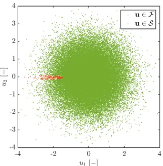
Figure 1 illustrates the topology of the limit state function of Adjiman’s
function in the standard normal spaceU. Herein,u1 and u2 respectively
cor-respond to u1 =Tu(x1) and u2 =Tu(x2), with Tu :X 7→ U a transformation
operator mapping responses from physical to standard normal space. This
plot is generated by performing 5·104Monte-Carlo evaluations of the
analyt-ical function, with a threshold value of yth= 3.7. The red dots in this figure
indicate the samples laying in the failure domainF (i.e., I ≤0), whereas the
samples in the safe domain S (i.e., I >0) are indicated in green. As it may
Figure 1: Failure domain F and safe domain S in standard normal space for Adjiman’s
function
Figure 2 shows the estimated failure probability, as obtained using Monte
Carlo, Advanced Line Sampling and SubSet-∞, as a function of the threshold
value. First, it can be seen that the estimate of the failure probability as a
function of the threshold of y is approximately equal for Monte Carlo and
the SubSet methods, as long as the failure probability remains moderately
large (i.e., Pf > 10−3). However, the obtained results diverge significantly
when smaller failure probabilities are computed. Advanced Line Sampling
on the other hand provides in this case a better estimate for the smaller
failure probabilities, which is explained by the independence of Line Sampling
performance to the magnitude of the probability of failure [29].
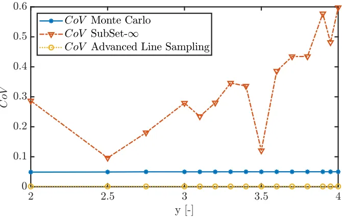
Figure 3 shows the CoV of the failure probabilities estimated by the
three methods. It can be noted that the variance on the failure probability
predictor that is obtained by Monte Carlo and Advanced Line Sampling is
up to a factor 5 smaller as compared to SubSet-∞. This is a direct result
Figure 2: Estimated failure probability and the coefficient of variance for different
thresh-old values y for Adjiman’s function
additional samples were generated until a specified CoV of 5% was reached,
whereas the SubSet method was heuristically tuned to minimize the CoV of
the prediction. Moreover, in the case of SubSet, the CoV measures up to
60% in the case of the smallest considered failure probabilities.
Figure 4 shows the computational efficiency in terms of necessary number
of samples to perform the probability of failure estimate. From this figure,
it is clear that SubSet-∞ is more efficient than Advanced Line Sampling,
which in its turn is more efficient than standard Monte Carlo simulation for
the estimation of the failure probability. This is particularly true when small
failure probabilities are considered. However, in that context it should be
noted that the variance of the Monte Carlo estimator is an order of magnitude
Figure 3: Estimated failure probability and the coefficient of variance for different
thresh-old values y for Adjiman’s function
the credibility of the estimate. The variance of Pf obtained via Advanced
Line Sampling is approximately equal to that of Monte Carlo, albeit at a
strongly reduced computational cost.
It should be noted that SubSet-∞, the most efficient technique, still
re-quires more than 2000 model evaluations, which is prohibitive when the
estimation of the failure probability of a structure using computationally
expensive computer models m() is considered.
As such, it can be concluded that although highly performing advanced
Monte Carlo methods exist to date, the estimation of small failure
probabil-ities in highly non-linear models still can prove to be computationally very
demanding. Therefore, even using these advanced Monte Carlo methods,
impor-Figure 4: Number of necessary samples of the advanced Monte Carlo methods for different
threshold valuesy for Adjiman’s function
tance, as the training of such surrogate model typically requires less model
evaluations as compared to a direct application of the advanced Monte Carlo
methods for the estimation of a small probability of failure. As discussed in
section 2, this however imposes uncertainty on the prediction of the failure
probability as well.
3.2. Surrogate model based estimation
This section presents results of the effect of the selection of the
surro-gate modeling approach and corresponding training on the uncertainty that
is attributed to the prediction. Using the constructed surrogate models,
de-creasing levels of failure probability are estimated by performing Monte Carlo
sampling until the CoV of the predictor was less than 5%, analogously to the
method that was applied in section 3.1.
[image:21.612.113.502.124.315.2]constructed surrogate models is illustrated in figures 5 - 7. For the Kriging
models, the 2 · σ bounds are considered, which yield a 95.5% confidence
interval forPf. For the IPM the uncertainty in the bounds onPf is considered
as being less than when β = 1− 96. In other words the bounds on Pf
obtained from integrating over the bounds of the IPM must be expanded by
.
Figure 5 illustrates the performance of the regular Kriging surrogate
mod-eling approach. Specifically, the ±2·σ bounds are illustrated together with
the crisp (mean) estimate of the model for all considered training data sets.
Also the prediction of the failure probability using the analytic model is
il-lustrated. First, in case sufficient data are used for the training, the regular
Kriging is capable of providing a relatively accurate crisp estimate of the
failure probability, as long asPf >5·10−03. For smaller failure probabilities,
Kriging fails in all cases. Second, it can be noted that the Kriging prediction
is conservative in the sense that the ±2·σ alway encompass the true
fail-ure probability. However, the lower bound prediction fails in all cases when
y > 3.7. This is due to the difficulty of sampling small failure probabilities
with standard Monte Carlo with a limited sample set. Finally, when more
data are included in the training of the Kriging model, the ±2·σ bounds
on the prediction become tighter. This is a direct result of the conditioned
random field that underlies these predictions. When more points are located
throughout the model domain, the relative distance between training points
decreases, and as such also the variance of the predicted random variable.
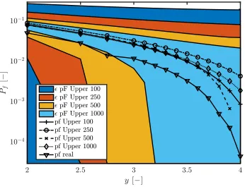
Figure 6 illustrates the performance of the interval predictor model in
pre-Figure 5: Performance of the Kriging surrogate models trained with different data sets in
predicting the failure probability of Adjiman’s function. For clarity, only the results of the
models trained with 100 and 1000 are shown.
diction of the upper limit of the failure probability ¯Pf are illustrated for all
data sets. Also the prediction of the failure probability using the analytic
model is illustrated. Only the upper bound of the IPM is illustrated for
visualization purposes, since this is the most relevant from an engineering
standpoint. First, it can be seen that except for y = 2 and y = 2.6, the
exact failure probability always lies inside the bounds of the upper bound
prediction of the IPM. Hence, the IPM always gives a safe estimation of the
[image:23.612.126.467.141.405.2]for the model trained with 1000 samples, the bounds inflate very quickly,
making the estimate very conservative. This behavior is more pronounced for
smaller data sets, since the confidence in the interval is proportional to the
size of the training data set. Finally, it can be noted that the upper bound
prediction of the set, without taking into account is more accurate than
the IPM that is trained with 1000 samples. This indicates over-training of
the polynomial basis, which is possibly aggravated by the iterative pruning
[image:24.612.123.469.324.589.2]of the polynomial basis as explained in section 2.2.
Figure 6: Performance of the IPM surrogate models trained with different data sets in
predicting the failure probability of Adjiman’s function.
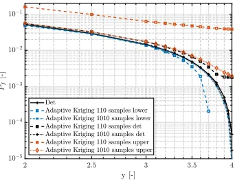
Specif-ically, the ±2·σ bounds are illustrated together with the crisp (mean)
es-timate of the model for all considered training data sets. Also the
predic-tion of the failure probability using the analytic model is illustrated. First,
the crisp estimate of the adaptive Kriging model is highly accurate for all
datasets, except for the model trained with 110 samples. Furthermore, when
Pf <2·10−04 the crisp accuracy degrades quickly. The±2·σ bounds on the
prediction are in all cases conservative w.r.t. the actual failure probability.
It can be noted that the prediction bounds of the adaptive Kriging model are
less over-conservative as compared to the regular Kriging model. This is a
direct result from the fact that the adaptive training procedure of the Kriging
model directs more training points towards the zone with a high probability
of failure. Therefore, given the same number of training points, the sampling
will be denser in the region of the input space where the extrema of the
function are locate, and as such, the variance of the Kriging estimator will
locally be lower in this region.
As such, the best performing method of the considered surrogate models
in terms of needed training data, accuracy and conservatism of the predicted
Pf is adaptive Kriging. This can be explained by the fact that the adaptive
Kriging model aims at optimizing the surrogate model performance in those
regions where extrema of the model are located. However, in other regions of
the model, the adaptive Kriging model generally is expected not to perform
well due to a lack of local training points. In general, the improved
per-formance of Adaptive Kriging when compared with Kriging should inspire
Figure 7: Performance of the Adaptive Kriging surrogate models trained with different
data sets in predicting the failure probability of Adjiman’s function. For clarity, only the
results of the models trained with 110 and 1010 are shown
the IPM is worst due to the comparatively high value of .
Finally, it can be seen that by using a surrogate model, computational
expenses for evaluating small failure probabilities can be decreased
drasti-cally. This statement is based on the argumentation that the application of
advanced Monte Carlo methods for the estimation of small failure
probabil-ities in conjunction with non-linear limit-state functions might prove to be
computationally very demanding when a full-scale numerical model is used
4. Conclusions
In case highly non-linear limit state functions occur in the estimation
of small failure probabilities, advanced Monte Carlo methods such as Line
Sampling or SubSet simulation may perform poorly or may still need a large
number of deterministic model evaluations to converge to a sufficiently small
coefficient of variance on the estimator. Less expensive surrogate models that
are calibrated in a supervised learning approach are therefore often used.
However, these surrogate model prediction introduce a further level of
un-certainty due to their approximative nature. This paper presents a study on
the robust estimation of small failure probabilities in strong non-linear
mod-els. Specifically, Kriging and Interval Predictor Models are employed since
they give an estimate of the uncertainty on the computed model response,
and hence, provide the analyst with a confidence interval on the prediction.
Since the intervals are used to model the uncertainty on the surrogate model
estimation superpose on the propagated variability stemming from the
ran-dom model parameters, the failure probability should be computed using a
probability box formulation of the model response. It is shown that this
problem reduces to computing two separate failure probabilities, using only
a single run of model evaluations. Therefore, instead of focusing on the crisp
estimate of the surrogate model to compute the probability of failure, it is
suggested to take the corresponding uncertainty into account. For practical
purposes, it is moreover even sufficient to consider the upper bound on the
failure probability prediction. Care should be taken however in the
construc-tion of the surrogate, as very conservative bounds on the estimate can occur
Acknowledgements
The Flemish research foundation is acknowledged for their support in the
research project G0C2218N, as well as for the post-doctoral grant 12P359N
of Matthias Faes.
References
[1] P. Koutsourelakis, H. Pradlwarter, G. Schu¨eller, Reliability of structures
in high dimensions, part i: algorithms and applications, Probabilistic
Engineering Mechanics 19 (4) (2004) 409–417.
[2] S.-K. Au, J. L. Beck, Estimation of small failure probabilities in high
dimensions by subset simulation, Probabilistic engineering mechanics
16 (4) (2001) 263–277.
[3] S.-K. Au, E. Patelli, Rare event simulation in finite-infinite dimensional
space, Reliability Engineering & System Safety 148 (2016) 67–77.
[4] S. K. Au, J. L. Beck, Subset simulation and its application to seismic risk
based on dynamic analysis, Journal of Engineering Mechanics 129 (8)
(2003) 901–917. doi:10.1061/(ASCE)0733-9399(2003)129:8(901).
[5] G. Schu¨eller, H. Pradlwarter, P. Koutsourelakis, A critical appraisal
of reliability estimation procedures for high dimensions, Probabilistic
engineering mechanics 19 (4) (2004) 463–474.
[6] H. Pradlwarter, M. Pellissetti, C. Schenk, G. Schu¨eller, A. Kreis,
estima-tion for aerospace structures, Computer Methods in Applied Mechanics
and Engineering 194 (12) (2005) 1597–1617.
[7] G. Schu¨eller, H. Pradlwarter, Benchmark study on reliability
estima-tion in higher dimensions of structural systems–an overview, Structural
Safety 29 (3) (2007) 167–182.
[8] B. Sudret, Global sensitivity analysis using polynomial chaos
expansions, Reliability Engineering & System Safety 93 (7)
(2008) 964 – 979, bayesian Networks in Dependability.
doi:https://doi.org/10.1016/j.ress.2007.04.002.
URLhttp://www.sciencedirect.com/science/article/pii/S0951832007001329
[9] M. Moustapha, J.-M. Bourinet, B. Guillaume, B. Sudret, Comparative
study of kriging and support vector regression for structural
engineer-ing applications, ASCE-ASME Journal of Risk and Uncertainty in
Engineering Systems, Part A: Civil Engineering 4 (2) (2018) 04018005.
arXiv:https://ascelibrary.org/doi/pdf/10.1061/AJRUA6.0000950,
doi:10.1061/AJRUA6.0000950.
URL https://ascelibrary.org/doi/abs/10.1061/AJRUA6.0000950
[10] M. Broggi, M. Faes, E. Patelli, Y. Govers, D. Moens, M. Beer,
Comparison of bayesian and interval uncertainty quantification:
Ap-plication to the airmod test structure, in: 2017 IEEE
Sympo-sium Series on Computational Intelligence (SSCI), 2017, pp. 1–8.
doi:10.1109/SSCI.2017.8280882.
quantifica-tion with kriging, in: 53rd AIAA/ASME/ASCE/AHS/ASC Structures,
Structural Dynamics and Materials Conference 20th AIAA/ASME/AHS
Adaptive Structures Conference 14th AIAA, 2012, p. 1853.
[12] D. G. Krige, A statistical approach to some basic mine valuation
prob-lems on the witwatersrand, Journal of the Southern African Institute of
Mining and Metallurgy 52 (6) (1951) 119–139.
[13] S. N. Lophaven, H. B. Nielsen, J. Søndergaard, Dace-a matlab kriging
toolbox, version 2.0, Tech. rep. (2002).
[14] R. Schobi, B. Sudret, J. Wiart, Polynomial-chaos-based kriging,
Inter-national Journal for Uncertainty Quantification 5 (2).
[15] M. De Munck, D. Moens, W. Desmet, D. Vandepitte, An efficient
re-sponse surface based optimisation method for non-deterministic
har-monic and transient dynamic analysis, Computer Modeling in
Engineer-ing and Sciences (CMES) 47 (2) (2009) 119.
[16] M. C. Campi, G. Calafiore, S. Garatti, Interval predictor models:
Iden-tification and reliability, Automatica 45 (2) (2009) 382–392.
[17] L. G. Crespo, D. P. Giesy, S. P. Kenny, Interval predictor models with
a formal characterization of uncertainty and reliability, in: Decision and
Control (CDC), 2014 IEEE 53rd Annual Conference on, IEEE, 2014,
pp. 5991–5996.
[18] L. G. Crespo, S. P. Kenny, D. P. Giesy, Interval predictor models with
a linear parameter dependency, Journal of Verification, Validation and
[19] L. G. Crespo, S. P. Kenny, D. P. Giesy, Staircase predictor models for
reliability and risk analysis, Structural Safety 75 (2018) 35–44.
[20] W. Verhaeghe, W. Desmet, D. Vandepitte, D. Moens, Interval fields to
represent uncertainty on the output side of a static FE analysis,
Com-puter Methods in Applied Mechanics and Engineering 260 (0) (2013)
50–62. doi:10.1016/j.cma.2013.03.021.
[21] M. Faes, J. Cerneels, D. Vandepitte, D. Moens, Identification and
quan-tification of multivariate interval uncertainty in finite element models,
Computer Methods in Applied Mechanics and Engineering 315 (2017)
896–920. doi:10.1016/j.cma.2016.11.023.
[22] M. Faes, D. Moens, Identification and quantification of spatial interval
uncertainty in numerical models, Computers and Structures 192 (2017)
16–33. doi:10.1016/j.compstruc.2017.07.006.
[23] X. Liu, L. Yin, L. Hu, Z. Zhang, An efficient reliability analysis
ap-proach for structure based on probability and probability box models,
Structural and Multidisciplinary Optimization 56 (1) (2017) 167–181.
[24] E. Patelli, M. Broggi, S. Tolo, J. Sadeghi, Cossan software: A
multidis-ciplinary and collaborative software for uncertainty quantification, in:
Proceedings of the 2nd ECCOMAS thematic conference on uncertainty
quantification in computational sciences and engineering, UNCECOMP,
2017.
[25] H. Zhang, R. L. Mullen, R. L. Muhanna, Interval monte carlo methods
[26] C. Jiang, W. Li, X. Han, L. Liu, P. Le, Structural reliability analysis
based on random distributions with interval parameters, Computers &
Structures 89 (23) (2011) 2292–2302.
[27] E. Patelli, H. M. Panayirci, M. Broggi, B. Goller, P. Beaurepaire, H. J.
Pradlwarter, G. I. Schu¨eller, General purpose software for efficient
un-certainty management of large finite element models, Finite elements in
analysis and design 51 (2012) 31–48.
[28] M. de Angelis, E. Patelli, M. Beer, Advanced line sampling for efficient
robust reliability analysis, Structural safety 52 (2015) 170–182.
[29] M. De Angelis, E. Patelli, M. Beer, An efficient strategy for
comput-ing interval expectations of risk, Safety, Reliability, Risk and Life-Cycle