Cumulative Prospect Theory and Deferred Annuities

City, University of London Institutional Repository

Citation

:

This is the accepted version of the paper.

This version of the publication may differ from the final published

version.

Permanent repository link:

Link to published version

:

Copyright and reuse:

City Research Online aims to make research

outputs of City, University of London available to a wider audience.

Copyright and Moral Rights remain with the author(s) and/or copyright

holders. URLs from City Research Online may be freely distributed and

linked to.

City Research Online: http://openaccess.city.ac.uk/ [email protected]

Cumulative prospect theory and deferred

annuities

ABSTRACT

Purpose– Although it has been proved theoretically that annuities can provide optimal consumption during one’s retirement period, retirees’ reluctance to purchase annuities is a long-standing puzzle. The purpose of this paper is to use behavioral model to analyse the low demand for immediate annuities.

Design/methodology/approach– The authors employ Cumulative Prospect Theory (CPT), which contains both loss aversion and probability transformations, to analyse the annuity puzzle.

Findings– The authors show that Cumulative Prospect Theory (CPT) can explain the unattractiveness of immediate annuities. It also shows that retirees would be willing to buy a long-term deferred annuity at retirement. By considering each component from CPT in turn, the loss aversion is found to be the major reason that stops people from buying an annuity; while the survival rate transformation is an important factor affecting the decision of when to receive annuity incomes.

Originality/value– This paper identifies CPT as one of the reasons for the low demand of immediate annuities. It further suggests that long-term deferred annuities could overcome behavioral obstacles and become popular among retirees.

1 Introduction

During the past few decades, traditional defined benefit (DB) pension plans have been losing their dominance in private sector pension systems in many countries; there has been a steady shift from DB pension plans towards defined contribution (DC) pension plans. Between 1980 and 2013, the number of participants in US private sector DC plans had increased more than fourfold from 20 million to 92.5 million; while participants in US private sector DB plans only increased from 38 million to 39 million (US Department of Labor, 2013). A more extreme shift can be observed in the United Kingdom (UK)

where active membership of DC pension scheme increased from 0.9 million in 2007 to

3.2 million in 2014; while that of DB pension scheme decreased from 2.7 million to 1.6

million during the same period (ONS, 2014). It is widely anticipated that pensioners will rely heavily on the DC pension plans in the future.

out a periodic income for as long as the annuitant is alive, in exchange for a premium charge. However, a low volume of premiums of voluntary annuities has been found in many international markets. Before a significant pension reform in 2011, in the UK, there used to be two markets: a compulsory one and a voluntary one. According to the sales figure reported in Cannon and Tonks (2011), the total compulsory annuity premium

income grew to around£11.5 billion in 2010, while the voluntary annuity premium only

amounted to£72 million.

The disparity between the theoretical optimal choice and the consumers’ real prefer-ences leads to the “annuity puzzle”. Since Yaari (1965) first demonstrated the benefit of annuitisation in a life cycle model with uncertain lifetime, the subsequent literature on annuities has provided various reasons to explain the low demand for annuities. Major reasons include the mortality risk-sharing among family members (Brown and Poterba, 2000), the existence of provision through social security and DB pension scheme mem-bership (Dushi and Webb, 2004) and the possibility of health care expenditure shocks at an old age (Davidoff, 2009).

While most conclusions are based on the assumptions that retirees are rational utility maximisers with risk-averse preferences, some recent studies have moved beyond the fully rational paradigm and proposed many behavioural factors that could play important roles in determining how retirees spend their retirement savings. For example, the decision to annuitise depends on the way in which the available choices are presented (Framing Effect). It also depends on the level of financial education or the level of understanding about annuities. In this paper, we seek to explain the unattractiveness of annuities in the light of behavioural finance and we focus on the impact of Cumulative Prospect Theory (CPT) which addresses flaws in the expected utility hypothesis and risk aversion. This theory was initially proposed by Tversky and Kahneman (1992) to describe how individuals make choices involving risky outcomes. It states that investors are loss averse rather than risk averse and a certain transformation is performed in evaluating probabilities. Using descriptive models for CPT, many authors have explained economic anomalies that cannot be explained by rational models. For example, Benartzi and Thaler (1995) and Barberis et al. (2001) apply CPT in the explanation of the equity premium puzzle. Kaluszkaa and Krzeszowiec (2012) use CPT as a method to price insurance contracts.

towards receiving annuity incomes at a later stage. (iii) By conducting an elasticity analysis we conclude that loss aversion is the most influential factor on the decision to purchase immediate annuities while the probability transformation determines the decision to purchase deferred annuities.

This article is organized as follows. In the next section, we provides a detailed introduction of CPT: the value function and the probability transformation model. Then in Section 3, we measure the perceived value of an annuity using the CPT framework. In Section 4, we present the results of relative price difference of annuities. Section 5 presents an extensive sensitivity analysis. Finally, Section 6 concludes the results and comments on the limitations of the analysis.

2 Introduction to Cumulative Prospect Theory (CPT)

CPT is a behavioural model that aims to capture decision making under risk and un-certainty. It states that the overall value of a risky investment is determined by three components: a reference point, a value function and a set of decision weights.

Being different from the utility function in expected utility theory, the value function

(v(·)) in CPT has three new properties. Firstly, the value function is based on the distance

(y) between the investment outcome and a reference point, rather than the terminal

investment outcome in the utility function. In a risky investment, the initial outlay to enter the investment is often regarded as the reference point. Investors would not simply consider the investment outcome as the gain; instead, they will deduct the initial outlay from the investment outcome and their satisfaction gained from the investment is based on this. Secondly, while the utility function describes simply a concave picture,

the value function is concave above the reference point (v00(y)<0,y>0) and convex

below the reference point (v00(y)>0,y<0). This can be illustrated by an example: the

satisfaction increase between a win of£100 and a win of£200 appears to be greater

than the satisfaction increase between a win of£1100 and a win of£1200. Similarly,

the increment in sadness that people feel between a loss of£100 and a loss of £200

tends to be greater than the increment in sadness between a loss of£1100 and a loss of

£1200, unless the large loss would compel people to lower current living standard such

as moving to a less desirable neighborhood. In other words, the value function yields the property of diminishing sensitivity: the marginal value of both gains and losses generally diminish with the distance from the reference point. Furthermore, the value function captures an important characteristic of attitudes to changes in wealth: loss looms larger

than gains. Thus, most people are loss averse and the satisfaction gained from a£100

win cannot erase the sadness brought by a£100 loss. From an experiment conducted by

Kahneman and Tversky (1979), people feel it unattractive to enter the symmetric bet

of winningyor losingywith equal probability, which justifies the assumption that the

value function for losses is steeper than that for gains (v0(y)<v0(−y)fory≥0).

v(y) =

yα _ify≥0

−λ(−y)β _ify<0 (1)

Here,λ reflects the level of loss aversion andα andβ reflect diminishing sensitivity.

Tversky and Kahneman (1992) estimate thatλ =2.25 andα =β =0.88.

Whereas expected utility theory weights the utility at different states with the objec-tive true probability of each state, experiments conducted by Tversky and Kahneman (1992) show that for both positive and negative prospects, decision makers always overweight low probability events and underweight high probability events. Therefore CPT introduces a method to transform true probabilities to decision weights which reflect perceived possibilities.

CPT introduces a capacity function w to express decision makers’ opinions of

perceived likelihood of uncertain events. The capacity function w is a non-linear

transformation of the real probabilities p. Two natural boundaries are certainty (w(1) =

1) and impossibility (w(0) =0). The principle of diminishing sensitivity applies to the

capacity function as well; it means that the influence of a given change in probability diminishes with its deviation from the boundary. For instance, the change in probability of winning a prize from 0.9 to 1 has more impact than the change in probability of winning a prize from 0.6 to 0.7. Similarly, an increase of 0.1 in probability of winning a prize has more impact when the probability changes from 0 to 0.1 than when the

probability changes from 0.3 to 0.4. Therefore, the capacity function w is concave

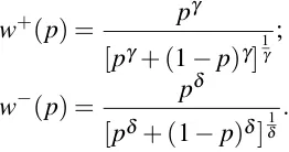
near 0 and convex near 1. In addition, the capacity function for positive and negative investment outcomes should be different because risk-seeking for small probability of gains is more pronounced than being risk-averse for small probability of losses. The capacity function is thus assumed to have the following form:

w+(p) = p

γ

[pγ_{+ (1−p)}γ_]

1

γ

;

w−(p) = p

δ

[pδ_{+ (1−p)}δ_]δ1

.

(2)

Figure 1 here

Based on experimental results in Tversky and Kahneman (1992),γ is estimated to

be 0.61 andδ to be 0.69. Figure 1 exhibits the shape of the capacity function. The

It reflects the point that risk aversion for gains is more pronounced for risk seeking for losses, for moderate and high probability events. Additionally, decision makers’ perceptions about probabilities coincide with the true probabilities around 0.35.

Let us define p_t as the probability of having an outcome y_t. We introduce the

following quantities:

π₁− =w−(p1),

π_t− =w−(p1+. . .+pt)−w−(p1+. . .+pt−1), 2≤t ≤k,

π_t+ =w+(pt+. . .+pT)−w+(pt+1+. . .+pT), k+1≤t≤T−1,

π_T+ =w+(pT).

(3)

where the risky outcomes have been ranked as:

y₁<y₂< . . . <y_k<0≤y_k+1< . . . <y_T.

The ultimate decision weight associated with an outcome is defined as the marginal

value of the respective event. The decision weightπ_t+, which corresponds to positive

investment outcomes, is the change in the value ofwbetween two events: “the outcome

is at least as good asy_t” and “the outcome is strictly better thany_t”. The decision weight

π_t−, which corresponds to negative investment outcomes, is the change in the value ofw

between the events: “the outcome is at least as bad asy_t” and “the outcome is strictly

worse thany_t”.

The value functions and the cumulative decision weights are combined to arrive at the overall value of a risky investment under CPT:

V(f−) =

k

∑

t=1

π_t−v(yt),

V(f+) =

T

∑

t=k+1

π_t+v(yt),

V(f) =V(f−) +V(f+).

(4)

Lettingπt=πt+ift≥k+1 andπt=πt− ift≤k, equation (4) can be reduced to:

V(f) =

T

∑

t=1

πtv(yt). (5)

3 Annuity valuations under CPT

of consumers’ attitudes towards annuities showed that virtually no consumer fully understands how an annuity product works; the least understood aspect of annuities is how risk sharing is performed so that insurers can offer a lifelong guaranteed income (Brown and Warshawsky, 2001). Because of this, consumers are more likely to focus on the risk of dying early, while overlooking the possibility that they may live well beyond their life expectancies and receive more than they have paid. They may also believe that the odds in the gamble tend to favor insurance companies. In another similar survey, the Society of Actuaries (2004) found that 49% of workers and 44% of retirees considered protecting against loss of value from a pension or annuity investment should they die earlier than expected as very important. Therefore, within this mental accounting framework, retirees tend to equate the lifetime annuity purchase with entering a gamble on their lives. CPT can be applied here to determine the overall value of annuities.

Viewing an annuity investment as a gamble, investors gain if total discounted annuity incomes exceed the annuity price; whereas investors lose if total discounted annuity income is below the annuity price. In other words, an annuitant gains if he outlives the life expectancy assumed in annuity pricing and loses if he dies before he collects as much income as he paid out. We assume that a retiree aged 65 purchases an immediate annuity

at an actuarially fair priceA, then the annuity investment outcome if the annuitant dies

aftertyears (at age 65+t) should be:

y_t =−A+

t

∑

i=1

Ψ 1

(1+r)i−1 (6)

whereΨrepresents the annual annuity income that is paid in advance and is assumed to

be 1 unit in our study;rrepresents the assumed constant interest rate;Ais the actuarially

fair price of an annuity that pays 1 unit per year in advance until the annuitant dies. No administrative fees or profit loadings are considered here.

The probability,p_t, that corresponds to each annuity outcomey_t, is the probability

that the 65-year-old retiree dies in exactlytyears, at age 65+t. With the inputy_t, we can

get the perceived value of the annuity investment according to equation (1). Furthermore,

we can transform probabilities pto decision weightsπbased on equations (2) and (3).

The overall value of the annuity can be calculated according to equation (5).

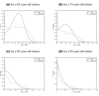
To reveal the impact of CPT probability transformations on mortality rates, Figure

2 shows the distorted probability π versus the original probability p when retirees

are at age 65, 75, 85 and 95. The results displayed are based on assumptions of an annual annuity payment of 1, an interest rate of 3% and an actuarially fair annuity price. It reflects that the ultimate decision weights will enhance the low probability of dying shortly after annuity purchase and the low probability of surviving a very long period after the annuity purchase. At the same time, it will decrease the probability corresponding to intermediate outcomes.

Figure 3 here

The transformation of the real probabilities will change people’s perceptions of their life expectancies. Figure 3 describes the differences between subjective complete life expectancies and real complete life expectancies for male individuals aged between 65 and 95. According to the figure, the distorted probability of dying at each age leads to the underestimation of life expectancies for young retirees and the overestimation of life expectancies for old retirees.

Following Hu and Scott (2007), we use the maximum acceptable price as a bench-mark measure to determine if an actuarially fairly priced annuity is desirable. The maximum acceptable price, also called the “reservation price”, is the highest price that a buyer is willing to pay for goods or a service. In the context of an annuity purchase, it is the price that would make an individual indifferent between purchasing an annuity and keeping the money in hand. According to equations (1) to (6), the overall value of an annuity can be regarded as a function of annuity price. The maximum acceptable annuity price is therefore the price that makes CPT value of an annuity equal to zero.

To facilitate our analysis, we calculate the ratioR, which is the relative difference

between reservation price and fair price.

R=Reservation Price−Actuarially f air price

Actuarially f air price

A positiveRmeans people would like to pay a higher-than-market price for an annuity

and thus the annuity is attractive. On the other hand, a negative R indicates

unattractive-ness. The modeling results in terms ofRcan also be interpreted as how much more or

less than market price one would be prepared to pay for an annuity.

4 Results

Due to the fact that no closed form solution forRexists, we solve it numerically. In our

analysis, we consider cumulative prospect theory with probability distortion (usingπ)

and without probability distortion (using p). For each one, we consider the situation

with loss aversion (λ >1) and without loss aversion (λ =1). Thus we can find out

how CPT influences people’s annuitisation decisions. In the following basic results, we have assumed that each parameter value in the CPT model is based on the values in

Tversky and Kahneman (1992). That meansλ =2.25 andα =β =0.88 for the value

function andγ =0.61 andδ =0.69 for the probability distortion function. In terms of

the annuity types, we are interested in both the immediate annuities that are purchased from age 65 to age 95 and the deferred annuities with deferred period from one year to thirty years (all purchased at age 65). We assume a constant interest rate of 3 percent.

The mortality rates are calculated from the recent standard mortality table “S2PML1”,

which contains the mortality experience of male pensioners of self-administered UK pension schemes for the period 2004 to 2011.

Figure 4 here

Figure 5 here

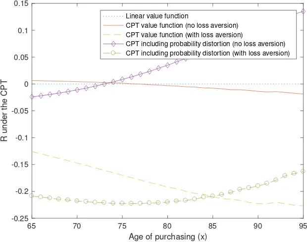
Figures 4 and 5 respectively show the trends in the R values for immediate and

deferred annuities under different versions of the CPT models. In the simplest model

of linear value function with no loss aversion and no probability transformation, R

remains 0 for both types of annuity. It reflects the fact that a risk-neutral individual who adopts a linear value function should be indifferent between purchasing an actuarially fairly priced annuity and keeping the money at hand. With the full CPT framework (CPT including probability distortion and with loss aversion), we notice that immediate annuities are generally not attractive for retirees between age 65 and age 95. Hence, CPT can be used as a behavioral explanation for people’s not buying immediate annuities. In addition, for a 65-year-old retiree, his/her preference for a deferred annuity is always increasing with the deferred period. In the following, we will analyse each component in the CPT framework.

Comparing the values ofRfor CPT models with loss aversion to those without loss

aversion, we notice that in both the immediate annuity case of Figure 4 and the deferred

annuity case of Figure 5,Rshifts downwards significantly once the loss aversion factor

is incorporated. This shifts the results in terms of the relative price difference from positive to negative for both immediate annuities and deferred annuities. Therefore, immediate annuities are not attractive for loss-averse individuals who are afraid of dying before reaching average life expectancies and deferred annuities are not attractive for loss-averse individuals who worry about dying within the deferred period. Hence, loss aversion is able to explain the low attractiveness of annuity products. Additionally, comparing the results for the CPT value function with loss aversion in Figure 4 with those

in Figure 5, the magnitude of the change inRis much smaller for immediate annuities

than for deferred annuities. It indicates the behavioural obstacle of loss aversion has greater impact on the choice of deferred annuities than immediate annuities. One may notice that the conclusion relies heavily on the assumed value for the loss aversion factor (which is 2.25); in the next section, we will discuss the stability of the results under a range of values of loss aversion.

In Figure 4 and Figure 5, we see the impact of probability distortion on immediate

annuities and deferred annuities respectively by comparing the values of R for the

“CPT value function (no loss aversion)” with those for the “CPT including probability distortion (no loss aversion)”. The probability distortion does not lead to the vertical

relation to the age of purchasing (x) or the deferred period (d). The probability distortion makes immediate annuities become more preferable for older retirees than younger

retirees asRis increasing smoothly with the age of purchase. Given the fact that more

elderly retirees have a smaller possibility of surviving, they overestimate the survival rate to a greater degree and would be prepared to pay a higher price for immediate annuity products. The same reasoning applies for deferred annuities. Retirees who follow CPT overestimate the low probability event of surviving for a long period to a greater degree and therefore a longer deferred period is much more preferred. Overall, overweighting of low probability events suggests that people buy annuities that provide income at an older age, or suggests that there should be a gap between the purchase date and the payment date.

Among all types of annuities discussed, a 30-year deferred annuity is predicted to be the most attractive. Since the chance of surviving from age 65 to age 95 is very

low at 0.068 (based on S2PML), the 30-year deferred annuities may be perceived as a

similar product to a lottery ticket. Cumulative Prospect Theory has been used to explain why individuals love buying classical lottery tickets which have negative expected outcome(Kahneman and Tversky, 1979).

5 Sensitivity analysis

In the above calculations, we have assumed that each parameter value is based on the values in Tversky and Kahneman (1992). Although the results may have biases because the annuity investment decision typically involves a much larger amount of money than the gambles used in Tversky and Kahneman’s psychological experiments, they still provide a good qualitative explanation for the attractiveness of different types of annuities. In this section, we conduct several sensitivity analyses to find out the relative attractiveness of annuities with regard to each parameter. The parameters we examine

are: loss aversion,λ, interest rate,r, the curvature of the capacity function,δ andγ, and

the probability of dying at exact age, p(by changing mortality tables).

5.1 Loss aversion sensitivity

The purpose of this sensitivity test is to discover whether retirees with different levels of loss aversion would like to annuitise their DC account balances. We increase the degree

of loss aversion gradually fromλ =1 (no loss aversion) toλ =5. Figure 6 displays the

shape ofRunder the CPT framework with regard to different annuity types and different

levels of loss aversion.

Figure 6 here

more loss averse, the losses arise from an annuity investment in the first few years will be perceived to be greater than the real values; then individuals would like to pay a lower price to enter an annuity contract. Additionally, comparing the two panels shows that immediate annuities are less attractive than deferred annuities. Immediate annuities can be attractive only when investors are not loss averse; on the contrary, a 30-year deferred annuity remains attractive even when investors’ loss aversion level increases to 2.25. As explained above, the popularity of the 30-year deferred annuities could be due to the

“lottery ticket effect”. Thirdly, the sensitivity ofRto the loss aversion degree is greater

for deferred annuities than for immediate annuities. It is mainly because, for a deferred annuity purchaser, the annuity investment does not deliver any income until after the deferred period. When compared with investing in an immediate annuity, a deferred annuity investor needs to wait longer for the overall investment outcome to become positive.

Many empirical studies have confirmed the importance of loss aversion and estimated the degree of loss aversion. According to Benartzi and Thaler (1995), when making a material economic decision, such as investing, it is appropriate to assume a loss aversion of 2. In the annuity decision analysis, we find that the 30-year deferred annuity is attractive if retirees’ loss aversion level is around 2.

5.2 Interest rate sensitivity

The interest rate is one of the most important factors to determine the price of an annuity and thus it may affect investment decisions. When the interest rate increases, both the annuity fair price and reservation price move downwards; it is therefore difficult to directly judge its influence on the overall attractiveness of annuities. In this section, we conduct an interest rate sensitivity analysis in order to explore whether retirees would be willing to convert their DC account balances into annuities when they are exposed to a range of interest rates from as low as 0.5 percent to as high as 8 percent.

Figure 7 here

Figure 7 shows the trend ofRfor the CPT framework for immediate annuities and

Regardless of how we change the interest rate, only the 30-year deferred annuity remains attractive among all annuity types. A major reason, as we have explained, is that deferred annuities with very long deferred periods are highly likely to be regarded as lottery tickets by retirees and thus may be attractive. Given the current low interest rate environment, immediate annuities are not an attractive purchase while the long term deferred annuities are predicted to be attractive.

5.3 Probability distortion sensitivity

In this section, we intend to discover the sensitivity of an annuity’s attractiveness to different levels of probability distortion. Both parameters in the capacity function (see

Equation (2)),δ andγ, which describe decision makers’ opinions of perceived likelihood

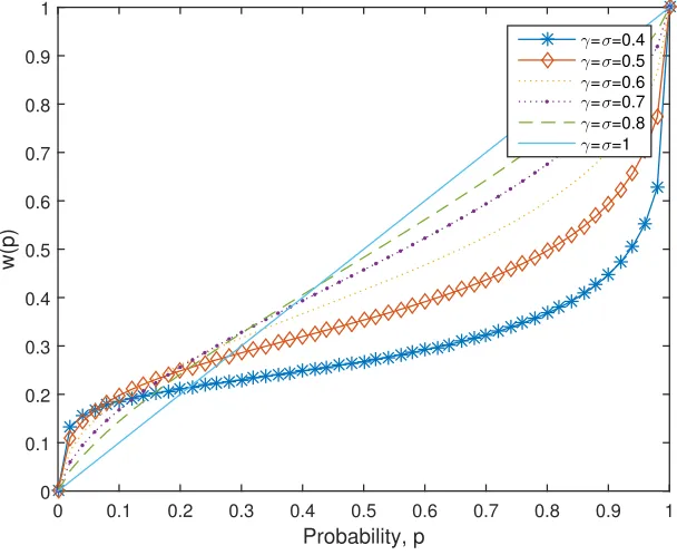
of uncertain events, are increased in steps of 0.1 from 0.4 to 1. Figure 8 shows the

capacity function of the real probabilities and we can see that, whenγ andδ are kept

low, there is a high degree of twist in the probability values and thus one would assign higher weights to extreme outcomes and lower weights to intermediate outcomes. When

bothγ andδ are 1, there is no probability distortion.

Figure 8 here

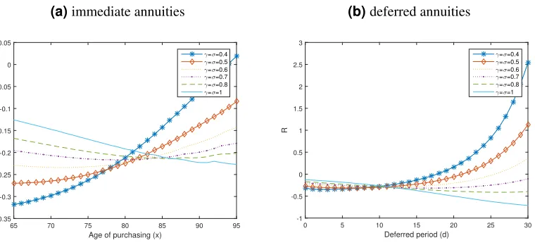
Figure 9 here

Figure 9 illustrates how the attractiveness of immediate annuities and deferred annuities is affected by weaker or stronger probability distortions. It clearly confirms our previous conclusion that a heavier distortion in probabilities would lead to choices of annuities that start paying at an older age. For immediate annuitants, it means buying an annuity at an older age; for deferred annuitants, it means buying one with a longer deferred period. On the other hand, if decision makers do not show any biases in probability estimation, the best annuity solution is an immediate annuity at age 65.

Many studies have examined the probability transformation and provided evidence on the level of distortion which we should apply to large gambles. In the experiments conducted by Tversky and Kahneman (1992), they allowed subjects to enter gambles with final payoffs as high as twice the median monthly family income and they estimated

the γ to be 0.61 and δ to be 0.69. Furthermore, Dodonova and Khoroshilov (2006)

provide evidence showing that smaller gambles normally have weaker probability distortion. Therefore, both sets of empirical evidence suggest a greater probability

distortion when we evaluate annuity decisions which involve large investments. Whenγ

andδ are around 0.4, annuities that are deferred for more than 20 years are attractive for

5.4 Mortality rates sensitivity

By changing the mortality assumptions, we can compare the attractiveness of annuities among different groups of people. In this section, we consider six different mortality

groups2. Our baseline results are based on S2PML, the mortality experience of male

pensioners of UK self-administered pension schemes for the period 2004 to 2011. S2PFL is the mortality experience of female pensioners for the same period. SPML03 captures the male pensioners’ mortality experience for a different period of time: 2000-2006. Additionally, to discover whether one’s pension amount would affect the decision to annuitise, the whole population dataset is divided into three subsets: L, S2PMA-M and S2PS2PMA-MA-H. S2PS2PMA-MA investigates the male pensioners’ mortality experience during 2004 and 2011 by considering the amount of pension. “Light” in S2PMA-L means that the benefit amount exceeds a specified amount and hence retirees in this group have relatively light mortality rates; “Heavy” in S2PMA-H means the benefit amount is lower than a specified amount and retirees in this group have relatively high mortality rates; “Medium” in S2PMA-M describes the mortality rate when the pension amount is intermediate.

Figure 10 here

Figure 10 shows the differences in mortality rates q_x3, the probability of death at

age x, among the six groups of people that make up the populations for these standard life tables. The improvement in mortality rates over time can be identified since male pensioners during an earlier period 2000-2006 have the highest mortality rates. In contrast, pensioners with a high pension size and female pensioners, during the period 2004-2011, have the lowest mortality rates among the six groups. As a result, pensioners in SPML03 have the shortest remaining lifetime, while those in S2PFL and S2PMA-L are expected to live longer than other pensioners of the same age.

Figure 11 here

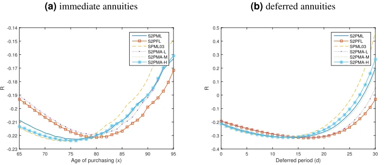
Figure 11 demonstrates the shape ofRunder these different mortality assumptions.

In the figure for immediate annuities, the shape ofRin relation to the age of purchase

shows that individuals with better health conditions prefer buying an immediate annuity earlier in retirement while those with worse health conditions tend to delay the purchase. This is reflected by comparing S2PFL vs. S2PML and S2PML vs. SPML03. Moreover,

comparing R values under S2PMA-L, S2PMA-M and S2PMA-H demonstrates that

retirees with high pension benefits are more likely to purchase immediate annuities early in retirement.

2_{The source for the mortality table SPML03 is the Continuous Mortality Investigation (2008); all other}

mortality tables come from Continuous Mortality Investigation (2013)

In terms of the deferred annuity, all groups find the 30-year deferred annuity the most attractive to buy among all of the deferred annuity products considered. Moreover, it is worth noticing that the 30-year deferred annuity is more popular among pensioners with higher mortality rates. This is because, for pensioners who have a lower possibility of surviving to age 95, a greater level of probability distortion is involved in the mental accounting process and the 30-year deferred annuity becomes more valuable to them. As a result, male pensioners during the period 2000-2006 would be the most interested in long-term deferred annuities while female pensioners and high-income pensioners show the least interest.

5.5 A comparison of parameter sensitivity

In order to measure the responsiveness of the Relative Price Difference to the change

in each parameter, we calculate the elasticity of the Relative Price Difference,E_R. It

addresses the percentage change in the Relative Price Difference for a given percentage change in the parameter value and the formula is as follows:

ER=

Percentage change inR

Percentage change in parameter value =

4R Raverage

4parameter parameteraverage

(7)

In Equation (7),4Rstands for the absolute change in R and4parameterstands

for the absolute change in the considered parameter values. Raverage stands for the

absolute value of average of R under different parameter values andparameter_averageis

the absolute value of the average of chosen parameter values. As the average value is used to calculate the percentage change, the elasticity of the Relative Price Difference

can be regarded as a point mid-way among all of theRresults. After we calculateE_R

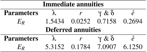
for all ages of immediate annuity purchases and for all deferred periods of deferred annuities, we average the results and obtain the elasticity of the Relative Price Difference for immediate annuities and for deferred annuities respectively. The results are presented in Table 1. Please note that we use life expectancy at the age of annuity purchase as an index for each mortality table.

Table 1 here

IfE_Ris greater than 1, the Relative Price Difference changes proportionately more

than the parameter value changes. If E_R is less than 1, the Relative Price Difference

changes proportionately less than the parameter value changes, implying a less sensitive parameter. Based on the results in Table 1, the following conclusions can be drawn. First, loss aversion is a very sensitive factor for both immediate and deferred annuities. It confirms our finding in the previous sections that loss aversion could be the major reason for the low valuation of annuity products. Second, an interesting finding is that

deferred annuities, but a small impact on that of immediate annuities. It indicates that people who have different levels of mortality rates transformation would have similar preferences for immediate annuities but distinct preferences for deferred annuities. Similarly, the deferred annuity have greater sensitivity to mortality parameters than immediate annuities, which is as we would expect. Finally, the elasticity of the Relative Price Difference for deferred annuities is in general much higher than that for immediate annuities, which justifies our previous conclusion that CPT has a greater impact on deferred annuities than immediate annuities.

6 Conclusions

Classical expected utility maximization theory suggests that annuities provide optimal consumption during a retiree’s retirement period, and hence it does not explain why the majority of retirees do not voluntarily convert their DC pension account balances into annuities. In this paper, we move beyond the rational paradigm that is assumed by the expected utility theory, in an attempt to discover if behavioral factors may be able to explain the way that people spend their retirement funds. We have applied cumulative prospect theory (CPT) to calculate the overall perceived value of annuities, from which we obtain the maximum price that individuals would like to pay for an annuity. By comparing this with the annuity price, we are able to conclude whether annuities in the market are attractive. We have also conducted several sensitivity analyses to study the relative attractiveness of annuities with regard to each parameter in the CPT model.

Our work is an extension of the paper by Hu and Scott (2007), who show that CPT is one of the behavioural factors that prevent people from buying an annuity. After confirming their conclusions, we have the following additional findings under CPT assumptions. First, immediate annuities are in general not attractive for retirees aged from 65 to 95; deferred annuities with a longer deferred period are more preferable. Second, loss aversion is the major reason for not purchasing annuities; and distortions in probability shift preferences towards an annuity that starts paying at an older age. Third, loss aversion is the most influential factor for the purchase decision of immediate annuities; and the mortality rate transformation determines the decision to purchase deferred annuities.

Based on our findings, some recommendations can be drawn for life insurance companies to improve the demand for annuities. One recommendation is the launch of long-term deferred annuities, which seem to have many competitive advantages. Firstly, making an early purchase decision would give a lower price. Taking a 30-year deferred

annuity as an example, the price is only 0.64% of a comparable immediate annuity

aroused intensive discussion in the literature as a retirement solution (Milevsky, 2005; Scott et al., 2011).

Another recommendation is to introduce some additional product features in existing products to attract loss averse customers. Our research indicates that, the major reason for low demand is that individuals are afraid of making a loss from an annuity investment. It can be improved by providing a guaranteed period of payments that does not depend on the survival of annuitants, which is already a common feature in the annuity markets. In terms of deferred annuities, this could be a return of a certain percentage of premiums if annuitants die within a certain number of years. Of course, these additional features would make annuities more expensive; however, they also reduce the possible high losses and could make it more attractive for loss averse customers.

While we predict customer behaviors and recommend the design of possibly more attractive annuity products, our study has one limitation. The values of parameters in the CPT model are based on the work in Tversky and Kahneman (1992). Their experimental design involves gambles rather than annuity purchases. Therefore the results presented here are not precise quantitative predictions, but can only provide qualitative explanations of the relative attractiveness of various types of annuities.

REFERENCES

Barberis, N., Huang, M., and Santos, T. (2001). Prospect theory and asset prices. The

Quarterly Journal of Economics, 116(1):1–53.

Benartzi, S. and Thaler, R. H. (1995). Myopic loss aversion and the equity premium

puzzle. The Quarterly Journal of Economics, 110(1):73–92.

Brown, J. R. and Poterba, J. M. (2000). Joint life annuities and annuity demand by

married couples. Journal of Risk and Insurance, 67(4):527–553.

Brown, J. R. and Warshawsky, M. J. (2001). Longevity-insured retirement distributions from pension plans: Market and regulatory issues. NBER Working Paper 8064, National bureau of economic research.

Cannon, E. and Tonks, I. (2011). Annuity markets: Welfare, money’s worth and policy implications. Netspar Panel Papers 24, Netspar.

Continuous Mortality Investigation (2008). CMI working paper 32. Research and resources, Institute and Faculty of Actuaries.

Continuous Mortality Investigation (2013). Proposed “S2” tables. Research and re-sources, Institute and Faculty of Actuaries.

Davidoff, T. (2009). Housing, health, and annuities. Journal of Risk and Insurance,

76(1):31–52.

Dodonova, A. and Khoroshilov, Y. (2006). Prospect theory and small payoffs: An

experimental study. Atlantic Economic Journal, 34(4):503–504.

Dushi, I. and Webb, A. (2004). Household annuitization decisions: Simulations and

Hu, W. and Scott, J. S. (2007). Behavioral obstacles in the annuity market. Financial

Analysts Journal, 63(6):71–82.

Kahneman, D. and Tversky, A. (1979). Prospect theory: An analysis of decision under

risk. Econometrica, 47(2):263–292.

Kaluszkaa, M. and Krzeszowiec, M. (2012). Pricing insurance contracts under

cumula-tive prospect theory. Insurance: Mathematics and Economics, 50(1):159–166.

Milevsky, M. A. (2005). Real longevity insurance with a deductible: Introduction

to advanced-life delayed annuities (ALDA). North American Actuarial Journal,

9(4):109–122.

ONS (2014). Occupational pension schemes survey: 2014. Statistical bulletin, Office for National Statistics.

Scott, J. S., Watson, J. G., and Hu, W. (2011). What makes a better annuity? Journal of

Risk and Insurance, 78(1):213–244.

Society of Actuaries (2004). Retirement plan preferences survey report of findings. Post retirement needs and risks, Society of Actuaries.

Tversky, A. and Kahneman, D. (1992). Advances in prospect theory: Cumulative

representation of uncertainty. Journal of Risk and Uncertainty, 5(4):297–323.

US Department of Labor (2013). Private pension plan bulletin historical tables and graphs, 1975-2013. Employee benefits security administration, US Department of Labor.

Yaari, M. E. (1965). Uncertain lifetime, life insurance, and the theory of the consumer.

Figure 1.CPT capacity functionw(p)

Probability, p

0 0.1 0.2 0.3 0.4 0.5 0.6 0.7 0.8 0.9 1

w(p)

0 0.1 0.2 0.3 0.4 0.5 0.6 0.7 0.8 0.9 1

w+(p) w-(p) p

Table 1. Elasticity of the Relative Price Difference (ER)

Immediate annuities

Parameters λ r γ &δ e˚

E_R 1.5434 0.0252 0.7158 0.2694

Deferred annuities

Parameters λ r γ &δ e˚

E_R 5.3152 0.1784 7.0907 6.1250

Figure 2.Probability of dying at different ages

(a)for a 65-year-old retiree

65 70 75 80 85 90 95 100 105 110 115 120

Age at death

0 0.005 0.01 0.015 0.02 0.025 0.03 0.035 0.04 0.045 0.05 Probability Real Subjective

(b)for a 75-year-old retiree

75 80 85 90 95 100 105 110 115 120

Age at death

0 0.01 0.02 0.03 0.04 0.05 0.06 0.07 0.08 0.09 0.1 Probability Real Subjective

(c)for a 85-year-old retiree

85 90 95 100 105 110 115 120

Age at death

0 0.02 0.04 0.06 0.08 0.1 0.12 0.14 0.16 0.18 Probability Real Subjective

(d)for a 95-year-old retiree

95 100 105 110 115 120

Age at death

Figure 3. Complete life expectancies under the impact of CPT probability transformations

65 70 75 80 85 90 95

Age

2 4 6 8 10 12 14 16 18 20

Complete life expectancies

Real complete life expectancies Complete life expectancies under CPT

Figure 4. The Relative Price Difference (R) under CPT for immediate annuities

65 70 75 80 85 90 95

Age of purchasing (x) -0.25

-0.2 -0.15 -0.1 -0.05 0 0.05 0.1 0.15

R under the CPT

Linear value function

CPT value function (no loss aversion) CPT value function (with loss aversion)

Figure 5. The Relative Price Difference (R) under CPT for deferred annuities

0 5 10 15 20 25 30

Deferred period (d)

-1 -0.5 0 0.5 1 1.5 2

R under the CPT

Linear value function

CPT value function (no loss aversion) CPT value function (with loss aversion)

CPT including probability distortion (no loss aversion) CPT including probability distortion (with loss aversion)

Figure 6. The sensitivity of the loss aversion factor on the Relative Price Difference

(R) of annuities

(a)immediate annuities

Age of purchasing (x)

65 70 75 80 85 90 95

R

-0.5 -0.4 -0.3 -0.2 -0.1 0 0.1 0.2

λ=1

λ=1.5

λ=2

λ=2.25

λ=3

λ=5

(b)deferred annuities

Deferred period (d)

0 5 10 15 20 25 30

R

-1 -0.5 0 0.5 1 1.5 2

λ=1

λ=1.5

λ=2

λ=2.25

λ=3

Figure 7. The sensitivity of the interest rate on the Relative Price Difference (R) of annuities

(a)immediate annuities

Age of purchasing (x)

65 70 75 80 85 90 95

R -0.23 -0.22 -0.21 -0.2 -0.19 -0.18 -0.17 -0.16 -0.15 r=0.5% r=1% r=2% r=3% r=6% r=8%

(b)deferred annuities

Deferred period (d)

0 5 10 15 20 25 30

R -0.4 -0.3 -0.2 -0.1 0 0.1 0.2 0.3 r=0.5% r=1% r=2% r=3% r=6% r=8%

Figure 8. CPT capacity functionw(p)under different levels of probability distortion

Probability, p

0 0.1 0.2 0.3 0.4 0.5 0.6 0.7 0.8 0.9 1

w(p) 0 0.1 0.2 0.3 0.4 0.5 0.6 0.7 0.8 0.9 1

Figure 9. The sensitivity of the probability distortions on the Relative Price Difference

(R) of annuities

(a)immediate annuities

Age of purchasing (x)

65 70 75 80 85 90 95

R

-0.35 -0.3 -0.25 -0.2 -0.15 -0.1 -0.05 0 0.05

γ=σ=0.4

γ=σ=0.5

γ=σ=0.6

γ=σ=0.7

γ=σ=0.8

γ=σ=1

(b)deferred annuities

Deferred period (d)

0 5 10 15 20 25 30

R

-1 -0.5 0 0.5 1 1.5 2 2.5 3

γ=σ=0.4

γ=σ=0.5

γ=σ=0.6

γ=σ=0.7

γ=σ=0.8

Figure 10. A comparison of Mortality rates

Age

65 70 75 80 85 90 95 100 105 110 115 120

Logarithm of mortality rates

-5 -4.5 -4 -3.5 -3 -2.5 -2 -1.5 -1 -0.5 0

S2PML S2PFL SPML03 S2PMA-L S2PMA-M S2PMA-H

Notes:S2PML is the mortality experience of male pensioners of UK self-administered pension schemes for the period 2004 to 2011. S2PFL is the mortality experience of female pensioners for the period 2004 to 2011. SPML03 is the male pensioners’ mortality experience between 2000 and 2006. S2PMA-L, S2PMA-M and S2PMA-H represent male pensioners’ mortality experience during 2004 and 2011 by considering the size of pension savings: Light (L), Medium (M) and Heavy (H).

Figure 11.The sensitivity of the mortality rates on the Relative Price Difference (R) of annuities

(a)immediate annuities

Age of purchasing (x)

65 70 75 80 85 90 95

R

-0.23 -0.22 -0.21 -0.2 -0.19 -0.18 -0.17 -0.16 -0.15 -0.14

S2PML S2PFL SPML03 S2PMA-L S2PMA-M S2PMA-H

(b)deferred annuities

Deferred period (d)

0 5 10 15 20 25 30

R

-0.4 -0.3 -0.2 -0.1 0 0.1 0.2 0.3 0.4 0.5

S2PML S2PFL SPML03 S2PMA-L S2PMA-M S2PMA-H

Notes:S2PML is the mortality experience of male pensioners of UK self-administered pension schemes for the period 2004 to 2011. S2PFL is the mortality experience of female pensioners for the period 2004 to 2011. SPML03 is the male pensioners’ mortality experience between 2000 and 2006. S2PMA-L, S2PMA-M and S2PMA-H represent male pensioners’ mortality experience during 2004 and 2011 by considering the amount of pension: Light (L), Medium (M) and Heavy (H).