Analysis of a fractal ultrasonic transducer with a range of piezoelectric length scales

doi:10.1093/imamat/hxz006

Advance Access publication on 18 March 2019

Analysis of a fractal ultrasonic transducer with a range of piezoelectric

length scales

Ebrahem A. Algehyne and Anthony J. Mulholland∗

Department of Mathematics and Statistics, University of Strathclyde, 26 Richmond Street, Glasgow G1 1XH, UK

∗_{Corresponding author: anthony.mulholland@strath.ac.uk}

[Received on 19 December 2017; revised on 19 October 2018; accepted on 16 February 2019]

The transmission and reception sensitivities of most piezoelectric ultrasonic transducers are enhanced by their geometrical structures. This structure is normally a regular, periodic one with one principal length scale, which, due to the resonant nature of the devices, determines the central operating frequency. There is engineering interest in building wide-bandwidth devices, and so it follows that, in their design, resonators that have a range of length scales should be used. This paper describes a mathematical model of a fractal ultrasound transducer whose piezoelectric components span a range of length scales. There have been many previous studies of wave propagation in the Sierpinski gasket but this paper is the first to study its complement. This is a critically important mathematical development as the complement is formed from a broad distribution of triangle sizes, whereas the Sierpinski gasket is formed from triangles of equal size. Within this structure, the electrical and mechanical fields fluctuate in tune with the time-dependent displacement of these substructures. A new set of basis functions is developed that allow us to express this displacement as part of a finite element methodology. A renormalization approach is then used to develop a recursion scheme that analytically describes the key components from the discrete matrices that arise. Expressions for the transducer’s operational characteristics are then derived and analysed as a function of the driving frequency. It transpires that the fractal device has a significantly higher reception sensitivity (18 dB) and a significantly wider bandwidth (3 MHz) than an equivalent Euclidean (standard) device.

Keywords: fractal; ultrasound; transducer; finite element; renormalization; Sierpinski..

1. Introduction

Ultrasonic transducers are devices, which convert mechanical vibrations into electrical energy and conversely convert electrical energy into mechanical vibrations (Beyer & Letcher, 1969;Yang, 2006a,b). One of the main uses of ultrasonic transducers is the interrogation of optically opaque media, by emission of a mechanical wave (converted from electrical to mechanical energy) and the reception of the same wave (after navigating the medium of interest, the wave is converted back from mechanical to electrical energy). Piezoelectric ultrasonic transducers are the most common devices used to assess the structural integrity of safety critical components in, e.g. nuclear plants and are used extensively in medical imaging and therapies; there is therefore considerable interest in improving the design of these sensors and the global market for such devices is set to reach $6 billion by 2020 (iRAP, 2016). Piezoelectric ultrasonic transducers ordinarily use regular, periodic geometrical structures (Algehyne & Mulholland, 2015b; Alippi et al., 1993; Hayward, 1984; Mulholland, 2008; Orr et al., 2007).

© The Author(s) 2019. Published by Oxford University Press on behalf of the Institute of Mathematics and its Applications. This is an Open Access article distributed under the terms of the Creative Commons Attribution License (http://creativecommons.org/licenses/by/4.0/), which permits unrestricted reuse, distribution, and reproduction in any medium, provided the original work is properly cited.

Many biological species produce and receive ultrasound; however, generally speaking, their auditory physiology is highly complex in structure and often consists of resonators with a range of length scales (Algehyne & Mulholland, 2015a;Barlow et al., 2016;Chiselev et al., 2009;Eberl et al., 2000; de Espinosa et al., 2005; Miles & Hoy, 2006; Müller, 2004; Müller et al., 2006; Nadrowski et al., 2008;Robert & Göpfert, 2002). Due to this range of length scales, these natural transducers are able to operate over a wide range of frequencies (so-called broadband transducers). There is a strong motivation therefore to design a device whose structure spans a range of length scales. Fractal structures are a natural choice for such a device as they consist of a variety of length scales (Mulholland & Walker, 2011; Mulholland et al., 2011;Orr et al., 2008) and are therefore a prime candidate for investigation. Various authors have analysed wave propagation in fractal media (Abdulbake et al., 2003,2004;Barlow, 1998; Derfel et al., 2012;Falconer & Hu, 2001;Giona, 1996;Giona et al., 1996;Kigami, 2001;Strichartz, 1999) and in particular the Sierpinski gasket and its graph counterpart (Algehyne & Mulholland, 2015a, 2017). However, the Sierpinski gasket consists of a series of triangles that are all of the same size. To circumvent this disadvantage, this paper studies wave propagation in the complement of the Sierpinski gasket as this consists of triangles that span a broad range of length scales. This appears to be the first time wave propagation has been studied in this structure and opens up new possibilities for mathemati-cians who wish to study other types of field equations in a structure with multiple length scales. So this paper marks a significant departure from the previous works ofAlgehyne & Mulholland (2015a, 2017) as the introduction of piezoelectric resonators covering a broad range of length scales will produce a set of resonances across a range of frequencies and so provide the physical basis for a broadband device. This switch to the piezoelectric material being located in the complement of the Sierpinski gasket is the critical step in producing a marked improvement in the device performance. A new graph is derived here to describe this fractal and it transpires that it has the same adjacency matrix as its dual but now the edges are weighted. The physical model consists of the elastodynamic equations, Gauss’s law for the electrical activity and a coupling of the electrical and mechanical waves through the piezoelectric constitutive equations. To describe this model on the fractal graph, a new set of finite element basis functions are derived whose support consists of the edges of the graph. The discrete equations that arise require the inversion of a large (in the case of a pre-fractal) or infinite-dimensional (for the fractal case) matrix in order to describe the dynamics of the device. Fortunately, the self-similar structure of the graph enables a renormalization approach to be utilized, which leads to a new set of nonlinear recursion relations. These recursion relations can be used to study the pre-fractal structures (for a finite number of iterations) or the fractal structure (by studying their steady states). This paper then compares the key operational characteristics of the pre-fractal ultrasound transducer with that of a standard transducer design. It transpires that the fractal device has a significantly higher reception sensitivity (18 dB) and a significantly wider bandwidth (3 MHz) than an equivalent Euclidean (standard) device (Hayward, 1984).

1.1 The Sierpinski gasket dual

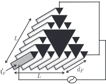
This transducer starts off as a piezoelectric crystal in a triangular structure, connected to three half-sized copies of itself (see Fig.1). The next generation (n=2) connects three half-sized copies of the smaller triangles to each of these triangles. Continuing in this way, the complement (or dual) of the standard Sierpinski gasket is produced. Using the complement (the black triangles in Fig.1) is vital as it has a range of triangle sizes, whereas the Sierpinski gasket is composed of triangles of the same size (the white triangles in Fig.1) for a given fractal generation level.

Fig. 1. The first few generations of the Sierpinski gasket (white triangles). The black triangles (the complement of the Sierpinski gasket) consist of piezoelectric material. The side length of the Sierpinski gasket is L for all generation levels.

1.2 Problem statement

Consider the vibrations of a Sierpinski gasket dual (denote this domain byΩ) made from a piezoelectric material (we will focus on PZT-5H) (Yang, 2006a) whose constitutive equations can be used to describe the interplay between the electrical and mechanical behaviour inΩ(Yang, 2006a,b)

T_ij = c_ijklS_kl−e_kijE_k, (1.1)

D_i = e_iklS_kl+ε_ikE_k, (1.2)

where the stress tensor is Tij, the stiffness tensor is cijkl, the strain tensor is Skl, the piezoelectric tensor is

ekij, the electric field vector is Ek, the electrical displacement tensor is Diand the permittivity tensor is

ε_ik(where the Einstein summation convention is adopted). The strain tensor describes the displacement gradients ui, jby Sij=(ui, j+uj,i)/2 and the electric field vector is related to the electric potentialφvia

E_i= −φ_,i. Governing the piezoelectric material’s dynamics is the following equation:

ρ_Tu¨_i=T_{ji, j}, (1.3)

subject to Gauss’ law

Di,i=0, (1.4)

where the density isρ_T and the ith component of displacement is ui. At this point, we will consider

the special case where there is only an out-of-plane displacement u = (0, 0, u3(x1, x2, t))(this is the dominant direction of displacement in engineering applications). The piezoelectric material is polarized in the x3 direction and the electrodes are arranged so that E = (E1(x1, x2), E2(x1, x2), 0). For the piezoelectric material, we choose PZT-5H (Auld, 1973). For this material (in Voigt notation), the various tensors above satisfy c₄₅=c₅₄ =0, c₄₄=c₅₅,ε_ik=0 apart fromε₁₁=ε₂₂andε₃₃, and e_ikl=0 apart from a small number of elements, which include e₁₁₃ =e₁₃₁=e₂₂₃=e₂₃₂(which in Voigt notation is e₂₄). Taking all of these restrictions on board then combining (1.1) with (1.3) gives

ρ_Tu¨₃=c₄₄(u_3,11+u_3,22)−e₂₄(E_1,1+E_2,2). (1.5)

Combining (1.2) and (1.4) gives

E_1,1+E_2,2 = −e24

ε₁₁(u3,11+u3,22). (1.6)

Combining (1.5) and (1.6) then gives

¨

u₃=c2_T∇2u₃, (1.7)

where∇2 _=∂2_/∂x2

1+∂2/∂x 2 2, cT =

cT₄₄/ρ_T is the shear wave velocity and cT₄₄ =c₄₄+e2₂₄/ε₁₁is the piezoelectrically stiffened shear modulus. We apply the boundary conditions of continuity of force and displacement on∂Ω as well as the initial conditions u3(x, 0) = ˙u3(x, 0) = 0. The challenge is to solve the above equations to calculate the dynamics of this device and to then use that to assess its performance as an ultrasonic transducer.

1.3 Galerkin discretization

Non-dimensionalizing via θ = cTt/h(n) and using the Laplace transform L : θ → q then gives

(dropping the subscript on u)

q2u¯ =h(n)2∇2u.¯ (1.8)

We will seek a weak solutionu¯ ∈ H1(Ω)where on the boundaryu¯ = ¯u_∂Ω ∈ H1(∂Ω). We multiply by a test function w ∈ H1_B(Ω), where H_B1(Ω):=w ∈ H1(Ω) : w = 0 on ∂Ω, integrate over the regionΩ and use Green’s first identity_Ωψ∇2φdv=_∂Ωψ(∇φ. n)dr−_Ω∇φ.∇ψdv, where n is the outward pointing unit normal of surface element dr. So, we seeku¯∈H1(Ω)such that

q2

Ω ¯

u w dx= −h(n)2

Ω

∇ ¯u .∇w dx,

where w ∈ H1_B(Ω). Following a standard Galerkin approach, we employ the finite-dimensional sub-spaces S_Sand S_B=S_S∩H1_B(Ω)rather than H1(Ω)and H_B1(Ω)and U_B∈S_Sto approximateu¯_∂Ω on the boundary∂Ω. The resulting discrete problem then requiresU¯ ∈S_Sto be found where

q2

Ω ¯

Uφ_jdx= −h(n)2

Ω

∇ ¯U .∇φ_jdx, j=1,. . ., N_n, (1.9)

where{φ₁,φ₂,. . .,φ_N

n}forms a basis of SB. The dynamics of each triangular component inΩ will be

described here by the dynamics of a single point at the centre of each of these components. Each of the basis functions will be centred on each of these points. Each triangular component inΩ is connected to some adjacent components and this connectivity will be captured here by joining these adjacent single points (or vertices) via edges to form a graph. The Sierpinski gasket graph of degree 3, SG, is the graph equivalent of the Sierpinski gasket (Schwalm & Schwalm, 1988). The dual graphSGis introduced in this paper and is constructed by a process that starts from the order n=1 design (which consists of four piezoelectric triangles) and assigns a vertex to the centre of each of the smaller triangles and, by connecting these vertices together with edges whose length is the side length of the larger triangle, the SG weighted graph at generation level n=1 is constructed (see Fig.2).

Fig. 2. The first few generations of the weighted Sierpinski gasket graph SG.

Fig. 3. The Sierpinski gasket dual lattice SG(3)at generation level n=1. Vertices B∈V_Ωo

n or V∂Ωnoin this level n=1 are the

input/output vertices, and vertices A∈V∂Ωnare fictitious vertices used to accommodate the boundary conditions.

The Sierpinski gasket has side length L units, which remain constant as the generation level n increases. The length of the smallest edge in the weighted graph SG(n)is h(n)=L/2nand the longest edge length that connects the three SG(n−1)graphs is h(1)=L/2. Then the overall diameter of the graph L(n)_SG=nL/2 and the total number of vertices is N_n = 3n_{. The vertex degree is 3 apart from the boundary vertices}

(input/output vertices), which have degree 2 and M_n=3(3n−1)/2 denotes the total number of edges at generation level n. The boundary vertices are used to interact with external loads (both electrical and mechanical) and fictitious vertices are introduced to cope with these interfacial boundary conditions. Denote byΩ_nthe set of points lying on the edges or vertices of the weighted graph SG(n)and denote the region’s boundary by∂Ω_n.

Definition 1.1 Denote the set of vertices inΩ_nas VΩn, the set of fictitious vertices as V∂Ωn (these

are vertices Nn+1, Nn+2 and Nn+3), the set of interior vertices as VΩo

n (so VΩno = VΩn \V∂Ωn)

and the set of input/output vertices as V∂Ωo

n (these are vertices 1, mn=(Nn+1)/2 and Nn) (see Figs3

and4). EΩn is the set of edges inΩn, the set of edges joining vertices in V∂Ωno to vertices in V∂Ωn is

Fig. 4. The Sierpinski gasket dual lattice SG(3)at generation level n =2. Vertices B and C ∈V_Ωo

n and vertices B ∈V∂Ωno.

Vertices A∈V∂Ωnare fictitious vertices used to accommodate the boundary conditions.

Fig. 5. Illustration of the identity E(_Ωp)o n = ¯E

(p−1) Ω_no₋₁.

denoted by E∂Ωn and EΩno is the set of the interior edges(EΩno = EΩn \E∂Ωn). Denote by E

(p) Ωo

n the

set of edges in EΩo

n of length h

(p) _{and byE}¯(p) Ωo

n three copies of E

(p) Ωo

n (the adjacency matrix for E¯Ωno is

a block diagonal matrix where each block is the adjacency matrix for EΩo n). E

(p) Ωn andE¯

(p)

Ωn are defined

similarly using the complete set of edges inΩ_n. Also,E¯∂Ωnis three copies of the boundary edges E∂Ωn.

Hence,E¯_Ω(p_n−₋1₁) =E(p)_Ωn if p<n,E¯(p_Ω−o1) n−1 =E

(p) Ωo

n for pn (Fig.5graphically illustrates this identity) and

E(p)_Ωo n =E

(p)

Ωnif p<n.

Letφ_i, i∈V_Ωn form a set of basis functions for the vertex displacements and let

¯

U=

Nn

i=1

U_iφ_i+

i∈V∂Ωn

U_Biφ_i. (1.10)

Hence, (1.9) becomes

A(n)_ji U_i=b(n)_j , (1.11)

where

A(n)_ji =q2H_ji(n)+h(n)2K(n)_ji , (1.12)

H_ji(n)=

Ωn

φ_jφ_idx, (1.13)

K_ji(n)=

Ωn

∇φ_j.∇φ_idx (1.14)

and

b(n)_j = −

i∈V∂Ωn ∂Ωn

q2φ_jφ_i+h(n)2∇φ_j.∇φ_i

dx

U_Bi, j∈V_∂Ωo

n. (1.15)

Lemma 1.1 The basis functionφ_jfor vertex j in the element (the edge) joining vertices j and k at fractal generation level n is given by

φ_jx, y, x_j, y_j, x_k, y_k, x_m, y_m, x_l, y_l

=(y−y_k)(x_m+x_l)−(x−x_k)(y_m+y_l)+2(xy_k−x_ky)+ x_jy−x_jy_k−xy_j+x_ky_j+xy_k−x_ky

(yj−yk)(xm+xl)−(xj−xk)(ym+yl)+2(xjyk−xkyj)

, (1.16)

where, for edges of length greater than h(n) and n2, the two other adjacent vertices to vertex j are l and m. For interior edges of length h(n)and n1, then vertex l is equal to vertex j and vertex m is the vertex that is connected to vertex j by the other edge of length h(n). For exterior edges—these will have length h(n)—then vertices l and m are also the two interior vertices adjacent to vertex j. Hence,

∇φ_j(x, y, x_j, y_j, x_k, y_k, x_m, y_m, x_l, y_l)

=

_−(y

j+ym+yl)+3yk

(y_j−y_k)(x_m+x_l)−(x_j−x_k)(y_m+y_l)+2(x_jy_k−x_ky_j), x_j+x_m+x_l−3x_k

(yj−yk)(xm+xl)−(xj−xk)(ym+yl)+2(xjyk−xkyj)

. (1.17)

Proof. The basis function is chosen to be linear having a value of one at vertex j and a value of zero at vertex k. So φ_j(n) is a straight line lying in a plane S_P containing the points P₂ = (x_k, y_k, 0)and P₁=(x_j, y_j, 1). To make this plane unique, a third point is required. When edge jk is longer than h(n),

then, to retain the symmetry inherent to the SG graph, this third point is chosen as the centroid of the triangle formed by the two other vertices(x_mand x_l)connected to vertex j and vertex j itself. When an interior edge jk has length h(n), then this third point is chosen as the centroid of the triangle formed by the two interior vertices that are connected to vertex j by edges of length h(n). So let P3be the point (x_j+x_m+x_l, y_j+y_m+y_l, 0)/3. The vectors a=−−→OP₁−−−→OP₃and b=−−→OP₂−−−→OP₃lie in this plane and so the equation of the plane is(a×b)·x=(a×b)·−−→OP₁. This is a scalar equation with the unknowns being the components of the vector x=(x, y, z). This equation is manipulated to make z the subject of the equation and the basis function in (1.16) is then given by the right-hand side of this equation. The

gradient then follows.

For a particular element of length h(p) lying between vertex j and vertex k, the isoparametric representation, given by

(x(s), y(s))=(x_k−x_j)s+x_j,(y_k−y_j)s+y_j (1.18)

is employed, where s∈[0, 1] anddx=h(p)ds.

2. Derivation of the matrix recursions

Using the basis function derived in Lemma1.1, it can be shown that the matrix H at fractal generation level n can be related to its counterpart at level n−1.

Lemma 2.1

ˆ

H_ji(n)= ¯ˆH_ji(n−1)+Υ(n)W_ji(n)+ϑ(n)P(n)_ji , j, i∈V_Ωo

n, (2.1)

whereH¯_ji(n−1)is a block diagonal matrix consisting of three blocks of matrix H_ji(n−1)for n2,H¯ˆ_ji(n−1)=

¯

H_ji(n−1)/h(n),Hˆ_ji(n)=H_ji(n)/h(n),Υ(n)=(2n−1−1)/3,ϑ(n)=2n−1/6, W_ji(n)=1_V(1) Ωn

(j)1_{0}(i−j)(where 1_{A}(a)is the indicator function, which equals 1 if a∈A and 0 otherwise) and P

(n) ji =1E(_Ω1)

n

(ji).

Proof. By using (1.13) and (1.18) for edge jk of length h(p), then

jk

H_cd(n,p)=

jk∈EΩn

φ_cφ_ddx=2n−ph(n) 1

0

φ_c(x(s), y(s)) φ_d(x(s), y(s))ds. (2.2)

From (1.16), the basis function at vertex j (which has coordinates(a, b)) along a typical edge jk ∈E(p)_Ω

n

where p<n is

φ_j(x, y)= 1 h(n)

(a−x)(3+2(1+p−n))−(b−y)√3+h(n)

(2.3)

and at vertex k (which has coordinates(a+2(n−p−1)h(n), b+2(n−p−1)√3h(n))) is

φ_k(x, y)= 1 h(n)

(a−x)(3+2p−n)−√3(b−y)1+2p−n. (2.4)

Substituting (1.18) into (2.3) and (2.4) gives

φ_j(x(s), y(s))=1−s

and

φ_k(x(s), y(s))=s. Now if(c=d=j)or(c=d=k)in (2.2), then

jk

H_jj(n,p) =2n−ph(n) 1

0

(1−s)2ds= 2

n−p

3 h

(n)₌jk

H_kk(n,p)

and if (c=j and d=k) or (c=k and d=j) in (2.2), then

jk

H(n,p)_jk =2n−ph(n) 1

0

(1−s)s ds=2

n−p

6 h

(n)₌jk

H(n,p)_kj .

A similar calculation can be conducted for the case p=n albeit the basis function calculation is slightly different and follows the prescription in the proof of Lemma 2. So (2.2) becomes, for jk∈E(p)_Ωn, n1 and pn

jk_H(n,p)

cd =2

n−p_h(n)

⎧ ⎪ ⎪ ⎪ ⎪ ⎨ ⎪ ⎪ ⎪ ⎪ ⎩ 1

3 if (c=d=j)or(c=d=k) 1

6 if (c=j and d=k)or(c=k and d=j), j=k 0 otherwise.

(2.5)

We now consider the basis functions at input/output vertices V∂Ωo

n and the integration of (2.2) in the

boundary edges jk∈E_∂Ωn. Equation (2.2) becomes

jk_H(n,n)

cd =h

(n)

⎧ ⎨ ⎩ 1

3 if (c=d=j∈V∂Ωo n)

0 otherwise.

(2.6)

The matrix H_cd(n)is assembled element by element (edge by edge) as follows:

H_cd(n)=

n

p₌1

jk∈E(_Ωp)

n

jk_H(n,p)

cd =

n

p₌2

jk∈E(_Ωp)

n

jk_H(n,p)

cd +

jk∈E(_Ω1_n) jk_H(n,1)

cd . (2.7)

The first term on the right-hand side of this equation can be written as

n

p=2

jk_∈E_Ω(p)

n

jk

H_cd(n,p) =

n₋1

p=2

jk_∈E(_Ωp)

n

jk

H_cd(n,p)+

jk∈E(_Ωn)

n

jk

H(n,n)_cd

= n−2

p=1

jk∈E_Ω(p +1)

n

jk_H(n,p+1)

cd +

jk∈E(_Ωn)

n

jk_H(n,n)

cd .

Since E_Ω(p)o n = ¯E

(p−1) Ωo

n−1, E

(p) Ωn = ¯E

(p−1)

Ωn−1, and E∂Ωn ⊆ ¯E∂Ωn−1 ⊆ ¯E

(n₋1)

Ωn−1 for 1 < p < n, then, E

(n) Ωn =

E(n)_Ωo

n ∪E∂Ωn = ¯E

(n−1)

Ω_no₋₁ ∪E∂Ωn =

¯

E(n_Ω−1)

n−1 \ ¯E∂Ωn−1

∪E_∂Ωn = ¯E(n_Ω−1)

n−1 \

¯

E_∂Ωn−1\E_∂Ωn

. Hence,

n

p=2

jk∈E(_Ωp)

n

jk

H_cd(n,p) =

n−2

p=1

jk∈ ¯E(_Ωp)

n−1

jk

H_cd(n,p+1)+

jk∈ ¯E_Ω(n−1)

n−1

jk

H(n,n)_cd −

jk∈ ¯E∂Ω_n−1\E∂Ωn

jk

H_cd(n,n)

= n−1

p=1

jk∈ ¯E(_Ωp)

n−1

jk_H(n,p+1)

cd −

jk∈ ¯E∂Ω_n−1\E∂Ωn

jk_H(n,n)

cd .

It can be shown thatjk_H(n,p+1)

cd =jkH

(n−1,p)

cd , and then from (2.6),

n

p=2

jk_∈E(_Ωp)

n

jk

H_cd(n,p) = ¯H_cd(n−1)−h

(n)

3 W

(n)

cd (2.8)

since inE¯_∂Ωn−1 \E_∂Ωn we have c = d in (2.5), andH¯_cd(n−1) is a block diagonal matrix of dimension Nn×Nnconsisting of three blocks given by H

(n−1)

cd of dimension Nn−1×Nn−1. Now the second term on the right-hand side of (2.7) can be written as

jk∈E(_Ω1)

n

jk

H(n,1)_cd =2n−1h(n) 1 6P (n) cd + 1 3W (n) cd .

Combining this with (2.8), then (2.7) becomes

ˆ

H_ji(n)= ¯ˆH(n_ji−1)+1 3(2

n−1_−1)W(n)

ji +

2n−1 6 P

(n) ji ,

whereH¯ˆ(n_ji−1)= ¯H_ji(n−1)/h(n)_andHˆ(n)

ji =H

(n)

ji /h(n).

A similar approach can be used to derive the matrix K_ji(n).

Lemma 2.2

ˆ

K_ji(n)= ¯ˆK_ji(n−1)+(n)W_ji(n)+χ(n)P(n)_ji , j, i∈V_Ωo

n, (2.9)

where K¯(n_ji−1) is a block diagonal matrix consisting of three blocks of matrix K_ji(n−1) for n 2,

¯ˆ

K_ji(n−1) = h(n)K¯_ji(n−1), Kˆ_ji(n) = h(n)K_ji(n), (n) = 2n−1(12 +24−2n +3(23−n)) −28 and χ(n) = 2n−1(12+23−2n+3(23−n)).

Proof. By using (1.14) and (1.18) for edge jk of length h(p), then

jk

K_cd(n,p)=

jk∈EΩn

∇φ_c.∇φ_ddx=2n−ph(n) 1

0

∇φ_c(x(s), y(s)).∇φ_d(x(s), y(s))ds. (2.10)

Equations (2.3) and (2.4) give for jk∈E(p)_Ωn where p<n

∇φ_j(x, y)= 1 h(n)

−3+2(1−n+p),√3

and

∇φ_k(x, y)= 1 h(n)

−3+2p−n,√31+2p−n.

Now if(c=d=j)or(c=d=k)in (2.10), then

jk

K_jj(n,p) = 2n−ph(n) 1

0 1 h(n)

−3+2(1−n+p),√3

. 1 h(n)

−3+2(1−n+p),√3

ds

= 2n−p

h(n)

12+2(2−2n+2p)+32(2−n+p)=jkK_kk(n,p)

and if (c=j and d=k) or (c=k and d=j) in (2.10), then

jk

K(n,p)_jk = 2n−ph(n) 1

0 1 h(n)

−3+2(1−n+p),√3

. 1 h(n)

−3+2p−n,√31+2p−nds

= 2n−p

h(n)

12+2(1−2n+2p)+32(2−n+p)=jkK(n,p)_kj .

Hence, for jk∈E(p)_Ω

n, n2 and p<n,

jk

K_cd(n,p)= 2

n−p

h(n)

⎧ ⎪ ⎪ ⎪ ⎪ ⎨ ⎪ ⎪ ⎪ ⎪ ⎩

12+2(2−2n+2p)+32(2−n+p) if (c=d=j)or(c=d=k)

12+2(1−2n+2p)+32(2−n+p) if (c=j and d=k)or(c=k and d=j)

0 otherwise.

(2.11)

A similar calculation can be undertaken for the case when jk∈E(n)_Ωo

n and p=n. It transpires that

jk_K(n,n)

cd = 1 h(n) ⎧ ⎪ ⎪ ⎪ ⎪ ⎨ ⎪ ⎪ ⎪ ⎪ ⎩

4 if (c=d=j)or(c=d=k)

2 if (c=j and d=k)or(c=k and d=j) 0 otherwise.

(2.12)

Similarly, for the boundary edges jk∈E∂Ωn, (2.10) becomes

jk_K(n,n)

cd = 1 h(n) ⎧ ⎨ ⎩

28 if (c=d=j∈V_∂Ωo n)

0 otherwise.

(2.13)

As before, the matrix K_cd(n)is assembled in an element by element (edge by edge) manner via

K_cd(n) =

n

p=1

jk∈E(_Ωp)

n

jk_K(n,p)

cd =

n

p=2

jk∈E(_Ωp)

n

jk_K(n,p)

cd +

jk∈E(_Ω1_n) jk_K(n,1)

cd . (2.14)

The first term on the right-hand side of this equation can be written as

n

p=2

jk∈E_Ω(p)_n jk

K_cd(n,p) =

n−1

p=2

jk∈E_Ω(p)_n jk

K_cd(n,p)+

jk∈E_Ω(n)

n

jk

K_cd(n,n)

= n−2

p=1

jk_∈E(_Ωp +1)

n

jk

K_cd(n,p+1)+

jk∈E(_Ωn)

n

jk

K_cd(n,n).

Since E(p)_Ω

n = ¯E

(p−1)

Ωn−1 for 1<p<n, and E

(n) Ωn =E

(n) Ωo

n ∪E∂Ωn = ¯E

(n−1)

Ω_no₋₁ ∪E∂Ωn =

¯

E(n_Ω−1)

n−1 \ ¯E∂Ωn−1

∪

E_∂Ωn = ¯E_Ω(n−1)

n−1 \

¯

E_∂Ωn−1 \E_∂Ωn

. Hence,

n

p=2

jk∈E(_Ωp_n) jk

K_cd(n,p) =

n−2

p ₌1

jk∈ ¯E(_Ωp)

n−1

jk

K_cd(n,p+1)+

jk∈ ¯E_Ω(n−1)

n−1

jk

K_cd(n,n)−

jk∈ ¯E∂Ω_n−1\E∂Ωn

jk

K_cd(n,n)

= n−1

p=1

jk∈ ¯E(_Ωp)

n−1

jk

K_cd(n,p+1)−

jk∈ ¯E∂Ωn−1\E∂Ωn

jk

K_cd(n,n).

It can be shown thatjkK_cd(n,p+1)=jkK_cd(n−1,p), and then from (2.13),

n

p=2

jk∈E(_Ωp)

n

jk_K(n,p)

cd = ¯K

(n−1)

cd −

28 h(n)W

(n)

cd (2.15)

by a similar argument to that in Lemma2.1. Examining the second term on the right-hand side of (2.14), and using (2.11) with p=1, gives

jk∈E(_Ω1)

n

jk_K(n,1)

cd =

2n−1 h(n)

12+23−2n+3(23−n)

P(n)_cd

+2n−1

h(n)

12+24−2n+3(23−n)

W_cd(n).

Combining this with (2.15), then (2.14) becomes

ˆ

K(n)_ji = ¯ˆK_ji(n−1)+(n)W_ji(n)+χ(n)P(n)_ji ,

where K¯ˆ_ji(n−1) = h(n)K¯_ji(n−1),Kˆ_ji(n) = h(n)K_ji(n),(n) = 2n−1(12+24−2n +3(23−n))−28 and χ(n) =

2n−1(12+23−2n+3(23−n)).

Theorem 2.1

ˆ

A(n)_ji = ¯ˆA(n_ji−1)+α(n)W_ji(n)+β(n)P(n)_ji , (2.16) whereA¯(n_ji−1)is a block diagonal matrix consisting of three blocks of matrix A_ji(n−1)for n2,A¯ˆ(n_ji−1)=

¯

A(n_ji−1)/h(n),α(n)=q2Υ(n)+ε(n)andβ(n)=q2ϑ(n)+χ(n). Proof. Combining (2.1) and (2.9) gives (1.12) as

ˆ

A(n)_ji = q2

¯ˆ

H_ji(n−1)+Υ(n)W_ji(n)+ϑ(n)P(n)_ji

+K¯ˆ_ji(n−1)+ε(n)W_ji(n)+χ(n)P(n)_ji

= q2H¯ˆ_ji(n−1)+ ¯ˆK_ji(n−1)+α(n)W_ji(n)+β(n)P(n)_ji .

As discussed in Algehyne & Mulholland(2015a), when redimensionalizing, we need to rescale the frequency by(c_T/h(n))−1. Hence,

ˆ

A(n)_ji = ¯ˆA(n_ji−1)+α(n)W_ji(n)+β(n)P(n)_ji ,

whereA¯ˆ(n_ji−1)=q2_H¯ˆ(n−1)

ji + ¯ˆK

(n₋1)

ji .

A similar treatment can be given to (1.15)

Lemma 2.3

b(n)_j =h(n)ηU_i1_E

∂Ωn(ji), j∈V∂Ωon, i∈V∂Ωn, (2.17)

whereη=4−q2_/6.

Proof. By using (1.15) and (1.18) for edge ji, then

b(n)_j = −

i∈V∂Ωn ji∈E∂Ωn

q2φ_jφ_i+h(n)2∇φ_j.∇φ_i

dx

U_Bi

= −h(n)

i∈V∂Ωn

1

0

q2φ_j(x(s), y(s)) φi(x(s), y(s))

+h(n)2∇φ_j(x(s), y(s)).∇φ_i(x(s), y(s))

ds

UBi, (2.18)

where j∈V_∂Ωo

n. From (1.16), the basis function at vertex j∈V∂Ωno (without loss of generality, we will

examine the vertex with coordinates(a, 0)) along a typical edge ji∈E_∂Ωnis

φ_j(x, y)= 1 h(n)

a+h(n)−x−3√3y

(2.19)

and at vertex i∈V∂Ωn(which has coordinates(a+h

(n)_{, 0)) is}

φ_i(x, y)= 1 h(n)

−a+x+√y 3

. (2.20)

Substituting (1.18) into (2.19) and (2.20) gives

φ_j(x(s), y(s))=1−s (2.21)

and

φ_i(x(s), y(s))=s. (2.22)

In addition, (2.19) and (2.20) give

∇φ_j(x(s), y(s))= 1 h(n)

−1,−3√3

(2.23)

and

∇φ_i(x(s), y(s))= 1 h(n)

1,+√1

3

. (2.24)

Substituting (2.21) to (2.24) into (2.18) gives

b(n)_j =h(n)

4−q 2

6

U_i j∈V_∂Ωo

n, i∈V∂Ωn and ji∈E∂Ωn.

2.1 Application of the mechanical boundary conditions

The transducer is electrically coupled to a power supply and is immersed in a mechanical load and appropriate electrical and mechanical boundary conditions can be applied (Algehyne & Mulholland, 2015a).

Theorem 2.2

Ui=G (n)

ji δ¯j, (2.25)

where

G(n)_ji =

ˆ

A(n)_ji − ˆB(n)_{ji −}1

(2.26)

represents the Green’s transfer matrix,Bˆ(n)_ji =diag{¯γ₁,. . .,γ¯_m

n,. . .,γ¯Nn},γ¯j=ηγj,δ¯j=ηδj,

γ_j= ⎧ ⎪ ⎪ ⎪ ⎪ ⎨ ⎪ ⎪ ⎪ ⎪ ⎩

1−qZ_B/Z_T−1, j=1

1−qZL/ZT

₋1

, j=mnor Nn

0 otherwise,

(2.27)

δ_j= ⎧ ⎪ ⎪ ⎪ ⎪ ⎨ ⎪ ⎪ ⎪ ⎪ ⎩

−γ₁ζQ/cT₄₄ξ, j=1

γ_mnζQ/cT₄₄ξ−2A_LqZ_L/Z_T, j=m_nor N_n

0 otherwise,

(2.28)

Z_Bis the mechanical impedance of the backing material, Z_L=μ_LA_r/c_Lis the mechanical impedance of the load, Z_T =cT₄₄A_r/c_T,ζ =e₂₄/ε₁₁, Q is the electrical charge,ξ =A_r/h(n), A_ris the cross-sectional area of the electrode, A_L is the amplitude of the incoming wave that is received by the transducer (in transmission mode A_Lis zero),μ_Lis the shear modulus of the load material and c_Lis its wave speed.

Proof. FromAlgehyne & Mulholland(2017) U_i=γ_jU_j+δ_j, i∈V_∂Ωn, j∈V_∂Ωo

n, ji∈E∂Ωn and, hence,

(2.17) becomes

b(n)_j =h(n)γ¯_jU_j+h(n)δ¯_j, j∈V_∂Ωo

n. (2.29)

Putting this equation into (1.11) gives

ˆ

A(n)_ji U_i= ¯γ_jU_j+ ¯δ_j.

Hence,

ˆ

A(n)_ji − ˆB(n)_ji

U_i= ¯δ_j.

3. Renormalization and the transducer operating characteristics

Using Theorem2.2, a recursion relationship can be derived that relates the pivotal elements of the matrix G(n_ji+1)to those in G(n)_ji .

Lemma 3.1

ˆ

G(n+1)= ¯ˆG(n)− ¯ˆG(n)α(n+1)W(n+1)+β(n+1)P(n+1)Gˆ(n+1), (3.1) whereGˆ(n)=(Aˆ(n))−1andG¯ˆ(n)is a block diagonal matrix consisting of three blocks of matrixGˆ(n). Proof. From (2.25) and (2.27), it is clear that we only need to know the elements of G(n)_ji in columns 1, m_nand N_n. In addition, we will only require elements U_j, j ∈ V_∂Ωo

n and so we only need to be able

to calculate the pivotal Green’s functions G(n)_ij , i, j∈V_∂Ωo

n. If we temporarily ignore matrixB in (2.26ˆ )

(associated with the application of the boundary conditions), then, due to the symmetries of the weighted SG graph, we have

_ˆ

G(n+1)−1=G¯ˆ(n)−1+α(n+1)W(n+1)+β(n+1)P(n+1). That is

_¯ˆ

G(n)−1=Gˆ(n+1)−1−α(n+1)W(n+1)+β(n+1)P(n+1). Hence, using the Nn×1×Nn×1identity matrix denoted by In+1,

I_n+1 = ¯ˆG(n)Gˆ(n+1)−1−α(n+1)W(n+1)+β(n+1)P(n+1)

= ¯ˆG(n)

In+1−

α(n+1)W(n+1)+β(n+1)P(n+1)Gˆ(n+1) Gˆ(n+1)−1. Hence,

ˆ

G(n+1)= ¯ˆG(n)− ¯ˆG(n)α(n+1)W(n+1)+β(n+1)P(n+1)Gˆ(n+1).

To calculate G(n)_ji , the boundary conditions must be reintroduced and it can be shown that (Algehyne & Mulholland, 2017)

G(n)= ˆG(n)+ ˆG(n)Bˆ(n)G(n). (3.2) The renormalization recursion relationships for the pivotal Green’s functions arise from the system of linear equations inGˆ(n_ji+1). The three subgraphs of Fig.2have a single connection point to one another at the corners and, due to the symmetries of the SG graph, the recursions in (3.1) give rise to only two pivotal Green’s functions, known as, corner-to-same cornerGˆ(n)_ii = ˆx, say, where i∈V_∂Ωo

n

and

corner-to-other-cornerGˆ(n)_jk = ˆy, say, where j, k∈ V_∂Ωo n, j=k

; the so-called input/output vertices. For ease

of notation, let,Xˆ = ˆG(n_ii+1) andYˆ = ˆG(n_ij+1)where i, j ∈ V∂Ωo

n, i=j. The matrix is symmetrical and,

consequently,Gˆ(n)_ij = ˆG(n)_ji .

Lemma 3.2 The renormalization recursion relations for the pivotal Green’s functions (ignoring temporarily the boundary conditions) are given by

ˆ

X=3

ˆ

x− ˆy ˆx+2yˆ+Δ₁+Δ₂

3xˆ+ ˆy (3.3)

and

ˆ

Y= −β

(n+1)_yˆ2_{1+(xˆ− ˆy)(α}(n+1)_+β(n+1)₎

δ₁δ₂ , (3.4)

whereΔ₁=2yˆ2/δ₁,Δ₂=2yˆ2(2+(xˆ− ˆy)(2α(n+1)+β(n+1)))/δ₂,δ₁=1+(xˆ+ ˆy)(α(n+1)+β(n+1)) andδ₂=1+2xαˆ (n+1)− ˆyβ(n+1)+(xˆ2− ˆy2)((α(n+1))2−(β(n+1))2).

Proof. The(i, j)thelement of the matrix (3.1) can be written as

ˆ

G(n_ji+1)= ¯ˆG(n)_ji −

h,k ¯ˆ

G(n)_jh

α(n+1)W_hk(n+1)+β(n+1)P(n_hk+1)

ˆ

G(n_ki+1). (3.5)

From the definitions of W_ji(n) and P(n)_ji (see Lemma2.1), since the block diagonal structure implies

¯ˆ

G(n)_1h =0 if h>Nn, we get ˆ

G(n₁₁+1) = ¯ˆG(n)₁₁ −

h,k ¯ˆ

G(n)_1h

α(n+1)W_hk(n+1)+β(n+1)P(n_hk+1)

ˆ

G(n_k1+1)

= ¯ˆG(n)₁₁ −

¯ˆ

G(n)_1b

α(n+1)W_bb(n+1)Gˆ(n_b1+1)+β(n+1)P_be(n+1)Gˆ(n_e1+1)

+ ¯ˆG(n)_1d

α(n+1)W_dd(n+1)Gˆ(n_d1+1)+β(n+1)P_dr(n+1)Gˆ(n_r1+1)

= ˆG(n)₁₁ −

ˆ

G(n)_1b

α(n+1)Gˆ(n_b1+1)+β(n+1)Gˆ(n_e1+1)

+ ˆG(n)_1N

α(n+1)Gˆ(n_b1+1)+β(n+1)Gˆ(n_e1+1)

where be, dr ∈ E(_Ω1_n) and in particular b =(Nn+1)/2 =mn, d =Nn, e=Nn+1 and r= 2Nn+1.

From symmetry

ˆ

G_b1(n+1) = ˆG(n_d1+1),Gˆ(n_e1+1)= ˆG(n_r1+1)

, then

ˆ

X= ˆx−2yˆ

α(n+1)Gˆ(n_b1+1)+β(n+1)Gˆ(n_e1+1)

. (3.6)

Similarly,

ˆ

G(n_b1+1) = ¯ˆG(n)_b1 −

h,k ¯ˆ

G(n)_bh

α(n+1)W_hk(n+1)+β(n+1)P(n_hk+1)

ˆ

G(n_k1+1)

= ¯ˆG(n)_b1 −

¯ˆ

G(n)_bb

α(n+1)W_bb(n+1)Gˆ(n_b1+1)+β(n+1)P_be(n+1)Gˆ(n_e1+1)

+ ¯ˆG(n)_bd

α(n+1)W_dd(n+1)Gˆ(n_d1+1)+β(n+1)P_dr(n+1)Gˆ(n_r1+1)

= ˆG(n)_m

n1−

ˆ

G(n)_mnmn

α(n+1)Gˆ(n_b1+1)+β(n+1)Gˆ(n_e1+1)

+ ˆG(n)_m

nNn

α(n+1)Gˆ(n_b1+1)+β(n+1)Gˆ(n_e1+1) .

That is

ˆ

G(n_b1+1)= ˆy−

α(n+1)Gˆ(n_b1+1)+β(n+1)Gˆ(n_e1+1)

(xˆ+ ˆy). Hence,

ˆ

G_b1(n+1)= yˆ−β

(n+1)_Gˆ(n+1) e1 (xˆ+ ˆy)

1+α(n+1)_{(xˆ+ ˆy)} . (3.7)

Also,

ˆ

G(n_e1+1) = ¯ˆG(n)_e1 −

h,k ¯ˆ

G(n)_eh

α(n+1)W_hk(n+1)+β(n+1)P(n_hk+1)

ˆ

G(n_k1+1)

= − ¯ˆG(n)_ee

α(n+1)W_ee(n+1)Gˆ(n_e1+1)+β(n+1)P_eb(n+1)Gˆ(n_b1+1)

− ¯ˆG(n)eq

α(n+1)Wqq(n+1)Gˆ (n+1)

q1 +β

(n+1)

P(nqz+1)Gˆ (n+1) z1

= − ˆG(n)₁₁

α(n+1)Gˆ(n_e1+1)+β(n+1)Gˆ(n_b1+1)

− ˆG(n)_1N

α(n+1)Gˆ(n_q1+1)+β(n+1)Gˆ(n_z1+1)

,

where q=2N_nand Z=2N_n+m_n. SinceGˆ(n_q1+1)= ˆG(n_z1+1),

ˆ

G_e1(n+1)= −ˆxα(n+1)Gˆ_e1(n+1)− ˆxβ(n+1)Gˆ_b1(n+1)− ˆyα(n+1)+β(n+1)Gˆ(n_q1+1). Hence,

ˆ

G(n_e1+1)= −ˆxβ

(n+1)_Gˆ(n+1)

b1 − ˆy

α(n+1)+β(n+1)Gˆ(n_q1+1)

1+ ˆxα(n+1) . (3.8)

Finally,

ˆ

G(n_q1+1) = ¯ˆG(n)_q1 −

h,k ¯ˆ

G(n)_qh

α(n+1)W_hk(n+1)+β(n+1)P(n_hk+1)

ˆ

G(n_k1+1)

= − ¯ˆG(n)_qe

α(n+1)W_ee(n+1)Gˆ(n_e1+1)+β(n+1)P_eb(n+1)Gˆ(n_b1+1)

− ¯ˆG(n)qq

α(n+1)Wqq(n+1)Gˆ (n+1)

q1 +β

(n+1)

P(nqz+1)Gˆ (n+1) z1

= − ˆG(n)_N

n1

α(n+1)Gˆ(n_e1+1)+β(n+1)Gˆ(n_b1+1)

− ˆG(n)_NnNn

α(n+1)Gˆ(n_q1+1)+β(n+1)Gˆ(n_z1+1)

.

That is

ˆ

G(n_q1+1)= −ˆy

α(n+1)Gˆ(n_e1+1)+β(n+1)Gˆ(n_b1+1)

− ˆxα(n+1)+β(n+1)Gˆ(n_q1+1).

Hence,

ˆ

G(n_q1+1)=−ˆ y

α(n+1)Gˆ(n_e1+1)+β(n+1)Gˆ(n_b1+1)

1+ ˆxα(n+1)_+β(n+1) . (3.9)

Equations (3.6)–(3.9) provide four equations in the four unknowns X,ˆ Gˆ(n_b1+1),Gˆ(n_e1+1) and Gˆ(n_q1+1). Rearranging these equations gives (using Mathematica) (Wolfram Research, Inc.,2014)

ˆ

X= 3(xˆ− ˆy)(xˆ+2y)ˆ +Δ1+Δ2 3(xˆ+ ˆy) .

Also,

ˆ

G(n_b1+1)=yˆ

1+α(n+1)(xˆ2− ˆy2)(α(n+1)+β(n+1))+ ˆx(2α(n+1)+β(n+1))

δ₁δ₂ , (3.10)

ˆ

G(n_e1+1)=−ˆyβ

(n+1)_xˆ+(ˆx2_{− ˆy}2_)(α(n+1)_+β(n+1)₎

δ₁δ₂ (3.11)

and

ˆ

G(n_q1+1) =−ˆy 2_β(n+1)

δ₁δ₂ . (3.12)

Now, forYˆ = ˆG_s1(n+1), where s=mn+1, (3.5) gives

ˆ

G(n_s1+1) = ¯ˆG(n)_s1 −

h,k ¯ˆ

G(n)_sh

α(n+1)W_hk(n+1)+β(n+1)P(n_hk+1)

ˆ

G(n_k1+1)

= − ¯ˆG(n)_se

α(n+1)W_ee(n+1)Gˆ(n_e1+1)+β(n+1)P_eb(n+1)Gˆ(n_b1+1)

− ¯ˆG(n)sq

α(n+1)Wqq(n+1)Gˆ (n+1)

q1 +β

(n+1)

P(nqz+1)Gˆ (n+1) z1

= − ˆG(n)_m

n1

α(n+1)Gˆ(n_e1+1)+β(n+1)Gˆ(n_b1+1)

− ˆG(n)_mnNn

α(n+1)Gˆ(n_q1+1)+β(n+1)Gˆ(n_q1+1)

sinceGˆ(n_z1+1)= ˆG(n_q1+1),Gˆse(n)= ˆG(n)_mn1andGˆ(n)sq = ˆG(n)_mnNn. Hence,

ˆ

Y= −ˆy

α(n+1)Gˆ(n_e1+1)+β(n+1)Gˆ(n_b1+1)

− ˆy

α(n+1)+β(n+1)

ˆ

G(n_q1+1). (3.13)

Putting (3.10)–(3.12) into this equation gives

ˆ

Y= −β

(n+1)_yˆ2_{1+(xˆ− ˆy)(α}(n+1)_+β(n+1)₎

δ₁δ₂ .

The boundary conditions can now be considered via (3.2) to get (Algehyne & Mulholland, 2017),

x= ˆx+2yˆγ¯mny

1− ˆxγ¯₁ ,

y= yˆ

1− ˆxγ¯₁ 1− ¯γ_m

n(xˆ+ ˆy)

−2yˆ2_γ¯ 1γ¯mn

,

z= ˆx+ ˆyγ¯1y+ ˆyγ¯mnr

1− ˆxγ¯_mn and

r= yˆ

1+ ¯γ₁y1+ ¯γ_m

n(yˆ− ˆx)

ˆ

xγ¯_m

n −1+ ˆyγ¯mn xˆγ¯mn−1− ˆyγ¯mn

,

where G(n)₁₁ = x, G(n)_1m

n = y, G

(n)

mnmn = z and G

(n)

mnNn = r. The recursion relationships (3.3) and (3.4)

require initial values forx andˆ y. To obtain these the matrix,ˆ Aˆ(1) is formed from (1.12) where H(1)is given by inserting n=1 into (2.5)–(2.7), and K(1)from (2.12)–(2.14). It transpires thatAˆ(_ii1)=36+q2 where i=1, 2, 3 andAˆ(_ji1)=2+(q2/6)where j, i=1, 2, 3 and j=i. Hence,xˆ= ˆG(₁₁1) =((Aˆ(1))−1)₁₁

andˆy= ˆG(₁₂1)=((Aˆ(1))−1)₁₂. FromAlgehyne & Mulholland (2017), the non-dimensionalized electrical impedance is then given by

ˆ

Z_E(f ; n)= ZT C₀qcT₄₄ξZ₀

1+ζ

2_C 0η

cT₄₄ξ (σ1+σ2)

, (3.14)

where C0 = Arε11/L is the transducer capacitance, Z0 is the series electrical impedance load in the connecting circuitry, σ₁ = γ₁G(n)_1m

n −G

(n)

11

andσ₂ = γ_mn−G(n)_m

nNn −G

(n)

mnmn +2G

(n)

1mn

. The non-dimensionalized transmission sensitivityψis then given by (Algehyne & Mulholland, 2017)

ψ(f ; n)= aZL

Z_E+bcT₄₄ξC₀K

(n)_{, (3.15)}

where a =Z_P/(Z₀+Z_P), b =Z₀Z_P/(Z₀+Z_P), Z_Pis parallel electrical impedance load and K(n) = γ_m

n

−η

γ₁G(n)_1m

n−γmn

G(n)mnmn+G

(n) mnNn

+1

. The non-dimensionalized reception sensitivityφ is then (Algehyne & Mulholland, 2017)

φ (f ; n)= 2ζe24Lησ2 ξcT₄₄

1− aZTζ 2_ησ

1+σ2

Z_E+bqcT₄₄2ξ2−

aZT

Z_E+bqcT₄₄ξC_{0 −}1

. (3.16)

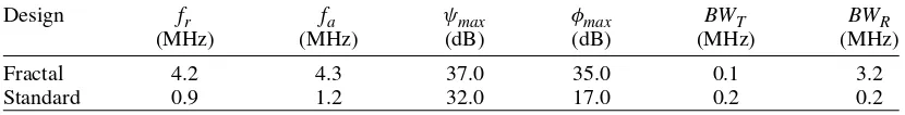
4. Results

As a result of the equations presented above, a comparison between the key operating characteristics of the transmission and reception spectra of the fractal and standard (Euclidean) designs (Hayward, 1984) can now be evaluated and compared. The key parameters of interest to be compared between both models include the amplitude (or gain) and the bandwidth (the range of frequencies over which a certain gain, expressed in decibels, is exceeded). To evaluate the transmission and reception sensitivities of the fractal device, the fractal generation levels were gradually increased and the differences in these parameters observed. However, with the aim of physically producing the device, we will focus on the fractal generation level n = 3. From a practical perspective, these fractal transducers will only be able to be manufactured at low fractal generation levels. To perform a fair comparison, the volume of piezoelectric material in the standard design (vol_E)and fractal design(vol_F)is kept consistent. The volume of the piezoelectric material in the standard design is vol_E=L2d_E=LA_E, where L is the length of the front face, d_Eis the thickness and A_Eis the area occupied by the electrode. The volume of the piezoelectric material in the fractal design is vol_F =S_nd_F, where S_nis the area of the front face of the fractal piezoelectric design at generation level n (the black area in Fig.6) and d_F is the thickness; the area Snis then given by Sn=

√

3L21−(3/4)n+1/4 and equating volEand volFgives dF=L2dE/Sn.

The fractal transducer has one electrode of area A_F =dFh(n)/2 at one face and two electrodes of area

A_Feach on the opposite face (see Fig.6). As the device operates essentially as a capacitor in this circuit, and since the total capacitance of two capacitors in parallel is just the sum of those two capacitances, then we take the total area to be A_F = 2A_F = d_Fh(n) _{= d}

FL/2n. By choosing a particular value for

the fractal generation level n, the thickness d_E and the length L, this sets d_F, which in turn sets A_E, A_F and the volume of piezoelectric material. The behaviour of the device is dictated by its electrical

Fig. 6. A three-dimensional schematic of the Sierpinski gasket ultrasonic transducer at fractal generation level n=2. The black triangles are the front faces of the piezoelectric material. The device is connected to an electrical circuit as shown where each electrode has surface area A_F.

Fig. 7. Non-dimensionalized electrical impedance (equation (3.14)) versus frequency for the SG transducer at fractal generation level n=3 (dashed line). The non-dimensionalized electrical impedance of the standard (Euclidean) transducer (Hayward, 1984) is plotted for comparison (full line). Parameter values are given in Table1.

resonances, which in turn depend on its capacitance. The capacitance depends on the distance between the electrodes, which remains fixed in the conventional design. So, to assist in the comparison between the standard design and the fractal design, the distance between the electrodes was held fixed in the fractal case too. A different scenario could be studied where the surface area remains fixed and the edge length L is varied. To enable a frequency domain analysis, we set q→σ +jωwhereσ,ω∈R,σis a damping term (set to zero in this paper),ωis the angular frequency and j is the square root of−1. The characteristic profile of the electrical impedance spectrum (magnitude) for both models where n = 3 is illustrated in Fig.7. The fractal design, given by (3.14), is represented by the dashed line while the equivalent standard design is represented by the full line (Hayward, 1984). It can be seen that the behaviour is predominantly that of a capacitor it decreases according to a 1/(C0f)profile where C0 is the capacitance and f is the frequency with a few resonant peaks superimposed on this. From the above analysis, A_E=√3(1−(3/4)n+1)2(n−3)_A

Fand the coefficient of AFis monotonically

increasing as a function of the fractal generation level n and is greater than one for all n3. Hence,

Table 1 Parameter values for the front and back mechanical loads and the electrical load (Mulholland et al., 2007;Mulholland & Walker, 2011)

Design parameter Symbol Magnitude Dimensions

Parallel electrical impedance load Z_P 1000 Ohms

Series electrical impedance load Z0 50 Ohms

Length of SG L 1 mm

Mechanical impedance of the front load Z_L 1.5 MRayls

Mechanical impedance of the backing layer ZB 2 MRayls

Wave speed in the front load cL 1500 ms−1

Wave speed in the backing layer cB 1666 ms−1

Density of the front load ρ_L 1000 kgm−3

Shear modulus of the front load μ_L 2.25×109 Nm−2

Shear modulus of the backing layer Y_B 2.78×109 Nm−2

Thickness of the piezoelectric material

in the standard (Euclidean) design dE 10 mm

Fig. 8. Non-dimensionalized transmission sensitivity (equation (3.15)) versus frequency for the SG transducer at fractal generation level n= 3 (dashed line). The non-dimensionalized transmission sensitivity of the standard (Euclidean) transducer (Hayward, 1984) is plotted for comparison (full line). Parameter values are given in Table1.

for reasonable values of n, AE AF. Since C0 = AE/Fε11/L, then C0E C0F (where C0E/F is the

capacitance in the E-standard / F-fractal design) and so 1/(C_0Ef) 1/(C_0Ff). Since the standard design has a larger capacitance, then this explains why its electrical impedance is in general lower. The locations and magnitudes of the first maximum ( fa) and first minimum ( fr) turning points are the critical

features for a design engineer. In transmission mode, the device should be driven at the mechanical resonance frequency (the frequency at the first minimum) where it will deliver the maximum force on the load. In reception mode however, the device should be driven at the frequency of the first maximum (the electrical resonance frequency). As shown in Fig.7, for the standard design (full line) fr = 0.9

MHz,| ˆZ_E(f_r)| = 34 dB, f_a =1.2 MHz and| ˆZ_E(f_a)| =51 dB. As discussed above, these frequencies correspond precisely to the first maximum in the transmission sensitivity plot (Fig.8; full line) and the reception sensitivity plot (Fig.9; full line).