Multiple-time-scale analysis for pinned breathers in Bose-Hubbard chains

in Bose-Hubbard Chains

SUPA and Department of Physics, University of Strathclyde, Glasgow G4 0NG, Scotland, EU

(Dated: January 29, 2019)

Localized and pinned discrete breathers in Bose-Einstein Condensates in optical lattices or in arrays of optical waveguides, oscillate with frequencies which are much higher than those present in the spectrum of the background. Hence, the interaction between localized breathers and their surroundings is extremely weak leading to a multiple-time scale perturbation expansion. We identify the leading order in the asymptotic expansion of the breather amplitude which does not average to zero after one full oscillation. The reduced model predicts a lower bound of the breather drift-times and explains the topological differences between breathers in dimers, trimers and in spatially extended one-dimensional lattices even in the presence of transport from boundary heat-baths. These analytical boundaries hold true for lattices of any length, due to the highly localised nature of breathers.

PACS numbers: 63.20.Pw, 03.75.Lm, 05.60.-k

I. INTRODUCTION

Bose-Einstein condensates (BEC) trapped in an opti-cal lattice have attracted an enormous scientific inter-est since they provide excellent control of the quantum and supefluid phases of ultra-cold atoms [? ? ]. These benefits have led to important realizations of analogues of solid-state phenomena such as quantum phase transi-tions [? ], transport [? ], Anderson localization [? ] and macroscopic Zeno effect [? ]. In the superfluid phase of the BEC, a lot of attention has been devoted to the case of deep optical lattices where expansions of the wave-function in Wannier wave-functions and discrete models of the lattice structure have wide and well tested validity. In one dimensional lattice configurations, the dynamics of the BEC cloud is well described by the discrete nonlinear Schr¨odinger equation (DNLSE) [? ] that can be directly derived from a Bose-Hubbard lattice Hamiltonian. One fascinating aspect is that the DNLSE has been originally used to describe light propagating in arrays of optical waveguides and even protein systems in biophysics [? ? ]. Important and universal nonlinear features of the conser-vative DNLSE are modulational instabilities and discrete breathers [? ]. Discrete breathers are spatially localized modes that own their stability to the discreteness of the lattice and that oscillate in time with a well determined frequency [? ? ? ].

When simulating BEC in optical lattices with the DNLSE, discrete breathers are favoured in the presence of repulsive atomic interactions that are typical, for ex-ample, of 87_{Rb atoms. Several methods have been} sug-gested for the generation of discrete breathers in the DNLSE including the evolution from Gaussian wavepack-ets [? ? ] and the relaxation from random phase states via localized losses [? ].

Breathers have been mostly investigated in the pres-ence of small backgrounds, when perturbative techniques

can be developed to determine their stability [? ? ]. Here we focus on the properties of localised solutions in the presence of a large (orderO(1)) fluctuating background. The background can either evolve in an isolated setup, where the total energy and mass are conserved, or after including the interaction with suitable thermostats. In the latter case, the action of the heat baths is mimicked by implementing stochastic Langevin equations like in [? ], where the temperature and the chemical potential of the background are given by the parameters of the reser-voir.

Without loss of generality, we introduce a singular per-turbation expansion for tall breathers in contact with a large background on one of their sides only. This simpli-fied set up allows for the direct integration of analytical yet implicit expressions. As demonstrated by the com-putational tests, the analytical findings can be extended to breathers in contact with a background on both sides, to lattices of any length, and under a large variety of configurations, i.e. periodic boundary conditions (PBC), reflecting boundary conditions (by imposing zeros at the ends of the Bose-Hubbard chain) or in contact with heat baths at the chain’s ends.

In an ideal breather, the tails are perfectly synchro-nised with the oscillations at its peak and decay expo-nentially fast along the lattice. When the background is large, however, this synchronisation is destroyed and the dynamics of the background follow trajectories which are much slower than the breather oscillation. For large enough backgrounds, the breather’s tails are completely covered by and indistinguishable from the background: in practice the localized solution occupies just a single site in the lattice. Even under these conditions, it is pos-sible to investigate the stability of the localized solution and to determine the perturbations induced by the back-ground on the breather.

surroundings by determining the leading perturbative or-der at which there is a change in the breather size af-ter one oscillation period. Our work sheds light on the mechanism of adiabatic decoupling between localized so-lutions and their surroundings, leading to a analytical expressions that quantify the slow drifts in the breather amplitude due to the very weak interactions between the breather and its neighbours. In sections II, III, and IV we present the multiple-scale analysis based on the perturba-tion expansion in the inverse of the breather frequency. By averaging over one period of the breather rotation, we obtain in V the core equation that describes the ex-tremely slow dynamics of the breather amplitude. The theory is successfully compared with numerical simula-tions in section VI where we show its independence of the lattice length and application to infinitely-extended backgrounds. We also show that trimer and dimer config-urations are topologically different from more extended systems, and that they display a higher degree of stabil-ity. Conclusions and future developments are presented in section VII.

II. PERTURBATION EXPANSION

The DNLSE is a useful model to study quantum trans-port phenomena in BEC but also light diffraction in ar-rays of optical waveguides or biochemical systems such as biopolymers [? ] and proteins [? ]. Here we consider a BEC in a deep optical lattice with repulsive interactions. The evolution of the complex wave-functionzj =xj+iyj

at site j follows from the Bose-Hubbard Hamiltonian [? ]

HBH = N−1

X

j=0

|zj|4+z∗jzj+1+zjzj∗+1), (1)

where N is the number of sites and 0 ≤ j < N. The evolution equations are

dzj

dt ≡dtzj= 2i|zj| 2_z

j+izj−1+izj+1; (2)

where the timetis dimensionless [? ],z−1= 0, while the boundary conditions inj=N will be discussed later on. In this paper we investigate a set up where a tall breather sits inj= 0, i.e. we set |z0(0)|2_{=I1, to be} compared with a background of amplitude orderO(1). It is well known that the breather will eventually decay on a time scale that depends on its heightfor positive tem-peratures. Our numerical simulations confirm this fact and show that the life time of a breather increases expo-nentially with its initial mass (|z0(0)|2 =I) when

keep-ing the average background fluctuations fixed. There-fore, given enough time, all breathers will encounter a non-perturbative excitation that will destabilise them. The work done here focuses on the laminar part of the breather evolution, where the mass of the breather barely

changes. In the case of rare turbulent events, the breather changes size suddenly and the perturbative approach can-not be employed any longer. We tackle thelaminar prob-lem with a perturbative approach where the smallness parameter is not the background amplitude, as previ-ously considered [? ], but the inverse of the breather amplitude.

Upon expressing the breather state into polar coor-dinates, z0 ≡ A0eiψ0, while using a standard Cartesian representation for the other lattice sites (zj =xj+iyj,

j≥1) the breather evolution can be written as

dtA0=x1sinψ0−y1cosψ0 (3) dtψ0= 2A20+A

−1

0 (x1cosψ0+y1sinψ0). (4) From this representation it is transparent that ifA01, the phaseψ0rotates very rapidly with a frequency given byω≈2A2

01. From now on,ε= 1/ωis considered to be a smallness parameter for the development of a suit-able perturbative approach. By introducing the “slow” phaseφ0=ψ0−ωt, the DNLSE can be written as

dtA0 = x1sin(ωt+φ0)−y1cos(ωt+φ0) dtφ0 = 2A20−ε−1+A0−

1

x1cos(ωt+φ0)+ +y1sin(ωt+φ0)

dtx1 = −2(x21+y12)y1−y2−A0sin(ωt+φ0) dty1 = 2(x21+y21)x1+x2+A0cos(ωt+φ0) dtxj = −2(x2j+y

2

j)yj−yj−1−yj+1 j≥2 dtyj = 2(x2j+y

2

j)xj+xj−1+xj+1 j≥2. (5)

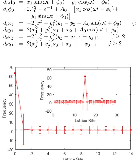
FIG. 1. Average oscillation frequency of a large breather in j= 0 and its background from simulations of Eq. (2) with a heat-bath at infinite temperature in j = 15. The error bars quantify the fluctuations of the oscillation frequency over 3×104 _{time units. The dashed black line shows that the}

average frequencies of the background are close to a common value given by 2×h|zB|2i, whereh|zB|2iis the mean amplitude

generated by the Langevin heat-baths. The inset, shows the average oscillation frequency of a breather with background at both sides.

coordinates and the background sites in Cartesian coor-dinates. Fig. 1 shows the average oscillation frequency in a lattice of 15 sites with a breather of amplitude|z|= 6 in j= 0 and in a lattice of 31 sites with a breather of ampli-tude|z|= 6 in the middle (see inset). The lattice bound-aries are in contact with Langevin heat-baths at infinite temperature [? ]. One can see that the background ther-malises to a common frequency with roughly the same size of fluctuations, therefore justifying the choice of the hybrid polar-Cartesian basis. Remarkably enough, the frequency of the breather is very stable around the value 2|z|2 _{≈ 72. This in turn, justifies the choice of the} def-inition of the smallness parameter. The only sites that have frequency statistics different from the background are the nearest neighbours of the breather, which, as it will emerge later in this work, contain rapidly oscillating components at low orders in their asymptotic expansions. The perturbative approach is developed for breathers in contact with backgrounds only on one side and is then extended to the generic case when the breather sits at a random lattice site and is perturbed by small excitations arriving from backgrounds on both sides. Fig. 1 shows that there is a clear separation of time scales due to the much faster oscillation of the breather with respect to its surrounding.

Two time scales appear naturally in the system: a short one of order ε = 1/ω associated to the fast ro-tation of the breather’s phase and a “long” one of order

O(1) associated to the fluctuating motion of the back-ground. The most appropriate way to handle this kind of problems is to consider multiple time scales by intro-ducing two time variables and thereby by rewriting the time derivative as

dt=ε−1∂t1+∂t2, (6)

where t1 and t2 represent the fast and slow time scales, respectively [? ].

Before proceeding with the formal expansion, it is use-ful to go back to Eq. (5) to estimate the variation of the different variables over a time scale of order ε. It is legitimate to assume that the time dependence of the fields is due to the fast rotation ω and thereby neglect the variation of all the variables appearing in the r.h.s. of the above equations. Upon integrating Eq. (5) for a

time ∆t=εone obtains

∆A0 ≈ −εx1cos(ωt+φ0) +y1sin(ωt+φ0)

≈ O(ε) ∆φ0 ≈ εA−01

x1sin(ωt+φ0)−y1cos(ωt+φ0)

≈ O(ε3/2)

∆x1 ≈ −ε2(x12+y21)y1+y2

+ +εA0cos(ωt+φ0)

≈ O(ε1/2₎ ∆y1 ≈ ε

2(x2

1+y12)x1+x2

+ +εA0sin(ωt+φ0)

≈ O(ε1/2₎ ∆xj ≈ ε

−2(x2_j+y_j2)yj−yj−1−yj+1

≈ O(ε) ∆yj ≈ ε

2(x2_j+y_j2)xj+xj−1+xj+1

≈ O(ε)

(7)

These results suggest that any asymptotic expansion with respect to ε should include half-integer powers (i.e. it should be done with respect to√ε) and also provide in-formation on where the series should start for each vari-able. More precisely, we consider a perturbation expan-sion given by

A0 ∼ ε− 1/2_A[−1]

0 +

P

m≥2ε

m/2_A[m] 0 t1, t2

φ0 ∼ φ [0] 0 +

P

m≥3ε

m/2_φ[m] 0 t1, t2

x1 ∼ x [0] 1 +

P

m≥1ε

m/2_x[m] 1 t1, t2

y1 ∼ y [0] 1 +

P

m≥1ε

m/2_y[m] 1 t1, t2

xj≥2 ∼ x [0]

j +

P

m≥2ε

m/2_x[m]

j t1, t2

yj≥2 ∼ y [0]

j +

P

m≥2ε

m/2_y[m]

j t1, t2

.

(8)

This perturbation is singular, since it includes the di-verging termε−1/2_A[−1]

0 (t2). This follows from our initial assumption of dealing with tall breathers.

By inserting the power expansion (8) into Eq. (5) and by a further Taylor expansion of the sinusoidal functions, we are able to split each equation into a series of separate conditions for the different powers of√ε. Our target is to quantify the weak coupling between the breather and its surroundings, by looking for the first term in the expan-sion of the breather amplitude which does not average to zero over one full rotation. Finding an analytical ex-pression for this term would not only quantify the order of magnitude of the slow derivative, but it would also provide an upper bound of diffusive processes and char-acterise the size and nature of the breather ’tails’ in the presence of large backgrounds. The pinned breather is extremely localised and only the nearest neighbour con-tributes directly to the slow drifts of the breather mass. At lowest order√ε, we find:

∂t1A [−1]

0 = 0

∂t2A [−1]

0 = 0

∂t1φ [0]

0 = −1 + 2(A [−1] 0 )

2

∂t2φ [0]

0 = 0

∂t1x [0]

j = 0 j ≥1

∂t1y [0]

j = 0 j ≥1.

The first two equations show thatA[₀−1] is a constant. With our initial choice A[₀−1] = 1/√2, it turns out that φ[0]₀ is a constant as well. The last couple of equations tell us that the leading contributions of the background variables are slow for all sites withj6= 0.

For the breather wave-function, one obtains the follow-ing differential equations for the amplitude and the phase of the oscillatory motion.

At order 1 we find:

∂t1A [2]

0 = x

[0]

1 sin(t1+φ [0] 0 )−

−y₁[0]cos(t1+φ[0]₀ ). (10)

At orderε1/2 _{we find:}

∂t1A [3]

0 = x

[1]

1 sin(t1+φ [0] 0 )−

−y[1]₁ cos(t1+φ[0]₀ ) ∂t1φ

[3]

0 = 4A [2] 0 A

[−1]

0 +

x[0]₁ cos(t1+φ[0]₀ )+ +y[0]₁ sin(t1+φ[0]₀ )

/A[₀−1].

(11)

At orderεwe find:

∂t2A [2] 0 +∂t1A

[4]

0 = x

[2]

1 sin(t1+φ [0] 0 )−

−y₁[2]cos(t1+φ [0] 0 ) ∂t1φ

[4]

0 =

x[1]₁ cos(t1+φ[0]₀ )+ +y₁[1]sin(t1+φ₀[0])/A[₀−1] .

(12)

At orderε3/2 _{we find:}

∂t2A [3] 0 +∂t1A

[5]

0 = φ

[3] 0 x

[0]

1 cos(t1+φ [0] 0 )−

−y[3]₁ cos(t1+φ[0]₀ )+ +x[3]₁ sin(t1+φ[0]₀ )+ +φ[3]₀ y₁[0]sin(t1+φ

[0] 0 ).

(13)

Finally, at orderε2 _{we find:}

∂t2A [4] 0 +∂t1A

[6]

0 = φ

[4] 0 x

[0]

1 cos(t1+φ [0] 0 )+ +φ[3]₀ x[1]₁ cos(t1+φ

[0] 0 )−

−y[4]₁ cos(t1+φ[0]₀ )+ +x[4]₁ sin(t1+φ[0]₀ )+ +φ[4]₀ y₁[0]sin(t1+φ

[0] 0 )+ +φ[3]₀ y₁[1]sin(t1+φ

[0] 0 ).

(14)

We will see that the first order at which the breather derivative does not average to zero isO(ε2). In order to prove this fact, one must solve the coupled differential equations for all orders lower than ε and determine the corresponding expressions of the expansion terms.

The same procedure gives rise to the differential equa-tion for the real and imaginary parts of the wave-funcequa-tion at sitej= 1, the site close to the breather.

At orderε−1/2 _{we find:}

∂t1x [1]

1 = −A [−1]

0 sin(t1+φ [0] 0 ) ∂t1y

[1]

1 = +A [−1]

0 cos(t1+φ [0] 0 ).

(15)

At order 1 we find:

∂t2x [0] 1 +∂t1x

[2]

1 = −2y [0] 1 (x

[0] 1

2

+y₁[0]2)−y₂[0] ∂t2y

[0] 1 +∂t1y

[2]

1 = +2x [0] 1 (x

[0] 1

2

+y₁[0]2) +x[0]₂ . (16)

The last two equations contain the DNLSE on the RHS. From the initial assumption, these equations suggest that ∂t1x

[2]

1 = 0, which means that bothx [2] 1 andy

[2]

1 are slow. One can iterate the procedure and obtain increasingly more complex formulas for the higher order terms of the expansions ofx1 andy1.

For generic sites, (16) at order 1 reduces to:

∂t2x [0]

j +∂t1x [2]

j = −2y

[0]

j (x

[0]

j

2

+y[0]_j 2)− −y_j[0]₋₁−y_j[0]₊₁

∂t2y [0]

j +∂t1y [2]

j = +2x

[0]

j (x

[0]

j

2

+y[0]_j 2)+ +x[0]_j−1+x[0]_j+1

(17)

which leads to the same conclusion thatx[2]_j andy_j[2]are slow variables which will be used extensively while per-forming averaging later in the work.

III. FIRST NON-TRIVIAL TERMS

The differential equations at specified orders of the per-turbations need to be integrated to obtain the dynamical expressions of the perturbative terms. In doing this, slow terms appear as integration constants. The solvability condition is then imposed by the requirements that the energy and the norm have to remain conserved at any given order of the perturbation.

We have seen above how to obtain non-trivial differen-tial equations for the breather and its nearest neighbour. By integrating Eqs. (10)-(15) and making use of the fact that the background is slow andA[₀−1] and φ[0]₀ are con-stants, we obtain,

A[2]₀ = −x[0]₁ cos(t1+φ [0] 0 )−y

[0]

1 sin(t1+φ [0] 0 )+ +C1(t2)

x[1]₁ = A[₀−1]cos(t1+φ [0]

0 ) +C2(t2) y[1]₁ = A[₀−1]sin(t1+φ

[0]

0 ) +C3(t2)

(18)

whereC1(t2),C2(t2) andC3(t2) are slow functions to be determined.

Meanwhile, we know that the Hamiltonian of the sys-tem is, at orderO(ε−1/2_),

H_O(1/√

ε) =

√

2

A[2]₀ +x[0]₁ cos(t1+φ [0] 0 )+

+y[0]₁ sin(t1+φ[0]₀ ) (19)

where we have made use of the equalityA[₀−1] = 1/√2. Upon substituting the analytical expression forA[2]₀ in (18) one obtains:

HO(1/√ε)=

√

which requires C1 to be constant to guarantee that the Hamiltonian is conserved. This constant is zero, since any other value would induce secular terms when inte-grating higher order terms.

By imposing the conservation of norm at order√εwe obtain the additional constraint:

x[0]₁ C2(t2) +y [0]

1 C3(t2) = 0. (21) Therefore the two unknown slow functions must satisfy

C2(t2) = −Ky [0] 1

C3(t2) = Kx[0]₁ , (22) whereK is a real number to be determined.

The differential equation forx1 at orderO(ε1/2_{) reads}

∂t1x [3] 1 +∂t2x

[1]

1 =−2(x [0] 1 x

[1] 1 y

[0] 1 + +x[0]₁ 2y[1]₁ + 3y[0]₁ 2y[1]₁ ).

(23)

Replacingx[1]₁ andy₁[1]with their analytical expressions from (18) one arrives at

∂t1x [3]

1 +∂t2C2= =−2[x[0]₁ y₁[0](A[₀−1]cos(t1+φ

[0]

0 ) +C2)+ +(x[0]₁ 2+ 3y₁[0]2)(A[₀−1]sin(t1+φ

[0]

0 ) +C3)].

(24)

From this it follows that the most general form that x[3]₁ can have is D1(t2) +D2(t2)×t1+D3(t2) sin(t1+ φ[0]₀ ) +D4(t2) cos(t1+φ[0]₀ ). The Hamiltonian at order

O(ε) contains terms of the sort A[₀−1]x[3]₁ cos(t1+φ[0]₀ ) and A[₀−1]y₁[3]sin(t1+φ[0]₀ ) in addition to a plethora of terms which can all be written asB1(t2) +B2(t2) sin(t1+ φ[0]₀ ) +B3(t2) cos(t1+φ[0]₀ ) +high harmonics. This im-plies that the Ansatze of x[3]₁ and y₁[3] are of the type B1(t2) +B2(t2) sin(t1+φ

[0]

0 ) +B3(t2) cos(t1+φ [0]

0 ), which means thatD2(t2) = 0. Isolating only the slow terms of equation (2) one arrives at

∂t2C2(t2) =−2

h

2x[0]₁ y[0]₁ C2(t2)+

+C3(t2) x [0] 1

2

+ 3y[0]₁ 2i

.

(25)

Using the constraint (22) and making all possible sim-plifications leads to:

Kx[0]₂ = 0 (26) which implies that K must be zero for extended lat-tices where x[0]₂ 6= 0. The slow terms that appear from the integration over the fast time scale are all zero, i.e. C1(t2) =C2(t2) =C3(t2) = 0 so that, Eq. (18) reduces to

A[2]₀ = −x[0]₁ cos(t1+φ [0] 0 )−y

[0]

1 sin(t1+φ [0] 0 ) x[1]₁ = A[₀−1]cos(t1+φ[0]₀ )

y₁[1] = A₀[−1]sin(t1+φ[0]₀ ).

(27)

By using these solutions, it becomes apparent that the second equation in (12) simplifies to∂t1φ

[4]

0 = 1. This fast term appears because in the differential equation of the slow phase there is the term 2A2

0−ωwhich has a first non-zero component at orderε.

The expressions (27) can now be averaged over one full rotation by making use of the fact thatx[0]₁ andy[0]₁ are slow and thatA[₀−1] is time-independent,

R2π

0 dt1A [2] 0 = 0

R2π

0 dt1x [1]

1 = 0

R2π

0 dt1y [1]

1 = 0

(28)

Therefore, the first non-trivial terms are zero when aver-aged over one full rotation for both the breather and its nearest neighbour. In order to quantify the coupling be-tween breather and background, one is therefore forced to continue the perturbative analysis to higher orders as shown below.

IV. HIGHER ORDER TERMS

Having seen how to proceed with the perturbation ex-pansion, i.e. by writing of the differential equations at different orders of the expansion for the breather, its neighbour and the background lattice, by integrating these differential equations and by using the expressions of the lower order terms, we provide here the final re-sults corresponding to the application of this procedure to terms in the expansion of order higher than those seen in Section III. These are:

A[3]₀ = 0

A[4]₀ = −M(t2) cos(t1+φ [0] 0 )−

−N(t2) sin(t1+φ[0]₀ ) A[5]₀ = P(t2)−y₁[0]cos(φ[0]₀ +t1)+

+x[0]₁ sin(φ[0]₀ +t1)+ + 3

2√2

x[0]₁ 2−y₁[0]2cos[2(φ[0]₀ +t1)]+ 3√2x[0]₁ y[0]₁ cos(φ[0]₀ +t1) sin(φ[0]₀ +t1) x[2]₁ = −∂t2y

[0]

1 +M(t2) x[3]₁ = +2 x[0]₁ 2+ 3y[0]₁ 2

A[₀−1]cos(t1+φ [0] 0 )

−4x[0]₁ y[0]₁ A₀[−1]sin(t1+φ [0] 0 ) y₁[2] = ∂t2x

[0]

1 +N(t2)

y₁[3] = +2 3x[0]₁ 2+y[0]₁ 2A[₀−1]sin(t1+φ[0]₀ )

−4x[0]₁ y[0]₁ A₀[−1]cos(t1+φ[0]₀ ) φ[3]₀ = 4A[₀−1]− 1

A[₀−1]

[−x[0]₁ sin(t1+φ[0]₀ ) +y₁[0]cos(t1+φ[0]₀ )] +P(t2)

φ[4]₀ = t1+Q(t2)

(29)

whereM(t2),N(t2),P(t2) and Q(t2) are slow functions to be determined.

A. Solvability Conditions

We are now able to use analytical expressions of per-turbation terms above in the evaluation of the norm and the energy (Hamiltonian) of the system. We start by considering the dimer (abbreviated by the superscriptD) formed by the breather and its first neighbourj= 1:

ND _{= ε}−1_A[−1] 0

2

+A[0]₁ 2+

+εA[₀−1]2+ 2(x[0]₁ x[2]₁ +y₁[0]y[2]₁ )+ +O(ε3/2₎

HD _{= ε}−2_A[−1] 0

4

+A[0]₁ 4+εh−8A[0]₁ 6+

+A[0]₁ 2 15 2 −4(x

[0] 1 x

[0] 2 +y

[0] 1 y

[0] 2 )+ 4(x[0]₁ M+y[0]₁ N)i

+O(ε3/2₎

(30)

Here, it is more convenient to express the zero-order wave-function using polar coordinates via the transfor-mation: x[0]_j →A[0]_j cos(ψ_j[0]) andy[0]_j →A[0]_j sin(ψ[0]_j ).

Similar calculations can be done for the rest of the Bose-Hubbard lattice, and then one must impose the constraint that the fluxes of norm and energy from the background cancel those coming from the dimer at all orders. An important consideration is that when one de-fines the Hamiltonian of the background, the coupling between sitesj= 1 andj= 2 must also be included. For the terms at orderε in the background (abbreviated by the superscriptB), one obtains:

NB

O(ε) = 2

P

j>1 x [0]

j x

[2]

j +y

[0] j y [2] j HB

O(ε) = 4

P

j>1

h

x[0]_j 2+y_j[0]2×

x[0]_j x[2]_j +y_j[0]y[2]_j i

+ +2P

j≥1 x [2]

j x

[0]

j+1+x [0]

j x

[2]

j+1+ +y_j[2]y_j[0]₊₁+y_j[0]y[2]_j+1

(31)

We now use the fact that background sites evolve slowly compared to the breather rotation (i.e. also the first correction is a slow function) and obtain

∂t2x [2]

j = −y

[2]

j−1−y [2]

j+1−2y [2]

j (3y

[0]

j

2

+x[0]_j 2)− −4x[2]_j x[0]_j y[0]_j

∂t2y [2]

j = +x

[2]

j−1+x [2]

j+1+ 2x [2]

j (3x

[0]

j

2

+y_j[0]2)+ +4y[2]_j x[0]_j y[0]_j

(32)

We determinex[2]₂ and y[2]₂ by imposing:

∂t2N

B

O(ε) = −∂t2N

D O(ε) ∂t2H

B

O(ε) = −∂t2H

D O(ε)

(33)

Note that ∂t2N

B

O(ε) and ∂t2H

B

O(ε) contain non-vanishing terms that come only from the contact with the breather and its nearest neighbours and not from the background.

By using the Cramer rule, we find that the two equa-tions are always linearly independent and that the dis-criminant of this system is strictly positive. After the algebraic operations are completed,

x[2]₂ = −17A

[0] 1 2 + 8A

[0] 1

5

cos(ψ[0]₁ )+

+4A[0]₁ 2A[0]₂ cos(2ψ[0]₁ −ψ[0]₂ )− −2A[0]₂ 3cos(ψ[0]₂ )−A[0]₃ cos(ψ₃[0])+ +∂t2N−4A

[0] 1

2 M−

2A[0]₁ 2[Mcos(2φ[0]₀ ) +Nsin(2φ[0]₀ )]

(34)

y₂[2] = −17A

[0] 1 2 + 8A

[0] 1

5

sin(ψ₁[0])+

+4A[0]₁ 2A[0]₂ sin(2ψ₁[0]−ψ₂[0])− −2A[0]₂ 3sin(ψ[0]₂ )−A[0]₃ sin(ψ₃[0])− −∂t2M−4A

[0] 1

2 N+

2A[0]₁ 2[Ncos(2φ[0]₀ )−Msin(2φ[0]₀ )]

The solvability conditions have been used to determine the expressions (34) forx[2]₂ andy[2]₂ . However, the func-tions M(t2), N(t2), P(t2) and Q(t2) cannot be deter-mined from the solvability conditions. These terms can-cel at all orders leading to the trivial relation 0 = 0. We show in the next subsection, however, that the explicit form of these functions is not necessary when determining the first differential equation in the perturbation expan-sion that does not average to zero over one period of the breather rotation.

V. AVERAGING OVER ONE PERIOD OF THE BREATHER ROTATION

Let us now introduce the notation

DA_ε2 ≡∂t2A [4] 0 +∂t1A

[6]

0 (35)

This is the lowest-order term providing an average non-zero slow contribution to the evolution of the breather mass. With the help of Eq. (14), replacing all the known functions with their explicit expressions, and af-ter averaging over one fast rotation (i.e. taking h∗i ≡

1 2π

R2π

0 (∗)dt1) we arrive at,

hDA_ε2i=x [0] 1 sin(φ

[0] 0 )−y

[0] 1 cos(φ

[0]

0 ) +P(t2)−

−hy₁[4]cos(t1+φ[0]₀ )i+hx[4]₁ sin(t1+φ[0]₀ )i

(36)

whereP(t2) is one of the unknown slow functions in the expression ofφ[3]₀ in Eq. (29) andx[4]₁ , y₁[4] are unknown high order terms for the wave-function of the nearest neighbour.

It is now useful to express hy₁[4]cos(t1 + φ[0]₀ )i and

From the expansion of the DNLSE at site j = 1, we write the differential equation for the derivative ofx1at orderε:

∂t1x [4] 1 +∂t2x

[2]

1 = −2x [1] 1

2

y[0]₁ −4x[0]₁ x[2]₁ y[0]₁ − −4x[0]₁ x[1]₁ y₁[1]−6y₁[0]y₁[1]2− −2x[0]₁ 2y[2]₁ −6y[0]₁ 2y[2]₁ − −A[₀−1]φ₀[3]cos(t1+φ[0]₀ )− −A[2]₀ sin(t1+φ

[0] 0 )−y

[2] 2

(37)

At this stage, one can replace all the known terms on the right hand side with their expressions from (29) and make all possible simplifications. In addition,∂t2x

[2] 1 can be substituted with its analytical expression and moved to the right hand side.

We integrate both sides with respect to the fast timet1. This leads to an analytical expression forx[4]₁ which con-tains the termsx[2]₂ , y₂[2], M(t2),N(t2) andP(t2) which are all slow functions. After integrating this equation, one finds thatx[4]₁ contains terms which are different from the other high order functions of (29) because they con-tain expressions of the typeF(t2)×t1. These terms ap-pear in the Hamiltonian at orderε3/2_{, together with the} known functionφ[4]₀ =t1+Q(t2) and the term A

[6] 0 .

The next required step is to calculatehx[4]₁ sin(t1+φ [0] 0 )i which again contains the slow terms x[2]₂ , y₂[2], M(t2), N(t2) andP(t2).

hx[4]₁ sin(t1+φ [0] 0 )i=−

A[₀−1]P

2 +

+

(

6A[₀−1]2y₁[0]+ 2

−4y[0]₁ (x[0]₁ 4+

+x[0]₁ x[0]₂ + 2x[0]₁ 2y₁[0]2+y[0]₁ 4)+

+(2x[0]₁ 2+x[0]₂ 2−2y₁[0]2)y₂[0]+

+y₂[0]3

+y[2]₂ +y₃[0]

)

cos(φ[0]₀ )

(38)

Analogously, one can obtain an expression for

hy₁[4]cos(t1+φ[0]₀ )i, and then express the average from

(36) as:

hD_εA2i = y [2] 2 cos(φ

[0] 0 )−x

[2] 2 sin(φ

[0] 0 )−

−2A[0]₂ 3sin(φ[0]₀ −ψ₂[0])+ +A[0]₁ h −2 + 8A[0]₁ 4

sin(φ[0]₀ −ψ[0]₁ )+ +4A[0]₁ A[0]₂ sin(φ[0]₀ −2ψ[0]₁ +ψ[0]₂ )i

−A[0]₃ sin(φ[0]₀ −ψ₃[0]) +∂t2M(t2) cos(φ

[0] 0 )+ +∂t2N(t2) sin(φ

[0] 0 )

−2A[0]₁ 2N(t2) cos(φ[0]₀ −2ψ₁[0])+ +M(t2) sin(φ[0]₀ −2ψ[0]₁ ) +4A[0]₁ 2N(t2) cos(φ[0]₀ )− −M(t2) sin(φ

[0] 0 )

(39)

We can now replacex[2]₂ andy₂[2]with their analytical expressions obtained in the previous subsection (see Eq. (34)) obtaining,

hD_εA2i= 13

2 A [0] 1 sin(φ

[0] 0 −ψ

[0]

1 ) (40)

It is quite remarkable that M(t2),N(t2) andP(t2) do not appear in the final expression of Eq. (40). This jus-tifies a posteriori the truncation of the calculations made in the application of the solvability conditions above. We also note that:

hD_εA2i=h∂t2A [4] 0 +∂t1A

[6]

0 i=h∂t1A [6]

0 i (41) and finally obtain

h∂t1A [6] 0 i=

13 2 A

[0] 1 sin(φ

[0] 0 −ψ

[0]

1 ). (42)

Eq. (42) is the main result of our work and is compared with numerical simulations of the DNLS in the next sec-tion.

VI. BREATHER FLUCTUATIONS AND

COMPARISON WITH SIMULATIONS

A. Decoupling due to the separation of time scales

again this analogy is only valid in the absence of rare events caused by very large fluctuations. The differential equation for the background becomes:

i∂t2z [0]

j6=0=−2

z

[0]

j

2

z_j[0]−z_j[0]₋₁−z_j[0]₊₁ (43)

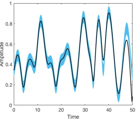
where z₀[0] ≡ 0 is a reflective boundary. Fig. 2 shows how the amplitude of the zero-order wave-function for the nearest neighbour of the breather obtained from Eq. (43) compares with that of the full solution of Eq. (2)). The slow function approximates the full trajectory very well for several hundred breather periods. After a while, the two trajectories separate due to the chaotic nature of the DNLSE. The reflective boundary approximation be-comes even more accurate when the size of the breather is increased, bounding the two trajectories close together for much longer times than those shown in Fig. 2. We note that these results are not conflicting with the work

of Flach et al. [? ] where a transmission coefficient for

a small amplitude plane wave interacting with a discrete breather is found to be of orderO(ε4_{) which is several} or-ders of magnitude higher than the relevant oror-ders of our perturbative analysis. Therefore, for our current analy-sis, the breather is simply a reflective boundary.

FIG. 2. Time evolution of the amplitude of the nearest neigh-bour on the right of the breather obtained by integrating the DNLSE Eq. (2) (light blue strip) and from the zero-order re-duced equation (43) (black line). Replacing the breather with a reflective boundary produces a similar dynamics of the back-ground. The breather had an initial amplitude of|z0|= 6 and

sat in the middle of a 15 sites lattice which was thermalised at infinite temperature and had the average occupation number h|zj|2i= 0.5. Analogous decouplings occur for both the left

and the right neighbours.

Backgrounds characterised by low temperatures tend to be less fluctuating and therefore, in their presence, this breather/vacancy analogy is satisfied over significantly

longer time scales. It is however worth noting that even for high-temperature backgrounds, one can still obtain results for the breather fluctuations and for the back-ground dynamics similar to those of Fig. 2 when using the simplified equation (43). As it will be seen later in this work, one can build a decoupling theory which is valid for times far longer than the separation time seen in Fig. 2, since it is possible to express the fluctuations in the breather size as a function of the zero-order back-ground at any given time, regardless of what the initial condition is. In order to build this theory however, it is crucial to use the adiabatic decoupling between the zero-order wave-function of the background and the breather oscillations.

This type of decoupling is also addressed in [? ] where it is shown that breathers induce weakly non-ergodic dy-namics. These localised solutions split the lattice into mutually disconnected regions, thermalised at different chemical potentials and different temperatures.

A clear evidence for the separation of the two time scales is also presented in Fig. 3. There, one can see that the background evolves over time scales of O(10), while the breather height is effectively frozen over scales of this magnitude. In addition, the sites in the back-ground frequently reach amplitudes which are close to zero, even if their overall size is of orderO(1). This pro-vides an additional justification for the choice of a hybrid polar-Cartesian system, which was introduced to avoid diverging derivatives for small values of the background amplitudes. From Fig. 3 one sees that the first neigh-bour (red line) displays a fast component of oscillation that comes from the breather. This component originates in the first non-trivial terms identified in Eq. (18). Note that the breather amplitude does not display any visible variations during times which characterise the evolution of the slow background.

B. Size of fluctuations

The amplitude of the breather fluctuates in time around a constant value ε−1/2_A[−1]

0 . For low orders of ε, the fluctuations average to zero over one fast rotation. More remarkably, our calculations are able to determine the magnitude of the slow perturbation which does not cancel over one fast oscillation. These slow drifts in the derivative of the breather norm appear at orderO(ε2_), and for lattices with more than three sites (N >3) are given by:

hdtA0i= 13

2 ε 2_A[0]

1 sin(φ [0] 0 −ψ

[0] 1 ) +O(ε

5/2_{) (44)}

FIG. 3. Time evolution of the amplitude of a breather in j= 0 (blue) and those of its two nearest neighbours (j= 1 in red, andj= 2 in black) for a lattice of 7 sites in contact with a heat-bath at positive temperature at one end from Eq. (2).

cancelling out after imposing the solvability conditions (33).

Note that Eq. (44) has been derived for breathers in contact with a background on one side only. Extensions to a more generic configurations require a sum of both left and right contributions

hdtA0i= 13

2 ε

2 X

j=±1

A[0]_j sin(φ[0]₀ −ψ_j[0]) +O(ε5/2_{). (45)}

This is an approximation since in the case of breathers in contact with backgrounds on both sides, there are two solvability conditions for four unknown high order functions and mixed terms of left and right backgrounds. These terms and the flow of energy from one side of the breather to the other are negligible so that the derivative of the breather norm only contains two contributions of the type shown in Eq. (44).

For lattices of length N > 3, we run computational simulations and record the evolution ofA0(t1, t2). This variable contains numerous high order terms which av-erage to zero over one full oscillation of the breather. In order to extract the slow drifts, one must take the Fourier Transform of A0, apply a Heaviside step func-tion filter, and then take the inverse Fourier Transform. Analogously, one applies the same algorithm onA1(t1, t2) to obtain a numerical approximation of the zeroth order amplitude of the nearest neighbour.

Let Πf(X) denote a low-pass filtered version of a signal

X, f being the cut-off frequency: all frequencies above this value are filtered out before applying, the inverse Fourier Transform. The averaged equation (44) implies

that:

−2π13 2 ε

3_Π

f(A1)≤Πf(A0)≤2π 13

2 ε 3_Π

f(A1) (46)

where one has used that−1 ≤ sin(x) ≤1 ∀x∈ R and also the properties of the Fourier transforms for deriva-tivesF(X0) =iωF(X). The analytical predictions given by the multiple time scale analysis can therefore be tested by checking the truthfulness of (46). A similar idea is pre-sented in [? ], where the authors make analytical predic-tions on the behaviour of a multiple scale system, which are ultimately confirmed by computational tests which consist of numerical filtering.

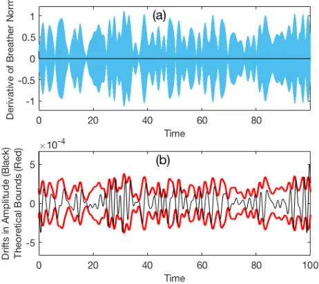
FIG. 4. Time evolution of dt|z0| over a time span of 100

time units. (a)dt|z0|from the numerical integration of Eq.

(2) (pale blue curve) and after the fast oscillating components have been filtered out (black line). (b) Same as (a) but magni-fied by a factor of 5000 (black line) with the analytical bounds from the inequalities (46) (red lines).

In order to test the accuracy of (42), (44) and (45), we focus on the fluctuations of the time derivative of the breather amplitude (dt|z0|), as shown in Fig. 4. This

test shows the evolution ofdt|z0|over a time span of 100

time units for a breather of initial size|z0|= 5,in contact with a background generated by a Langevin heat-bath at temperatureT = 3 and chemical potentialµ=−3.4. In our simulations, we have set a buffer zone of seven sites between the breather, situated at site j = 0, and the heat-bath located at site j = 8. In Fig. 4 (a), one can see that the fluctuations of the time derivative of the breather norm from the integration of Eq. (2) are of orderO(1). This is not surprising, since when applying the two-scale differential operatorε−1∂t1+∂t2on the first non-trivial term from (27) one obtains a contribution of the formε−1∂t1 εA

[2] 0

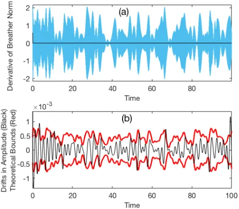
the norm, however, vanishes when averaged over one full rotation. In order to see only the slow components of the derivative, one must use numerical low pass filters. Fig. 4 (b) displays the same quantity, dt|z0|, but after the application of the numerical low pass filter and suit-able magnification. The same black curve is also shown in the upper diagram, where due to the large difference in the magnitude of the fluctuations, it appears to be al-most flat. What is remarkable is the excellent agreement between the slow fluctuations given by the numerical in-tegration of Eq. (2) and the analytical boundaries pre-dicted by the inequalities of Eq. (46). The extension of formula (44) to symmetric backgrounds is tested in Fig. 5. Similar tests have been ran for hundreds of configu-rations, by varying the initial height of the breather and the parameters of the heat-baths. For both positive and infinite temperature Langevin heat-baths, the evolution of the breather norm remains confined between bound-aries that are very well approximated by those defined in equation (45).

FIG. 5. Same as Fig. 4 but for a breather with backgrounds on both sides. (a) Time evolution ofdt|z0|over a time span of

100 time units from the numerical integration of Eq. (2) (pale blue curve) and after the fast oscillating components have been filtered out (black line). (b) Same as (a) but magnified by a factor of 5000 (black line) with the analytical bounds from the inequalities (46) based on Eq. (45) (red lines).

C. Stability of the trimer configuration

The Bose-Hubbard configuration with only three sites (N = 3) is known as a trimer and has been the subject of extensive research [? ? ? ? ? ]. Our perturbative model is capable to explain why trimer configurations give rise to breathers with a higher stability with respect to longer

lattices.

One can obtain a slow drift equation for a dimer by re-placing in (39) all the wave-functions for sites withj≥2 with zero (as exemplified in Appendix B). This provides a new formula which will is valid when the breather does not have more than one neighbour on each side (i.e. the breather is either in a dimer or at the middle of a trimer). For backgrounds which are dominantly below one, this formula is:

hdtA0i=−2ε2

X

j=±1

A[0]_j sin(φ[0]₀ −ψ_j[0]) +O(ε5/2_{). (47)}

FIG. 6. Time evolution ofdt|z0|in a three site lattice with

the breather located in the middle of the chain over a time span of 100 units. (a)dt|z0|from the numerical integration

of Eq. (2) (pale blue curve) and after the fast oscillating components have been filtered out (black line). (b) Same as (a) but magnified by a factor of 5000 (black line) with the analytical bounds from the inequalities (46) after the factor 13/2 has been replaced by −2 to accommodate for limited size effects (red lines).

real part of the breather norm.

VII. CONCLUSIONS

Tall breathers tend to decouple from the background even when the latter is relatively strong. If the breather amplitude is large enough, all background sites, including the nearest neighbours, perceive the breather as a purely reflective boundary. This localised solution is very sta-ble, displaying fast fluctuations which average to zero over one oscillation period. In order to quantify the slow changes of the breather size, one has to consider high orders of a (singular) perturbation expansion, the small-ness parameter being the inverse of the breather mass. Here we have developed a multiple time-scales perturba-tive approach, which, with the help of conditions arising from energy and mass conservation, is able to predict topological differences among dimers, trimers, and lat-tices withN >3. Breathers in trimer configurations are shown to be more stable than those in larger lattices. For spatially extended lattices, the bounds of the slow deriva-tives (given by the inequality (46)) are independent of the system size. This explains why, for long periods of time, these localised solutions are not affected by the phonon backgrounds they are in direct contact with.

During most of the evolution, in the absence of large excitations,the breather norm is dictated by laminar dy-namics, during which the wave-function is perturbative in character,and the fluctuations in the breather size are very small, being very well approximated by equation (45). Very rarely, the phonon background spontaneously creates a neighbouring excitation large enough to take the system out of the perturbative regime, causing a sudden change in the breather shape. One can increase the like-lihood of such events by either increasing the background size, or by decreasing the initial size of the breather. The nature of these strong interactions which take the breather dynamics outside of the perturbative domain, and the definition of a destabilisation threshold will be the topics of future communications.

The existence of a clear perturbative regime, even in the presence of large backgrounds, suggests that most of

the trajectories of the system can be simulated with the help of averaged differential equations where the fast time scale has been eliminated. This type of model would be useful for investigating phenomena which occur during time scales that are larger than the fast fluctuations of the breather, such as the effect of breathers on quantum transport and the thermalisation of backgrounds in the presence of breathers.

If one wants to study the entire evolution of breathers, perturbative techniques do not suffice. They can be used however to differentiate between slow processes and catastrophic events, which occur when Eq. (45) is vio-lated.

Breather lifetimes are characterised by three time-scales: the very small period of the breather rotation, the times over which the background evolves, and the times over which rare events may occur. The first order at which there is a non-zero term in the second time scale isε2_{for the derivative of the breather norm. This term,} however, averages to zero over the second time scale if one makes the assumption that correlations between the ze-roth order wave-function components decay very rapidly. What follows from this is that, under the assumption of a very slow diffusion, the evolution of the breather is most likely given by events which occur on the third time scale, i.e. rare events. As the amplitude of the breather is increased drastically, the spontaneous forma-tion of an excitaforma-tion of order√εdecreases exponentially, since the background amplitudes have probability distri-butions which decay exponentially fast [? ]. This might imply that in those domains, the lifetime of breathers is not dictated by rare events, but by diffusion processes which could occur at even higher orders than that at which the first non-zero terms occurs.

VIII. ACKNOWLEDGMENT

We thank Antonio Politi for many insights, useful sug-gestions and constant encouragement. We also thank Stefano Iubini and Paolo Politi for useful discussions. We acknowledge and thank the Carnegie Trust for the Universities of Scotland for financial support.

Appendix A: Higher Order Terms in the Perturbative Calculation

At orderO(ε1/2_{) Eq. (11) for the breather norm stated}

∂t1A [3] 0 =x

[1]

1 sin(t1+φ [0] 0 )−y

[1]

1 cos(t1+φ [0]

0 ). (A1)

By using the findings of Eq. (18) and by substitutingx[1]₁ andy₁[1], one arrives to ∂t1A [3]

0 =0. ThereforeA [3]

0 is a slow function of the type:

The Hamiltonian of the system at orderO(1) is the Hamiltonian of the zero order wave-function plus the contribution of 4A[3]₀ A[₀−1]3. ThereforeA[3]₀ is not just slow but actually zero.

Under the assumption that the zero-order wave-function for the background obeys the DNLSE, one can deduce from (17) that:

x[2]₁ = −∂t2y [0] 1 +M y₁[2] = ∂t2x

[0] 1 +N

(A3)

WhereM andN are slow functions. At this stage of the procedure, it is possible to solve all equations from (11) and (12) and find the analytical expressions ofφ[3]₀ ,A[4]₀ andφ[4]₀ .

Finally one can determine x[3]₁ , y₁[3] and A[5]₀ up to a slow component. The slow components of these terms are proved to be zero at the stage when the solvability conditions forx[2]₂ andy[2]₂ is set.

Appendix B: Dimer and Trimer Configurations

The averaged equation for the breather amplitude (39) are

hDA ε2i = y

[2] 2 cos(φ

[0] 0 )−x

[2] 2 sin(φ

[0] 0 )−

−2A[0]₂ 3sin(φ[0]₀ −ψ₂[0])+ +A[0]₁ h −2 + 8A[0]₁ 4

sin(φ[0]₀ −ψ[0]₁ )+ +4A[0]₁ A[0]₂ sin(φ[0]₀ −2ψ[0]₁ +ψ[0]₂ )i

−A[0]₃ sin(φ[0]₀ −ψ₃[0]) +∂t2M(t2) cos(φ

[0] 0 )+ +∂t2N(t2) sin(φ

[0] 0 )

−2A[0]₁ 2

N(t2) cos(φ [0] 0 −2ψ

[0] 1 )+ +M(t2) sin(φ

[0] 0 −2ψ

[0] 1 )

+4A[0]₁ 2

N(t2) cos(φ[0]₀ )− −M(t2) sin(φ[0]₀ )

.

(B1)

In a dimer configuration, all sites with j ≥2 have Aj = 0, and all x

[k]

j≥2 = y [k]

j≥2 = 0 ∀ k. This also implies that M =N = 0. Under these circumstances, the equation from (B1) greatly simplifies to:

hDA ε2i = A

[0]

1 −2 + 8A [0] 1

4

sin(φ[0]₀ −ψ₁[0]). (B2)

In the presence of small backgrounds 8A[0]₁ 5<<2A[0]₁ , therefore (B2) can be approximated by:

hDA_ε2i = −2A [0] 1 sin(φ

[0] 0 −ψ

[0]

1 ). (B3)