IEA wind recommended practices for the implementation of wind power forecasting solutions part 2 and 3 : designing and executing forecasting benchmarks and evaluation of forecast solutions

IEA WIND RECOMMENDED PRACTICES FOR

THE IMPLEMENTATION OF WIND POWER

FORECASTING SOLUTIONS

Part 2 and 3: Designing and executing forecasting

benchmarks and evaluation of forecast solutions

Corinna M¨ohrlen

, Jeff Lerner

, Jakob W. Messner

Jethro Browell

, Aidan Tuohy

, John Zack

,

Craig Collier

, Gregor Giebel

∗_{WEPROG ApS, 5631 Assens, Denmark, Email: com@weprog.com}

†_{Vaisala Inc., Seattle, WA 98121 ,USA, Email: jeffrey.lerner@vaisala.com} ‡_{Anemo Analytics, Hørsholm, Denmark, Email: jakob.messner@posteo.net}

§_{University of Strathclyde, Glasgow, UK, Email: jethro.browell@strath.ac.uk} ¶_{EPRI, Chicago, IL 60608, USA, Email: atuohy@epri.com}

k_{UL AWS Truepower, Albany, NY 12205 USA, Email: jzack@awstruepower.com} ∗∗_{DNV GL, San Diego, CA 92123, USA, Email: craig.collier@dnvgl.com}

††_{DTU Wind Energy, Risø, Denmark, Email:grgi@dtu.dk}

Abstract—In this paper, we summarize the second and third part of a series of three IEA Recommended Practice documents for the power industry that deal with how to setup and run a trial or benchmark as well as verifying the goodness of forecast solutions.

The Recommended Practice is intended to serve as a set of standards that provide guidance for private industry, academics and government for the process of obtaining an optimal forecast solution for specific applications as well as the ongoing evaluation of the performance of the solution to increase the probability that it continues to be an optimal solution as forecast technology evolves. The work is part of the IEA Wind Task 36 on Wind Power Forecasting.

I. INTRODUCTION

In the process of selecting a forecast solution, benchmark and trial exercises can consume a lot of time both for the entity conducting it (hereafter referred to as ”Forecast User”) and the participating Forecast Service Providers (FSPs). These guidelines and best practices are based on years of in-dustry experience and intended to achieve maximum benefit and efficiency for all parties involved in such benchmark or trial exercises. The Forecast User will realize the following benefits:

1) Performance of a representative trial which will se-lect a FSP that fits their need, specific situation and operational setup

2) Short term internal cost savings by running an efficient trial

3) Long term cost savings of FSPs, by following the trial standards and thereby help reduce the costs for all involved parties

The guideline provides an overview of the factors that should be addressed when conducting a benchmark or trial and present the key issues that should be considered in the design as well as describe the characteristics of a successful

trial/benchmark. We also discuss how to execute an effective benchmark or trial and specify common pitfalls that a Forecast User should try to avoid.

Part 3 of the recommended practices guideline deals with the effective evaluation and verification of forecasting solutions, benchmarks and trials. The core of any effective evaluation and verification is “fairness”, “repeatability” and “representativeness.” The evaluation paradigm is another aspect that needs consideration. Accuracy metrics need to be weighed versus the value of a solution, benefits of blended forecasts versus strategic forecasts, and how to verify complex solutions that feed into various processes inside an organisation. Recommendations on the design and execution of incentive schemes, their pros and cons for the development and improvement of forecast solutions is also part of the guideline and will be presented and discussed briefly.

II. THE3 PHASES OF ABENCHMARK ORTRIAL

A. Phase 1: Preparation

Once the Forecast User has a clear understanding of their forecasting requirements for their specific application, then the following key considerations can be answered:

• Which forecasting horizons (look-ahead time periods)

are most important?

• What historical data from the target facilities are

avail-able for forecast model tuning?

• What are the overall climatological wind characteristics for the target sites and how well are they represented by the proposed exercise period?

• How representative is the trial framework of expected operational conditions?

• What evaluation metrics are meaningful to the target application?

Surprisingly, most organizations or individuals in charge of carrying out a trial or benchmark do not have answers or have not considered many of these questions prior to kicking off the process.

Before reaching out to forecast providers, the Forecast User will need to collect metadata about the wind power plant and the accompanying historical data required to tune forecast models. The IEA Task 36 Recommended Practice document will be complete with sample metadata checklists and example forecast file formats addressing lessons learned from poorly run trials in past years.

The organization running the benchmark or trial often underestimates the human resources and time needed from skilled IT personnel to complete a number of tasks that may include:

1) pulling historical SCADA data

2) hosting a secure FTP server for data up- or downloads 3) developing the software necessary to evaluate forecasts

for from multiple providers for several wind farms

This is why a critical step in the preparation phase is understanding what resources will be required.

One parameter that is usually known in advance of the trial or benchmark is the amount of time allotted for conducting the exercise. An experienced FSP (used in a consulting capacity) can provide a valuable reality check on whether the trial objectives can be achieved in the allotted time.

It cannot be overstated how important communication is before, during and after the trial to make execution more efficient. The Recommended Practice document emphasizes transparency and fairness in all communication during the exercise to avoid the perception of favoritism and avoid the possibility of giving advantage to a single forecast provider in the case where many FSPs are participating.

B. Phase 2: During the Benchmark or Trial

When the trial or benchmark preparation has gone well, the parameters of the trial should not undergo significant shifts during the live portion of the exercise. Actual past examples of shifting parameters include Forecast Users changing the format of the observation data file, the desti-nation email address, or the metric used to evaluate forecast performance midstream during the trial. These actions can be disruptive and, if not clearly communicated, can end up disqualifying FSPs. This pitfall can raise questions about the

validity of the results and sow distrust in the objectivity of the award process.

If such scenarios are experienced frequently by an FSP, they may no longer be willing to participate in such exer-cises. The result is then that forecast users may no longer test state-of-the-art forecasts, or end up with results that are corrupted and no longer useful for a selection process. Conductors can easily avoid this scenario by delaying the start date or masking out periods for the validation where changes were made.

During the active part of the trial or benchmark, the Forecast User should be monitoring the data flow and noting irregularities not unlike what would occur during regular operations.

If the exercise is to be fair and transparent, then not only the forecast performance needs to be evaluated, but also the delivery performance. FSPs that modify their forecasts in retrospective may perform badly in real-time. Making sure that FSP cannot access the delivered files after the delivery time and also logging the delivery time significantly reduces the possibility of cheating.

Another aspect that needs consideration is the accumula-tion of an evaluaaccumula-tion sample of the same forecast scenarios for all forecasters. FSPs can often identify forecast scenarios that are prone to produce large errors and it can be beneficial to an FSP to not deliver forecasts at these times if their is no penalty or disadvantage for failing to deliver forecasts. If forecasts for a specific delivery time are missing for one FSP, the forecasts for all others for that delivery time should be excluded from the validation sample. If this protocol is not implemented, the relative forecast performance among the FSPs may not be representative of true differences in FSP skill.

The live phase of the trial or benchmark is also a great time for the Forecast User to develop or refine validation scripts that can use the recent accumulated forecast and observation data to generate periodic forecast performance data. For trials that are greater than 3 months in length, its often beneficial to the FSPs to receive interim results in the form of a short validation report. This may lead to increased efforts by the FSP to improve the forecasts or make improvements to their forecasting system. This is one of the indirect benefits of a competitive trial or benchmark.

C. Phase 3: Evaluation of the Benchmark or Trial

There are three main aspects that trials or benchmarks are evaluated on: (i) accuracy of the forecasts, (ii) performance in the timely delivery of forecasts, and (iii) ease of working with the FSP.

The final report delivered by the Forecast User to partic-ipating FSPs should include a metric scoring the delivery uptime of the forecasts as this will be critical to Operators under ongoing business operational conditions. The delivery of the forecast files is usually requested by a certain time and frequency, so the Forecast User will need the ability to monitor in real-time or evaluate file write times after-the-fact to verify that forecast files were delivered per requirements. The ease of working with a FSP is a subjective metric based on the customer-client experience. In past trials or benchmarks, this grading category is either assigned a num-ber (as in the case of a benchmark with many FSPs) or has been used as a tie-breaker criterion when other objective scores are even.

D. Communication with the vendors

Good communication is essential for all phases of a suc-cessfully run trial or benchmark. IEA Task 36 will provide publicly available online trial or benchmark templates for streamlining communication. This includes:

1) A one-page checklist that, at a minimum, helps avoid common pitfalls and helps conductors organize better. 2) A metadata checklist of requisite detailed wind farm information for forecast set up. The input fields are based on years of FSP trial experience and represent the most salient information needed by modern fore-casting systems.

3) A sample formatted forecast output file. This pre-formatted template is intended to encourage the opera-tor to clearly articulate which forecast variables are to be considered, how they are organized for downstream processing (e.g., for evaluation metrics) and the length of the forecast needed. Surprisingly, this information is often omitted from a trial or benchmark solicitation.

Before, during, and after a trial or benchmark exercise, its important that communication is consistent in that all FSPs are emailed (anonymously) together and not separately. In our experience, many operators already do this when conducting an exercise. For example, if one FSP has a question that may impact all FSPs and the execution of the trial or benchmark, then all FSPs should be sent the question and answer. This is to all parties benefit and prevents disputes about any perceived information advantages.

E. Pitfalls to avoid

Here are a few common mistakes in the design, setup and execution of a forecast benchmark or trial:

• Poor Communication: All FSPs should receive the same information. Answers to questions should be shared with all FSPs.

• Unreliable Validation Results: Comparing forecasts from two different power plants or from different time periods.

• Bad Design: One month trial length during a low-wind

month. No on-site observations shared with forecast providers. Hour ahead forecasts initiated from once a day data update.

• Details missing or not communicated. Examples in-clude: time zone changes, whether data is interval

beginning or ending, plant capacity of historical data differs from present.

• Remove possibility of cheating

Forecast trials should not be carried out for a period of time that FSPs are given data for. Also, if there is an incumbent forecaster with a longer history of data, ask for, in writing, that they will not use the additional data during the trial that they have exclusive access to.

III. EVALUATION OFFORECASTS ANDFORECAST

SOLUTIONS

The evaluation of forecasts and forecast solutions is a non-trivial task, and even though often important decisions such as selecting a FSP are based on it, it often receives not as much attention as the execution. There are a couple of main reasons this is the case: First, it’s often difficult to define the forecast accuracy impact to the bottom line as forecasts are just one of many inputs. Second, trials or benchmarks often last longer than anticipated. Thus, at near the end of the process, the Forecast User is under pressure to wrap up the evaluation quickly. As a result, average absolute or squared errors are employed due to their simplicity, even though they do not always well reflect the quality and value of a forecast solution for the Forecast User’s specific applications.

A forecast that performs best in one metric is not nec-essarily the best in terms of other metrics, i.e., there is no universal best evaluation metric. Using metrics that do not well reflect the relationship between forecast errors and the resulting cost in the Forecast User’s application, can lead to misleading conclusions and non-optimal (possibly poor) decisions. Therefore, it is important for end-users to know the cost-loss relationship of their applications and to be able to select an appropriate evaluation metric accordingly. This becomes especially important as forecasting products are becoming more complex and the interconnection between errors and their associated costs more proportional.

Apart from more meaningful evaluation results, knowl-edge of the cost-loss relationship also helps the FSP to optimize their forecasts to the right evaluation metric and develop custom tailored forecast solutions that perform best for the intended application.

Another important aspect of forecast evaluation that is often disregarded is the representativeness of the evaluation results. As mentioned before, evaluation results strongly depend on the evaluation data set and as such the evaluation data set should well represent the final application data. Clearly, evaluation results based on data from different loca-tions, different seasons, or just from a period with unusual weather can strongly affect the usability of the results.

In terms of trial or benchmark evaluation, we therefore promote three crucial requirements

1) Fairness 2) Transparency

3) Representativeness (significance and repeatability).

the same measurement and meta data, or forecasters are permitted to not deliver forecasts in difficult cases to avoid large errors. In such cases, the forecast for all forecasts should be disregarded. In summary, fairness means that data from forecast cycles that have issues that can compromise an assessment of the true relative skill of the forecasters should be excluded from the verification.

An evaluation that is fair does not place unrealistic expectations on the FSP. An FSP cannot be expected to predict human behaviors around plant operation, including curtailment, maintenance shutdown, etc., if such information is not provided to participants.

An evaluation that istransparent provides the same level of performance feedback to all participants using the same observational data in an anonymous way.

An evaluation that is representative requests FSPs to provide forecasts over periods that are both significant to the end-use application and representative of a typical range of conditions (not anomalous). This condition is most difficult to satisfy in a live evaluation as the Forecast User cannot predict whether or not the period of evaluation will be anomalous and/or insignificant to the application. Repre-sentativeness may be be achieved with a long enough trial period, but an overly long trial may not be sustainable for the FSP or the Forecast User.

A. Evaluation Metrics - a brief Review

Forecast evaluation is widely used in the power indus-try with important applications such as quality checks of operational forecasts, forecast trials and benchmarking, and calculating performance incentives.

Despite its importance, evaluation has not received much attention in literature, and those publications that deal with evaluation methods and metrics are often written in the context of model development and thus rather technical and not very practically oriented for industry applications. Therefore, a number of experts in the IEA Task 36 are working on a publication and recommended practice guide-line for evaluation metrics that focus on the forecast users perspective rather than on that of model developers. One of the stated goals is to raise awareness on the importance of appropriate evaluation and points out common pitfalls when evaluating wind power forecasts. Furthermore it will provide a reference and strategy to help the industry setting up meaningful evaluation frameworks.

After typical problems of forecast evaluation are demon-strated on simple examples, a literature review in evalu-ation metrics is carried out and metrics are assessed for their applicability of typical end-users tasks in the power industry. Examples are Madsen et al. [1], which proposed in 2005 standard protocols for deterministic forecast evaluation, Bessa et al. [2] discussed in 2010 the relationship between forecast quality and value, or Pinson and Girard [3] discussed in 2012 evaluation approaches for wind power scenario forecasts. Finally, guidelines for the evaluation setup and interpretation of results are provided.

B. Significance of Results

Evaluation results are, just as forecasts themselves, always subject to a certain degree of uncertainty. That means,

evaluation results will in general depend on the data set used to derive them and will be different for different data sets. The uncertainty of evaluation results from a well-designed and executed benchmark or trail depends mainly on the size of the evaluation data set. Thus, if evaluation results are used to rank different FSPs, this uncertainty should always be taken into account. Diebold [4] proposed a parametric test framework to estimate the significance of score differ-ences. Alternatively, non-parametric bootstrapping methods can be applied [5]. Both parametric testing and bootstrapping operate on the individual error measures (e.g., the squared or absolute error before averaging) and are thus easy to implement or even readily available in various software packages. Easy to understand guidelines on how to interpret the results will be given in the IEA Recommended Practice documents.

C. Evaluation with Verification Methods

Forecast verification is the practice of comparing forecasts to observations. While this includes quantitative approaches, such as the metrics discussed above, it may also include qualitative verification of the forecast model and its outputs. Forecast verification serves to monitor forecast quality, com-pare the quality of different forecasting systems and also as a first step towards forecast improvement.

The simplest form of forecast verification is visual in-spection. Does the forecast look right? Does it have the same properties as measurements of the target variable? For instance, a wind power forecasting tool should exhibit the behavior associated with the wind turbine power curve: cut-in, below-rated and rated power, and so on. It may also be desirable that forecasts are consistent across space and time, if receiving forecasts for multiple wind farms in a portfolio for instance. Visualization plays a large role in qualitative verification and should go beyond time series plots. Plots of actual vs predicted power over a large period of time, or error vs forecast power can rapidly identify periods of poor performance or some types of systematic error. This kind of verification is often useful at the preliminary stage in a more detailed verification exercise. This ”quick glance” approach is especially useful if there aren’t many forecasts to evaluate or very limited time. This approach is subjective and so should be complemented by objective measures.

One may quantify desirable qualities by considering a range of of dichotomous (yes/no) events such as high-speed shut-down or ramps. A forecast might imply that ”yes, a large ramp will happen” and trigger the user to take action, but the ability of a forecasting system to make such predictions is not clear from the average error metrics. Therefore, one should employ a quantitative verification approach to assess this ability by analyzing the number of correct positive, false positive, correct negative and false negative predictions of particular events [6]. Such an analysis can answer questions like “What fraction of ramp events were correctly forecast?” and “What was the accuracy of the forecast relative to random chance?”.

proportion of events that were successfully predicted, or calculating error metrics only during specific events can produce misleading results. This is known as the ‘forecaster’s dilemma’ [7]. Put simply, one can successfully predict every extreme by always forecasting its occurrence. If the forecast is only evaluated when the event occurs, this would appear to be a perfect forecast!

D. Evaluation Paradigm

In the previous sections two alternative approaches to verification and evaluation have been discussed: objective and subjective. In both approaches, It has become clear that cost functions should be defined by the forecast users expectations and requirements for the forecast that is to be verified or compared. Such cost functions quickly become quite complicated, when trying to establish one function that covers all ranges of a forecast, or it is not covering all aspects of the forecasts usage. It is not feasible to establish a single function that could verify a day-ahead average forecast performance together with a forecast of ramps. Such two products have different targets and hence different methods are used to generate such forecasts. Therefore, any forecast user needs to be clear about the usage of a forecast product and the associated performance target. A ramp forecast may be evaluated with a contingency metric, while a day-ahead forecast will be verified with RMSE or MAPE. In the same way there could be criteria (cost functions) that weigh large errors much higher than small errors, such that two forecasts of similar average performance may be different in their error pattern. The only way to ensure the performance metric fits to the performance requirements is by developing a framework of metrics and an evaluation of ranges of errors and give them weights in accordance to their costs or importance.

Fig. 1. Example of a box-and-wisker-plot verification at two different sites (left and right panel) for different look ahead times (x-axis; DAx is xth hour of day-ahead forecast) and mean absolute percentage error (MAPE; y-axis).

Figure 1 shows an example of a forecast evaluation using a box-and-whiskers-plot to visualize the spread in MAPE (mean absolute error as percentage of nominal power) of 5 forecasts of different day-ahead time periods (each column) at two different sites. The distribution within each time period is shown for the 5 forecasts errors. In that way, the spread of forecast performance in each hour of the day-ahead

horizon can be visualized. It also shows how some forecasts in some hours show very low errors compared to the average error in that hour, as well as occasionally very high errors.

5% ₁₀%

20

%

30

%

50

%

10

0% 5% ₁₀%

20

%

30

%

50

%

10

0%

% 5% 10% 15% 20% 25% 30% 35% 40%

Area 1 Area 2

Forecaster 1 Forecaster 2 Error BIN [%]

E

rr

o

r

C

o

u

n

t

[%

]

Fig. 2. Frequency distribution of MAPE errors for 2 forecast providers and for forecasts of 2 different areas.

The next example (Figure 2) shows a frequency distri-bution plot of forecast errors for different ranges (bins) of forecast errors. This is a simple and easy way to establish a so-called cost function for the forecast performance, as it can be split up in whatever ranges of forecast errors that are considered with different importance in terms of costs associated with the errors or security constraints. In this example the Forecast User has defined 6 bins or ranges. The last bin is rather large. This may be due to the fact that errors above 50% have a high impact for the forecast user and hence all errors in this range need to be made visible. In that way, the forecast user can evaluate whether and how forecast performance may be improved. The example shows that the error pattern of the two forecasters is rather different, even though their mean average error in this example was insignificantly different. Forecaster 1 has no errors in the last bin in area 1 and a much lower percentage in area 2 than Forecaster 2 has. Forecaster 1 has much more errors in the lower bins, while Forecaster 2 has more errors in the middle range and high range. This example illustrates, how two forecasts of similar average performance may have very different impact on system costs or security. This is what is meant when evaluation is called “subjective” with respect to which metric is used to verify performance. If the metric does not reflect the costs or real value, verification results can be quite misleading and wrong.

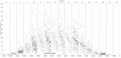
Fig. 3. Example of a forecast error scatter plot by time of the day (top x-axis) for 3-hours lead times and forecast error (y-axis)

compared between different forecast providers an evaluation of the “most costly errors” may reveal a very different result than, if only an average metric per forecaster would be used. By generating a framework of metrics, where forecast products are split up into their purpose and weighted with their individual measure for the overall performance value, complexity can be circumvented and a linear cost function can be established. Such frameworks are used in many busi-ness areas, for example in tender evaluations, where different types of qualification metrics are evaluated according to their importance to the organisation and the requirements. This can also mean that a forecast which is bought by one department in a company (e.g. operations) can be less than optimal in another department (e.g. trading).

It is therefore recommended to make a paradigm change and give the evaluation of forecast performance a level of attention that is equivalent to that assigned to the monitoring, process management and economic value assessment of the forecast. Moving towards such a paradigm shift, the following aspects should be taken into consideration in this process:

• Verification is subjective: It is important to understand

the limitations of a chosen metric

• Verification has an inherent uncertainty: The uncertainty

of verification results depends mainly on the size of the evaluation data set. When comparing forecasts, data sets need to be of exact same size to prevent random errors to supersede overall result.

• Evaluation should contain a selection of metrics:

– One metric alone does not provide the real perfor-mance of a forecast

– Use of de-compositions of errors explain the origin of errors. e.g. look at bias and variance alongside MAPE or RMSE.

– Selected metrics should reflect the costs of errors or security constraints to the greatest extent possible based on the user’s knowledge of the application’s characteristics

– Box plots and scatter plots reveal additional impor-tant information compared to a mean error metric

• Evaluation metric combinations can provide a represen-tative approximation of the “cost function”:

1) subjective evaluation through visual inspection 2) quantitative, dichotomous (yes/no) verification of

critical events such as high-speed shut-down or ramps with e.g. contingency tables

3) error ranges per important forecast horizon 4) error ranges per hour of day or forecast hour 5) error frequency distributions in ranges that have

different costs levels

6) separation of phase errors and amplitude errors according to their impact

7) parametric tests, bootstrapping can be used to look on individual error measures before averaging

IV. SUMMARY ANDOUTLOOK

In this paper, the outline and key points of the second and third parts of a IEA Wind Task 36 Recommended Practice guideline has been described. Conducting a trial or

benchmark requires attention to certain details in the design and execution phases otherwise disappointing results for the forecast providers and forecast user will be experienced. By following a 3-step procedure and considering a number of key points, the trial or benchmark effort will lead to significant results for implementing or renewing forecast services. Common pitfalls such as missing information, non-windy trial period, inconsistent data sets, can lead to inconsistent and non-representative results.

The guideline also discusses and recommends a paradigm shift in the evaluation of forecasts and forecast solutions. Single average metrics rarely provide the information about the value of the forecast for the user’s applications and often leads to misunderstandings and, at times, bad decisions in the selection process. Instead, it is recommended to work on establishing evaluation strategies with cost functions that reflect the costs associated with forecast errors and eventu-ally the value of a certain solution. A number of examples have been described to decompose errors in time ranges and size ranges that categorize the value or cost of errors of a certain type. Evaluation uncertainty and significance has been discussed in order to bring awareness to the fact that results, not considering the uncertainty and risks, can easily produce wrong results and lead to bad decisions. A statistical metric is only as useful as the significance of the error attributes that it was designed to measure and the consistency with which it is applied. In other words, if a metric is used in an inconsistent way, or does not measure the sensitivity of the user’s application to forecast error, the result does not provide meaningful information to the user’s process of selecting a forecast solution. The recommended practice guideline will provide detailed information on all these aspects and will be publicly available on the IEA Task homepage www.ieawindforecasting.dk.

ACKNOWLEDGMENT

The work of Corinna M¨ohrlen, Jakob W. Messner and Gregor Giebel is supported by the Danish EUDP project

IEA Wind Task 36 Forecasting Danish Consortium under

the contract no. 2015-II-499149. Jethro Browell is supported by an EPSRC Innovation Fellowship (EP/R023484/1). Data Statement: No new data were created during this study.

REFERENCES

[1] Madsen H., Pinson P., Kariniotakis G., Nielsen HA, Nielsen TS.,

Standardizing the Performance Evaluation of Short-Term Wind Power Prediction Models, Wind Engineering, 29(6), 475489. doi:10.1260/030952405776234599, 2005.

[2] Bessa RJ, Miranda V, Botterud A, Wang J, ’Good or bad wind power forecasts: a relative concept, Wind Energy, 14(5), 625636. doi:10.1002/we.444, 2010.

[3] Pinson P, Girard R, Evaluating the quality of scenarios of short-term wind power generation, Applied Energy, 96, 1220. doi:10.1016/j.apenergy.2011.11.004. Smart Grids, 2012.

[4] Diebold FX, Mariano RS, Comparing Predictive Accuracy, Journal of Business & Economic Statistics, 13(3), 253263. doi:10.1080/07350015.1995.10524599, 1995.

[5] Efron B, Nonparametric estimates of standard error: The jack-knife, the bootstrap and other methods, Biometrika, 68(3), 589599. doi:10.1093/biomet/68.3.589, 1981.

[6] Hamill, TM and Juras, J,Measuring forecast skill: is it real skill or is it the varying climatology?Q.J.R. Meteorol. Soc., 132: 2905-2923. doi:10.1256/qj.06.25, 2006.