Index based triangulation method for efficient generation of large three-dimensional ultrasonic C-scans

Index Based Triangulation method for efficient generation of

large three-dimensional ultrasonic C-scans

Carmelo Mineo, Jonathan Riise, Rahul Summan, Charles N. MacLeod, S. Gareth Pierce Department of Electronic and Electrical Engineering, University of Strathclyde

Royal College Building, 204 George Street, Glasgow G1 1XW, UK [email protected]

Abstract

The demand for high speed ultrasonic scanning of large and complex components is driven by a desire to reduce production bottlenecks during the non-destructive evaluation of critical parts. Emerging systems (including robotic inspection) allow the collection of large data volumes in short time spans, compared to existing inspection systems. To maximize throughput, it is crucial that the reconstructed inspection data sets are generated and evaluated rapidly without a loss of detail. This requires new data visualization and analysis tools capable of mapping complex geometries whilst guaranteeing full part coverage. This paper presents an entirely new approach for the visualization of three-dimensional ultrasonic C-scans, suitable for application to high data throughput ultrasonic phased array inspection of large and complex parts. Existing reconstruction approaches are discussed and compared with the new Index Based Triangulation (IBT) method presented. The IBT method produces 3D C-scan representation, presented as coloured tessellated surfaces, and the approach is shown to work efficiently even on challenging geometry. An additional differentiating characteristic of the IBT method is that it allows easy detection of lack of coverage (an essential feature to ensure that inspection coverage can be guaranteed on critical components). Results demonstrate that the IBT C-scan generation approach runs over 60 times faster than a C-scan display based on Delaunay triangulation and over 500 times faster than surface reconstruction C-scans.

In summary the main benefits of the new IBT technique are:

 High speed generation of C-scans on large ultrasonic data sets (orders of magnitude improvement over surface reconstruction C-Scans)

 Ability to operate efficiently on 3D mapped data sets (allowing 3D interpretation of C scans on complex geometry components)

 Intrinsic indication of lack of inspection coverage

Key words: C-scans; Phased arrays; Data visualisation; Robotics; Automated systems.

1. Introduction

1.1 Large scale ultrasonic scanning and current issues

demand projections (e.g. in the aerospace sector) and overcome the bottlenecks of safety critical NDT inspections, new automated scanning systems have been developed by a variety of research and development teams [1, 2]. Producing reliable automated solutions has become an industry priority to drive down inspection times and ensure repeatability. Applications of six-axis robotic arms in the NDT field have been recently published and there is a growing interest in using such automation solutions [3-7]. Modern robots used for automated NDT systems present precise mechanical joints and the ability to output their real-time pose at rates up to 1 kHz.

1.2 Types of data representations

Ultrasonic data can be collected and displayed in a number of different formats. Notoriously, the three common formats are known as A-scan, B-scan and C-scan presentations. The A-scan presentation displays the amount of received ultrasonic energy as a function of time or material depth (if the time is multiplied by the propagation speed of mechanical waves in the medium). B-scan presentations are profile (cross-sectional) views of the test specimen. In the B-scan, the time-of-flight (travel time) of the ultrasound energy (or the specimen depth) is displayed along the vertical axis and the linear position of the transducer is displayed along the horizontal axis. Typically, when it is necessary to test large specimens, a data collection gate is established on the A-scans and the amplitude or the time-of-flight of the ultrasound echoes is recorded at regular intervals as the transducer moves over the test piece. The measurements originating from this gating process, plotted in an X-Y plane using the acquisition locations of the A-scans, produce the C-scan presentations. The latter provide a feature map view of the position and size of specimen features. The plane of the image is parallel to the scan pattern of the transducer. The relative signal amplitude or the time-of-flight is displayed as a shade of grey or a colour map tint for each of the positions where data are recorded. The C-scan presentations provide an image of the features of the test piece that reflect and scatter the sound. These presentations have become by far the most common way ultrasonic data are visualized, since they allow screening the full extent of the specimen at once. When scanning highly curved surfaces, traditional C-scans images are typically shown as projections of the scanning trajectory on the X-Y plane. Since the three-dimensional nature of the specimen under inspection is lost in a bi-dimensional C-scan presentation, the sizing of the specimen features and the evaluation of the true relative distances between them can become very challenging. Evaluating the correct 3D distance between indications is crucial in applications where the standards impose limits on the defect density (number of defects per surface unit), besides on the maximum defect size [8].

A possible solution consists of partitioning large scans into small rectangular regions, where approximating the real surface geometry to a plane can be tolerated. Besides producing approximated sizing and measurements, this approach also complicates and slows down the data analysis process. This simplistic approach is not suitable for analysing the large data volumes that can be acquired at high speed through the integration of ultrasonic instrumentation and robotic manipulators. Robotic inspection systems currently under development will enable scanning large surfaces (e.g. a full aerospace wing) in a single pass, by streaming the ultrasonic data and the positional information to the hard disk of a dedicated data collection workstation [9].

examination of large NDT datasets [6, 9]. This work presents a new approach developed to revolutionise the visualization of three-dimensional C-scan maps based on a method of index triangulation. This paper explains the mathematical formulation of the new Index Based Triangulation technique. The advantages of the new approach are demonstrated and discussed.

2. Review of possible visualization approaches

Generating a three-dimensional C-scan map for curved surfaces is not a trivial task. This section presents a review of the visualization approaches available to date. The understanding of the existing methods is necessary to discuss the novelty aspects and the advantages of the new approach presented in this work.

2.1 Traditional 2D image presentation

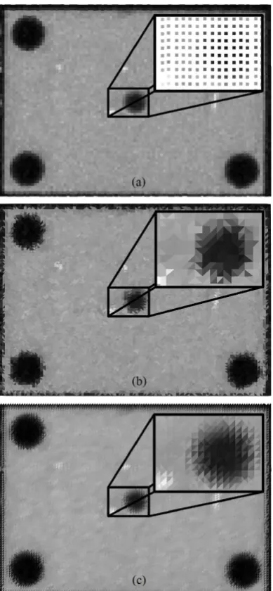
The traditional 2D presentation assumes the A-scans are collected at constant intervals and aligned in a rectangular grid. Therefore, the resulting C-scan image is an m-by-n grid of pixels where m is the number of columns and n is the number of rows. The X and Y coordinates of each A-scan acquisition location determine the centre of the corresponding pixel in the image. Given that the specimen is scanned at finite resolution and the A-scans are collected at fixed intervals, when a small section of the C-scan image is magnified, the small single-coloured square elements that comprise the image (pixels) become visible and the image is said to be pixelated. Figure 1 shows an ultrasonic scan of a 70x100mm steel plate using a KUKA KR5 robotic manipulator. The plate was scanned through a raster tool-path with the robot stopping at every 1mm interval along the x-direction and stepping by 1mm in the y-x-direction at the end of each scanning pass. An area of 11x15mm, magnified 2.5 times, is shown in the top right corner of the resulting traditional 2D C-scan map, (Figure 1c). The C-scan reveals the presence of an 8mm diameter flat bottom hole not visible from the top surface of the specimen. This example c-scan is used throughout the paper to illustrate the different visualization methods and the advantages of the novel approach.

Figure 1 – 70x100mm steel plate (a), scanned through a robotic arm (b). 2D C-scan image with a magnified area showing the pixelated nature of the data (c).

2.2 Coloured Point Cloud

An alternative way of displaying C-scan maps is as a point cloud with each point coloured according to the relative signal amplitude or the time-of-flight value originating from gated signal measurements. This visualization method allows using the raw point coordinates obtained directly from the manipulator encoders. Therefore, the robot can manipulate the probe through a continuous motion and A-scans can be acquired at variable intervals, since it is not necessary for the points to be exactly aligned according to a rectangular grid. The coloured point cloud display is intrinsically three-dimensional. This visualization approach was adopted by a software interface developed for a robotic inspection prototype system, which introduced the possibility of displaying 3D C-scans in 2015 [6].

the square sides or the circle diameters) can be specified equal to the spatial inspection resolution. On first inspection, this makes the point-cloud C-scan maps look like the traditional image-based C-scans. However, the data points are visually stacked in the order they were acquired; the fixed element size causes some points to overlap if their distance is lower than the average resolution value. Gaps can appear between adjacent elements that are a bit further from each other. The overlap increases when the display is zoomed out. The element separation increases when the C-scan map is magnified. This inconvenience can significantly hinder correct analysis of the inspection data. Figure 2a shows the point cloud based C-scan map relative to the same specimen mentioned previously. The magnified region shows the unwanted rarefaction of the points.

2.3 Tessellated Surfaces

The problem of overlapping points and rarefaction can be overcome by presenting the C-scan as a tessellated surface rather than a point cloud. Given the 3D C-C-scan data points, it is possible to use algorithms able to generate a mesh where each set of three close points become the vertices of one triangle. In a triangle mesh, the triangles are connected by their common edges or corners [11]. Therefore, a tessellated surface consists in triangles that fill the gaps between the data points. Since in the visualization of a tessellated surface the graphics engine does not need to turn the points into graphical objects on the screen the problem of overlapping points is removed. Tessellated surfaces are the workhorse of graphical engines and several visualization algorithms have been optimized for them (e.g. light ray intersection calculations, rendering, zooming, panning and 3D rotation) [12]; the same is not true for point cloud presentations, which need additional processing. The present work adopts triangulated meshes as a promising approach to handle and visualize large 3D C-scans, collected through modern robotised inspection systems.

There are two different ways to create a triangular tessellated surface from a point cloud: using triangulation methods or surface reconstruction methods. Triangulation algorithms use the original points of the input point cloud, using them as the vertices of the mesh triangles. Therefore, the colour given to the face of every triangle is extrapolated from the ultrasonic measurements associated to the triangle vertices. The Delaunay triangulation, named after Boris Delaunay for his work on the topic from 1934 [13], is the most popular algorithm of this kind. A 2-D Delaunay triangulation ensures that the circumcircle associated with each triangle contains no other point in its interior. This definition extends naturally to three dimensions considering spheres instead of circles. Figure 2b shows the C-scan map plotted through the Delaunay triangulation mesh.

Figure 2 – C-scan plotted as point cloud (a), Delaunay triangulation (b) and Poisson surface reconstruction (c).

3. New Index Based Triangulation (IBT) Approach

An intrinsic characteristic of the A-scans collected to create a C-scan map is the sequential way they are acquired along the scanning trajectory. The ultrasonic probe is moved along the predefined trajectory to cover the whole extent of the surface of interest and the A-scans are collected at regular intervals. The level of orderliness is even higher when the ultrasonic inspection is carried out through a phased array probe. The ordered spatial distribution of the A-scans locations, obtained through ultrasonic phased array probes, inspired the development of an efficient triangulation algorithm targeted to such structured point distribution.

𝑁 = {

𝑁𝑃−𝑁𝑆+1

𝑠 if (NP− NS) is odd 𝑁𝑃−𝑁𝑆

𝑠 + 1 if (NP− NS) is even

Eq. 1

where 𝑠 is the step in number of transducers between adjacent sub-aperture pulses. The distance between the locations encoding two consecutive A-scans of the frame is 𝑑 = 𝑠 ∙ 𝑝, where 𝑝 is the pitch of the phased array probe.

Phased Array Ultrasonic Testing (PAUT) of large surfaces is usually carried out using a raster tool-path. The probe is manipulated on a pass along the longitudinal direction of the specimen, covering a stripe of the surface. Then the probe is translated by a distance smaller than the stripe width for another pass over the surface. A small overlap is maintained between consecutive passes to ensure full NDT coverage.

In financial management and information technology, it has been observed that the lack of structure in databases makes both compilation and analysis time and energy-consuming tasks [16]. Whenever the information can be stored in the form of structured data with a high degree of organization, straightforward search engine algorithms or other search operations can be adopted. The ordered spatial distribution of the A-scans locations, obtained through ultrasonic phased array probes, inspired the development of an efficient triangulation algorithm targeted to such structured point distribution.

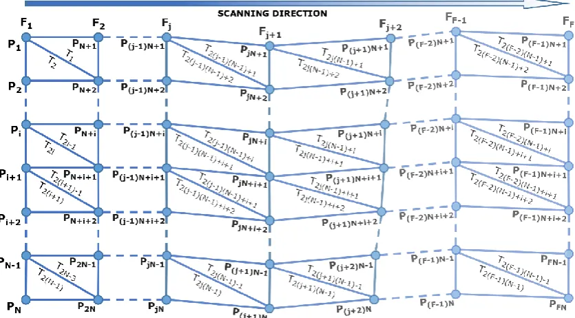
Given the number of A-scans contained in a frame (N) and the total number of frames (F), it is possible to create a table with the indices of the points to link, in order to create a neat and efficient triangulation. This approach is hereafter named as the Index Based Triangulation (IBT) algorithm. Assigning increasing indices to the points according to the electronic scanning direction within each frame and the mechanical scanning direction from frame 1 to frame F, the point indices span from 1 to [𝐹 ∙ 𝑁]. The indices of the points in the 𝑗th frame go from [(𝑗 − 1)𝑁 + 1] to [𝑗𝑁]. The index of the point relative to the 𝑖th pulse in the 𝑗th frame is [(𝑗 − 1)𝑁 + 𝑖].

Figure 3 – Scheme of indexes for the Index Based Triangulation (IBT) algorithm.

The points of the 𝑗th frame form 2(𝑁 − 1) triangles with the points of the (𝑗 + 1)th frame. From the first to the second-last point of the 𝑗th frame, each point is the vertex of two triangles. For example, the first and second frame produce the triangulation given in

Table 1. Each row of the table specifies a triangle, defined by indices with respect to the points. The triangulation between the jth and the (𝑗 + 1)th frame is given by a copy of Table 1, with all point indices incremented by (𝑗 − 1)𝑁. Therefore, the full triangulation for the C-scan can be expressed by a matrix (𝑻) representing the set of triangles that make up the triangulation.

Table 1 – Triangulation of the first two frames.

Tringles 1

st _vertex

index

2nd _vertex

index

3rd _vertex

index

T1 P1 PN+1 PN+2

T2 P1 PN+2 P2

T2i-1 Pi PN+i PN+i+1

T2i Pi PN+i+1 Pi+1

T2(i+1)-1 Pi+1 PN+i+1 PN+i+2

T2(i+1) Pi+1 PN+i+2 Pi+2

T2N-3 PN-1 P2N-1 P2N

T2(N-1) PN-1 P2N PN

The matrix is generated by appending (𝐹 − 1) copies of the 2(N-1) triangles in Table 1, were the values of each copy is incremented by the integer number [(𝑗 − 1)𝑁], with 𝑗 varying between 1 and (𝐹 − 1). The triangulation produces a meshed stripe whose length depends on the distance travelled by the probe and the width (w) is equal to:

𝑤 = (𝑁 − 1) ∙ 𝑝 Eq. 2

paused during the movement over an area without NDT interest (e.g. a hole in the specimen) or during the step movement at the end of each pass. If 𝑱 is the array of indices of the last frames acquired before such pauses, the unwanted triangles can be removed from 𝑻, by deleting the matrix rows between [2(𝑱 − 1)(𝑁 − 1) + 1] and [2𝑱(𝑵 − 1)].

Assuming 𝑛_𝐽 is the number of frame indices contained in 𝑱, the full triangulation matrix will have size of n-by-3, with n equal to:

𝑛 = 𝑛_𝑇− 2𝑛_𝐽(𝑁 − 1) Eq. 3

where, 𝑛_𝑇 is the total number of triangles initially created by the described index based triangulation, 𝑛_𝑇 = 2 ∙ (𝐹 − 1) ∙ (𝑁 − 1). The IBT based C-scan can be plotted in MATLAB®, through the function: 𝑡𝑟𝑖𝑠𝑢𝑟𝑓(𝑻, 𝑋, 𝑌, 𝑍, 𝐶). The function displays the triangles defined in the n-by-3 triangulation matrix 𝑻 as a surface. As described earlier, each row of 𝑻 contains indexes into the X, Y, and Z vertex vectors to define a single triangular face. The colour of the triangles is defined by the vector C. Since the IBT approach triangulates the original C-scan points, the vector C is the array of the original ultrasonic measurements collected from the gated A-scans.

The sample C-scan contains 7,550 points, acquired through a phased array probe with 𝑁_𝑃 = 32, 𝑁_𝑆 = 8, 𝑠 = 1 and 𝑝 = 1mm. With such parameters, the height of the plate surface in Figure 1 is covered by three inspection raster scan passes with width (𝑤) equal to 24mm, overlapping by 1mm. Figure 4 shows the C-scan map obtained through the application of the IBT algorithm to such rearranged point cloud distribution. The 7x magnification of the central areas illustrates how the IBT C-scan looks similar to the pixelated image-based C-scan in Figure 1, with the advantage that the triangular mesh uses the original A-scan locations as triangle vertices.

4. Quantitative performance results

Up to this point, the sample C-scan introduced in Figure 1 has been used to explain the theoretical background of the IBT method and discuss its features. Two additional C-scan datasets were acquired through a robotic phased array inspection system. All C-scans were used to compare the computational efficiency of the IBT method with the Delaunay triangulation and the Poisson’s algorithm quantitatively. The second obtained C-scan contains 793,572 A-scan points and the third C-scan over 2.7 million points.

The three algorithms were tested, using a computing machine based on an Intel® Core(TM) i7-6820HQ CPU (2.70GHz), with 32Gb of RAM. The benchmarking was carried out through MATLAB® 2016a, running on the Windows 10 64-bit operating system. The inbuilt MATLAB® function, 𝑻 = 𝑑𝑒𝑙𝑎𝑢𝑛𝑎𝑦(𝑋, 𝑌), was used to test the Delaunay triangulation. This function produces good results only when the input points are distributed on a surface that can be mathematically described by a surjective function in the X-Y domain. The 3D version of Delaunay triangulation, 𝑻 = 𝑑𝑒𝑙𝑎𝑢𝑛𝑎𝑦(𝑋, 𝑌, 𝑍), is able to operate with non-surjective surfaced, as long as they are closed surfaces and three-dimensionally convex. These constraints make the 3D Delaunay function of no utility in our case, so the 2D Delaunay function was used. The Poisson’s surface reconstruction algorithm of M. Kazhdan [15], coded in C++ programming language and compiled as a MATLAB® MEX-File, was used to test the Poisson’s method. The IBT approach, described in Section 3, was implemented in a MATLAB® function by the authors of the present work.

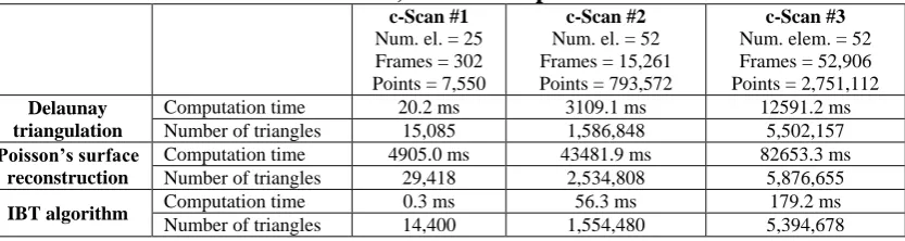
Table 2 reports the results of the benchmarking tests.

The Poisson’s formulation generated the highest number of triangles for all datasets. This was expected, since this approach extends the reconstructed surface beyond the boundary of the original point cloud. Moreover, the new vertex points generated by the Poisson’s method required interpolating of the ultrasonic measurements associated to the original points. Besides altering the original spatial sampling resolution of the original point cloud, the surface reconstruction method revealed to be the most time-consuming approach, requiring over 80 seconds for the largest dataset.

The Delaunay triangulation is faster than the surface reconstruction and produces a smaller number of triangles. The method required 12.6 seconds for the largest dataset. The new IBT approach generated the smallest number of triangles for all datasets. The method creates simple meshed stripes of triangulated frame points. Stripes belonging to consecutive passes are not sown together by stitching triangles. The triangles connecting consecutive frames that are far from each other are removed from the triangulation, allowing the presence of concave regions in the 3D C-scan map. The IBT algorithm was by far the fastest, with computation times of 0.3ms, 56.3ms and 179.2ms, respectively for the smallest, medium and largest dataset. The IBT method shows enhanced performance because the triangulation algorithm requires only the construction of a matrix of indices. The processor performs simple algebraic operations on integers, rather than double precision numbers. The implementation of the IBT algorithm was based on the uint32

Table 2 – Performance of Delaunay triangulation, Poisson’s surface reconstruction and IBT method, for three input datasets.

c-Scan #1

Num. el. = 25 Frames = 302 Points = 7,550

c-Scan #2

Num. el. = 52 Frames = 15,261 Points = 793,572

c-Scan #3

Num. elem. = 52 Frames = 52,906 Points = 2,751,112

Delaunay triangulation

Computation time 20.2 ms 3109.1 ms 12591.2 ms Number of triangles 15,085 1,586,848 5,502,157

Poisson’s surface reconstruction

Computation time 4905.0 ms 43481.9 ms 82653.3 ms Number of triangles 29,418 2,534,808 5,876,655

IBT algorithm Computation time 0.3 ms 56.3 ms 179.2 ms

Number of triangles 14,400 1,554,480 5,394,678

5. Discussion of additional benefits

The Delaunay triangulation and the Poisson’s surface reconstruction algorithm stitch the mesh triangles belonging to consecutive passes together. The stitching of consecutive passes is problematic, since a too large raster step (the distance the probe is translated by at the end of each pass) may not appear as an evident gap in the C-scan map during the data analysis phase. This stitching results in closing gaps, which would otherwise be evident resulting in a lack of coverage going unnoticed by the NDT inspector. The IBT algorithm does not create stitching triangles between the raster scan passes constituting the C-scan map. Therefore, a lack of NDT coverage can easily be found.

5.2 Coherent triangle normals

Graphic engines simulate a certain flux of light in 3D plots. The mesh triangles are illuminated differently according to the angle at which the light arrives to them. Therefore, the colour that graphic engines assign to each triangle is strongly affected by the normal to the triangle surface. The normal of a triangle is computed by taking the cross product of two of its edges. Reversing the order of the triangle vertices flips the direction of the triangle normal. The Delaunay triangulation and the Poisson’s surface reconstruction are unable to maintain a consistent direction in the linkage of the triangle vertices. This has an undesired effect on the colouring of the resulting C-scan maps (see Figure 2b and Figure 2c). The IBT algorithm ensures that all triangle vertices are connected clockwise, producing coherent normals and colouring.

5.3 Concave and convex shapes

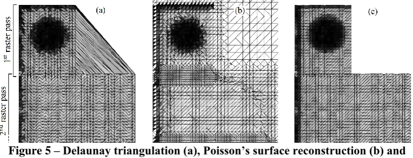
Surfaces can have convex and concave areas. In a convex shape, a line segment between any two points within the shape always falls completely inside the shape. However, for a concave (or non-convex) shape, the same is not true for all possible line segments connecting points on the shape. If at least one-line segment falls outside of the shape, then the shape is concave. The Delaunay triangulation is only suitable for triangulating convex surfaces. Indeed, the problem of finding the Delaunay triangulation of a set of points can be converted to the problem of finding the convex hull of the set [17]. This is an enormous inconvenience in the generation of tessellated surfaces for C-scan presentations.

Poisson’s surface reconstruction method (see Figure 5b). In this case, the generation of unwanted triangles arises because the Poisson’s algorithm does not follow the boundary of the point cloud and replaces the original points with new points laying on a reconstructed continuous surface, satisfying the Poisson’s differential equation. The size of the triangles increases outside the region containing the original points.

The IBT algorithm manages to produce the expected results, generating a meshed surface stripe, with no redundant or unwanted triangles (see Figure 5c). The new approach appears to be extremely advantageous over other methods, to generate C-scan representations for shapes with concave regions.

Figure 5 – Delaunay triangulation (a), Poisson’s surface reconstruction (b) and IBT based C-scan (c), for a concave shape.

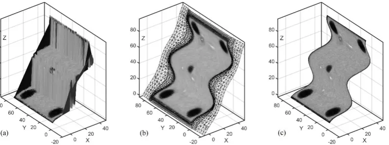
5.4 Highly curved geometries

The sample C-scan presented above is parallel to the plane of the steel plate surface. To illustrate how the IBT algorithm handles highly complex surfaces, the original Cartesian positional data was modified. The Z-coordinate of the C-scan points has been replaced with a sinusoidal pattern, to simulate the challenges of a curved geometry. Moreover, the resulting 3D point cloud has been rotated by 60 degrees around the Y-axis.

Figure 6 – Delaunay triangulation (a), Poisson surface reconstruction (b) and IBT based C-scan (c), for a challenging 3D shape with non-surjective regions.

6. Conclusions

This paper presented a new approach for the generation of three-dimensional ultrasonic C-scans of large and complex parts increasingly encountered in manufacturing. New data visualization and data analysis tools, suitable to screen the NDT information obtained through high speed inspection systems, are urgently required to decrease the time needed for data analysis. The novel Index Based Triangulation (IBT) method was introduced and described. In summary the main benefits of the new IBT technique are:

 High speed generation of C scans on large ultrasonic data sets (orders of magnitude improvement over surface reconstruction C Scans);

 Ability to operate efficiently on 3D mapped data sets (allowing 3D interpretation of C scans on complex geometry components);

 Intrinsic indication of lack of inspection coverage.

The approach is applicable to ultrasonic data gathered in a structured and orderly fashion such as that obtained from ultrasonic phased array probes. The method produces 3D C-scans, presented as coloured tessellated surfaces using an indexing method. The approach works efficiently on challenging geometries incorporating concave and convex regions, and allows easy detection of lack of coverage. Whilst this has been illustrated in the paper through geometric distortion of simple sample data sets, note that the technique has been tested by the authors on complex geometries in composite and metallic specimens (that are commercially sensitive and cannot be directly placed in the public domain). It is envisaged that the presented method can be further researched, applied and utilised in emerging data visualization tools for robotic/automated ultrasonic inspection systems.

Qualitative and quantitative results have been presented. The IBT C-scan generation resulted over 60 times faster than C-scan display based on Delaunay triangulation and over 500 times faster than C-scans based on Poisson’s surface reconstruction meshes. The method is potentially extensible to other ordered data sets, for example in laser-based geometry mapping of curved surfaces.

Acknowledgements

References

[1] C. N. MacLeod, S. G. Pierce, M. Morozov, R. Summan, G. Dobie, P.

McCubbin, et al., "Automated metrology and NDE measurements for increased throughput in aerospace component manufacture," in 41st annual review of progress in Quantitative Nondestructive Evaluation, 2015, pp. 1958-1966. [2] T. Sattar, "Robotic non-destructive testing," Industrial Robot: An International

Journal, vol. 37, 2010.

[3] F. Bentouhami, B. Campagne, E. Cuevas, T. Drake, M. Dubois, T. Fraslin, et al., "LUCIE - A flexible and powerful Laser Ultrasonic system for inspection of large CFRP components.," presented at the 2nd International Symposium on Laser Ultrasonics, Talence (France), 2010.

[4] A. Maurer, W. D. Odorico, R. Huber, and T. Laffont, "Aerospace composite testing solutions using industrial robots," presented at the 18th World

Conference on Nondestructive Testing, Durban, South Africa, 2012. [5] J. T. Stetson and W. D. Odorico, "Robotic inspection of fiber reinforced

aerospace composites using phased array UT," presented at the 40th Annual Review of Progress in Quantitative NDE, Baltimore, Maryland, 2013.

[6] C. Mineo, S. Pierce, B. Wright, I. Cooper, and P. Nicholson, "PAUT inspection of complex-shaped composite materials through six DOFs robotic

manipulators," Insight-Non-Destructive Testing and Condition Monitoring, vol. 57, pp. 161-166, 2015.

[7] E. Cuevas, S. Hernandez, and E. Cabellos, "Robot-Based Solutions for NDT Inspections: Integration of Laser Ultrasonics and Air Coupled Ultrasounds for Aeronautical Components," in 25th ASNT Research Symposium, 2016, pp. 39-46.

[8] W. A. Levinson, "Control Charts Control Multiple Attributes," Quality, vol. 43, p. 40, 2004.

[9] C. Mineo, C. MacLeod, M. Morozov, S. G. Pierce, T. Lardner, R. Summan, et al., "Fast ultrasonic phased array inspection of complex geometries delivered through robotic manipulators and high speed data acquisition instrumentation," in Ultrasonics Symposium (IUS), 2016 IEEE International, 2016, pp. 1-4.

[10] H. Pfister, M. Zwicker, J. Van Baar, and M. Gross, "Surfels: Surface elements as rendering primitives," in Proceedings of the 27th annual conference on

Computer graphics and interactive techniques, 2000, pp. 335-342. [11] M. Botsch, L. Kobbelt, M. Pauly, P. Alliez, and B. Lévy, Polygon mesh

processing: CRC press, 2010.

[12] I. Wald and V. Havran, "On building fast kd-trees for ray tracing, and on doing that in O (N log N)," in 2006 IEEE Symposium on Interactive Ray Tracing, 2006, pp. 61-69.

[13] B. Delaunay, "Sur la sphere vide," Izv. Akad. Nauk SSSR, Otdelenie Matematicheskii i Estestvennyka Nauk, vol. 7, pp. 1-2, 1934.

[14] F. Calakli and G. Taubin, "SSD: Smooth signed distance surface reconstruction," in Computer Graphics Forum, 2011, pp. 1993-2002.

[16] H. Baars and H.-G. Kemper, "Management support with structured and

unstructured data—an integrated business intelligence framework," Information Systems Management, vol. 25, pp. 132-148, 2008.

[17] M. De Berg, M. Van Kreveld, M. Overmars, and O. C. Schwarzkopf,