A Simulation Based Optimization Approach for Stochastic Resource Constrained Project Management with Milestones

Rochester Institute of Technology

RIT Scholar Works

Theses Thesis/Dissertation Collections

8-2015

A Simulation Based Optimization Approach for

Stochastic Resource Constrained Project

Management with Milestones

Maribel Perez

Follow this and additional works at:http://scholarworks.rit.edu/theses

This Thesis is brought to you for free and open access by the Thesis/Dissertation Collections at RIT Scholar Works. It has been accepted for inclusion in Theses by an authorized administrator of RIT Scholar Works. For more information, please [email protected].

Recommended Citation

Rochester Institute of Technology

A SIMULATION BASED OPTIMIZATION APPROACH FOR STOCHASTIC

RESOURCE CONSTRAINED PROJECT MANAGEMENT WITH MILESTONES

A Thesis

Submitted in partial fulfillment of the requirements for the degree of

Master of Science in Industrial & Systems Engineering

in the

Department of Industrial & Systems Engineering

Kate Gleason College of Engineering

by Maribel Perez

i

DEPARTMENT OF INDUSTRIAL AND SYSTEMS ENGINEERING

KATE GLEASON COLLEGE OF ENGINEERING

ROCHESTER INSTITUTE OF TECHNOLOGY

ROCHESTER, NEW YORK

CERTIFICATE OF APPROVAL

M.S. DEGREE THESIS

The M.S. Degree Thesis of Maribel Perez

has been examined and approved by the

thesis committee as satisfactory for the

thesis requirement for the

Master of Science degree

Approved by:

____________________________________ Dr. Michael E. Kuhl, Thesis Advisor

ii

ABSTRACT

Project managers are challenged to continuously make decisions throughout the

development of a project attempting to minimize the overall project cost and, at the same time,

seeking to accomplish a pre-established deadline. These time-cost tradeoff decisions are made

even more complex when resource constraints, caused by limited available resources, are added

to the equation. The goal of this research is to design a simulation-based optimization approach

to solve the resource constrained project scheduling problem (RCPSP) under uncertainty. Two

methods are proposed: the Total Cost Resource Constrained Method (TCRCM) and the Earned

Value Resource Constrained Method (EVRCM). The TCRCM seeks to minimize the total

project cost, including activity and penalty costs due to lateness at project completion, while

considering the RCPSP with stochastic activity times and costs in terms of resource alternatives

as well as precedence relationships for activities sharing resources. The EVRCM, which is based

on earned value management, not only considers penalty costs at project completion, but at

several project milestones along the execution of the project. Both methods can be implemented

in two phases: Phase I, and Phase II. Phase I is implemented prior the start of the project to

determine the optimal resource configuration for the entire project based on the specified

performance measure (e.g. total project cost). Phase II is implemented as the project progresses

to determine the optimal resource configuration for the remaining activities of the project. The

robustness of both methods is evaluated through a set of experiments. Lastly, the methods are

iii

TABLE OF CONTENTS

ABSTRACT ... ii

1 INTRODUCTION... 1

2 PROBLEM STATEMENT ... 4

3 LITERATURE REVIEW ... 7

3.1 Project Scheduling Techniques ... 7

3.2 Resource Constrained Project Scheduling Problem (RCPSP) ... 11

3.3 Simulation Optimization ... 15

3.4 Earned Value Management Terminology ... 17

3.4.1 Earned Value Main Components ... 18

3.4.2 Earned Value Performance Measures ... 19

3.4.3 Earned Value Forecasting Indicators ... 21

3.5 Discussion ... 23

4 TOTAL COST RESOURCE CONSTRAINED METHOD FOR RCPSP BASED ON EXPECTED TOTAL PROJECT COST ... 25

4.1 Overview of the Simulation-Based Optimization Approach ... 28

4.1.1 Assumptions ... 29

4.1.2 TCRCM: Input Parameters ... 30

4.1.3 TCRCM: Optimization Model ... 31

4.1.4 TCRCM: Simulation Model ... 35

4.1.5 TCRCM: Output Parameters... 39

4.1.6 TCRCM: Project Simulator ... 39

4.2 TCRCM: Implementation ... 40

4.3 TCRCM: Applied Prior the Start of the Project... 44

4.4 TCRCM: Phase I Example... 46

4.5 TCRCM: Applied During Project Execution ... 51

4.6 TCRCM: Phase II Example ... 53

4.7 TCRCM: Experiments ... 62

4.7.1 Experimental Case 1 ... 65

4.7.2 Experimental Case 2 ... 71

4.7.3 Experimental Case 3 ... 76

4.7.4 TCRCM: Experimental Cases Discussion ... 81

4.8 Summary of TCRCM ... 82

5 EARNED VALUE RESOURCE CONSTRAINED METHOD BASED ON MULTIPLE PROJECT MILESTONES ... 83

5.1 EVRCM: Applied Prior the Start of the Project ... 88

5.1.1 EVRCM: Phase I Assumptions ... 90

5.1.2 EVRCM: Phase I Input Parameters ... 90

5.1.3 EVRCM: Phase I Optimization Model ... 91

iv

5.1.5 EVRCM: Phase I Output Parameters ... 94

5.1.6 EVRCM: Phase I Project Simulator ... 96

5.1.7 EVRCM: Phase I Implementation ... 96

5.1.8 EVRCM Applied to the Selection of Resource Alternatives: Phase I Example ... 99

5.1.9 EVRCM Applied to the RCPSP: Phase I Example ... 107

5.2 EVRCM: Applied During Project Execution ... 115

5.2.1 EVRCM: Phase II Assumptions ... 117

5.2.2 EVRCM: Phase II Input Parameters ... 117

5.2.3 EVRCM: Phase II Optimization Model ... 117

5.2.4 EVRCM: Phase II Simulation Model ... 120

5.2.5 EVRCM: Phase II Output Parameters ... 122

5.2.6 EVRCM: Phase II Project Simulator ... 122

5.2.7 EVRCM: Phase II Implementation ... 123

5.2.8 EVRCM Applied to the Selection of Resource Alternatives: Phase II Example ... 126

5.2.9 EVRCM Applied to the RCPSP: Phase II Example ... 137

5.3 EVRCM: Experiments ... 146

5.3.1 EVRCM for Resource Alternatives: Experiments ... 147

5.3.2 EVRCM for RCPSP: Experiments ... 169

5.4 Summary of EVRCM ... 191

6 MS EXCEL USER INTERFACE... 192

6.1 TCRCM User Interface ... 193

6.2 EVRCM User Interface... 202

7 CONCLUSIONS & RECOMMENDATIONS FOR FUTURE RESEARCH ... 215

7.1 TCRCM Conclusions ... 215

7.2 EVRCM Conclusions... 216

7.3 Recommendations for Future Work... 217

REFERENCES ... 218

APPENDICES ... 221

Appendix A. Example of the Implemented TCRCM ... 221

Appendix B. Industrial Strength COMPASS (ISC) Input Parameters ... 229

Appendix C. Input Files ... 231

Appendix D. TCRCM Template User Manual ... 252

1

1

INTRODUCTION

Project management is the application of knowledge, skills, tools, and techniques to

project activities to meet the project requirements (PMI, 2008). Project management is all about

administering and "balancing the competing project constraints, which include, but are not

limited to: scope, quality, schedule, budget, resources and risks" (PMI, 2008), in order to

complete a project on time, budget, and scope.

In the early planning stages of a project, an effort is made to identify the main activities

of the project as well as their precedence relationship, estimated duration, and associated costs.

As the next step, resources are assigned to the project tasks. Assigning different resources to all

activities of the project would certainly make resource allocation simple and provide the shortest

project completion time. However, that approach is not guaranteed to minimize project cost.

Furthermore, in reality, project managers need to face not only resource scarcity, but also the

lack of skilled resources that would qualify to perform a particular activity. Commonly,

resources capabilities are limited by their expertise and knowledge on how to perform the task.

Hence, resource availability is not only dependent on the current number of resources but also

the skills of potential resources.

Throughout this research, the resource constrained project scheduling problem (RCPSP)

under uncertainty is investigated. The RCPSP consists of the allocation of resources to

competing activities in an efficient way (Bhaskar, Pal & Pal, 2011). In the proposed method, the

RCPSP is approached by selecting from among potential resource alternatives with associated

stochastic durations and costs, while simultaneously considering precedence decisions for

2

assignment and resource precedence, with the purpose of minimizing project cost at project

milestones.

To better explain the problem, a sample project network is shown in Figure 1.1. In this

network, the numbered nodes represent the activities of the project (in this case there are a total

of 12 activities) and the nodes labeled “S” and “F” represent the start and finish of the project.

The letters above each node represent the potential resource alternatives that could execute that

task. The solid arcs symbolize the precedence relationships between activities and the dashed

arcs represent the potential precedence constraints if the same resource was chosen to execute

both activities. For example, if resource D was selected to perform both activities 5 and 6, the arc

direction would need to be determined and, afterwards, a resource precedence relationship would

be imposed between the activities. Given multiple potential configurations to select from, finding

the optimal resource configuration for a network, such as the one shown, could get very

complex.

3

This research presents a simulation-based optimization approach that focuses on

identifying the optimal scheduling scheme that minimizes the cost of the project. The method

consists of two phases. The Static Phase, which is executed before the project begins, determines

the best resource configuration based on potential resource alternatives with associated stochastic

times and costs. The Dynamic Phase, which is implemented during project execution,

reevaluates resource configurations for the remaining activities of the project considering that the

uncertainty associated with completed and in progress activities is eliminated.

The rest of this thesis is structured as follows. Chapter 2 presents the problem statement

and the fundamental objectives of this research. Chapter 3 includes a review of the current

literature with regard to project scheduling techniques, resource constrained project scheduling

problem (RCPSP), simulation optimization, and earned value management. Chapter 4 presents

the proposed scope and methodology for the Total Cost Resource Constrained Method

(TCRCM). Chapter 5 presents the proposed scope and methodology for the Earned Value

Resource Constrained Method (EVRCM). Chapter 6 presents the MS Excel user interface

developed for the TCRCM and the EVRCM. Chapter 7 presents the conclusions drawn from this

4

2

PROBLEM STATEMENT

Given the complexity of scheduling resources while attempting to obtain the optimal

project cost at project milestones, the goal of this research is to develop a tool that provides

project managers information regarding the optimal resource scheduling scheme for their

projects. A simulation-based optimization approach that evaluates different resource

configurations for project activities considering their associated stochastic times and costs, as

well as penalty costs due to tardiness, is investigated. Two methods, which are both based on a

simulation-based optimization approach, are developed in this research:

 Total Cost Resource Constrained Method (TCRCM): This method seeks to identify the

optimal resource configuration for the RCPSP in terms of resource assignments and

resource precedence relationships by minimizing the total expected project cost at a

single project milestone (project completion).

 Earned Value Resource Constrained Method (EVRCM): This method, which is based on

earned value management, seeks to identify the optimal resource configuration that

minimizes the expected cost of the project, which consists of activity costs and lateness

penalty at several project milestones. This method is applied to two problems: 1)

Selection of Resource Alternatives, and 2) the RCPSP.

The main objectives of this research are to:

 Develop a simulation-based optimization method for stochastic resource constrained

project management with a single project milestone: In order to solve the resource

constrained problem, there are two main questions that need to be answered. First, for

5

alternative needs to be selected for each project activity. Additionally, for activities

sharing resources, the order of activity execution has to be determined. The method

should be able to provide the optimal resource configuration that minimizes project cost

during the static phase (Phase I), that is, prior the start of the project. In addition, the

method should be capable of reevaluating the project along its progression in order to

provide the optimal resource configuration from that point forward by only considering

uncertainty of activities that have not been started.

 Develop a simulation-based optimization method based on Earned Value Management

for stochastic resource constrained project management with several project milestones:

Design a method that uses earned value management to determine the optimal resource

configuration by not only considering penalties associated with lateness at project

completion but also at several project milestones along the execution of the project. The

method is to be applied to the selection of resource alternatives as well as the RCPSP in

terms of resource alternatives with associated stochastic times and costs and resource

precedence relationships. The method should be able to provide the optimal resource

configuration that minimizes planned value during the Static phase (Phase I), that is, prior

the start of the project. In addition, the method should be capable of reevaluating the

project along its progression in order to provide the optimal resource configuration for

6

 Conduct an experimental performance evaluation: The capabilities and limitations of the

proposed tool will be evaluated through experimentation. A set of experimental cases will

be used to evaluate the TCRCM. These cases are characterized by a range of

complexities including varying resource alternatives, resource precedence relationships,

levels of variability in activity costs and times, and penalty functions. The EVRCM will

be applied to two problems: 1) Selection of resource alternatives, and 2) The RCPSP.

Cases are utilized to evaluate each problem. When applying the EVRCM to the first

problem, cases with varying resource alternatives, levels of variability, number of project

milestones and weighted penalty functions will be considered. For the EVRCM applied

to the RCPSP, in addition to the complexities mentioned for the TCRCM, multiple

project milestones and weighted penalty functions will be evaluated. For each method,

the experimental evaluation will be conducted for the static and dynamic phase.

 Integrate the proposed optimization method with Microsoft Excel: With the purpose of

making the use of the proposed methods as user friendly as possible, the TCRCM and

EVRCM are both integrated to Microsoft Excel. The user will be able to input basic

information associated with the project under evaluation and easily run the

simulation-based optimization methods. The optimal solution will be imported automatically to the

Excel workbook as well as the Earned Value Graphs (for EVRCM) by simply clicking a

button.

By developing the simulation-based optimization methods, a more efficient resource

schedule that minimizes expected project cost under uncertainty will be generated, aiding project

7

3

LITERATURE REVIEW

The current chapter presents a synopsis of the concepts and terms related to this research.

These concepts and terms include project scheduling techniques, the resource constrained project

scheduling problem (RCPSP), simulation optimization, and earned value management

terminology. At the end of the chapter, the contribution provided by this research to the existing

literature will be discussed.

3.1

Project Scheduling Techniques

Scheduling refers to creating a defined plan for a project which clearly indicates the start

and end of project activities. (Vanhoucke, 2012). Scheduling complexities due to constraints

imposed by the characteristics of a project have accelerated the study of methods that simplify

the planning phase efforts. Scheduling techniques in project management began with the

development of the Gantt chart by Henry Gantt; technique that serves as platform for two

scheduling methods developed later on (Vanhoucke, 2012). Critical Path Method (CPM) and

Project Evaluation and Review Technique (PERT) have been widely used since the 1950s as

project scheduling techniques. CPM was developed in 1957 with the purpose of utilizing a

computer in scheduling construction programs, so that such programs could be completed on

time and within cost estimates (Wolf & Hauck, 1985). PERT was implemented in 1958 by the

U.S. Navy for managing the development of the Polaris missile program (Wolf & Hauck, 1985).

Although CPM and PERT were developed independently, they share certain similarities such as

the critical path calculations which serve as a basis for both. These calculations revolve around

identifying the longest path of the project network. That is, the critical activities which cannot be

delayed without extending the project completion time. In addition, the total slack of the project

8

task can be delayed without impacting the project duration is known. To calculate the critical

path, the following parameters need to be calculated (Kerzner, 2013):

1. Earliest start time (ES) and earliest finish time (EF) can be calculated during the forward

pass. Going through the network from left to right, the earliest starting time of a

successor activity is the latest of the earliest finish times of the predecessors. The earliest

finish is the addition of the earliest starting time and the activity duration.

2. Latest start time (LS) and Latest finish time (LF) are calculated during the backward pass

through the network. Since the activity time is known, the latest starting time can be

determined by subtracting the activity time from the latest finishing time. The latest

finishing time for an activity entering the node is the earliest starting time of the activities

exiting the node.

3. Slack time is determined after the forward and backward passes have been completed.

The slack is equal to the latest finish time minus the earliest finish time.

Several characteristics that are essential for analysis by CPM or PERT include (Wiest &

Levy, 1977):

 The project consists of a well-defined collection of jobs, or activities, which when

completed mark the end of the project.

 The jobs may be started and stopped independently of each other, within a given

sequence.

 The jobs are ordered; that is, they must be performed in technological sequence.

Despite their similarities, CPM and PERT differ in numerous ways. CPM is basically

concerned with obtaining the trade-off between cost and completion date for large projects; it

9

in a project and the cost of these resources (Wiest & Levy, 1977). CPM does not manage

uncertainty in activity durations, in fact, the completion time of each activity is known with

certainty. On the other hand, PERT was implemented to cope with the uncertainties identified

during the managing of a development program. PERT has proven to be a useful tool in planning

and scheduling large projects which consist of numerous activities whose completion times are

uncertain (Wiest & Levy, 1977). Hence, PERT is used more in research and development

projects where probabilistic times are used for activity duration, and CPM is used more in

projects such as construction, where there has been some experience in handling similar

endeavors and activity times can be estimated more accurately (Wiest & Levy, 1977). Other

ways in which these two techniques differ are in that CPM is “built up from jobs (or activities)

instead of events” (Battersby, 1970), and that it relates times to costs.

Some of the assumptions underlying CPM and PERT include (Wiest & Levy, 1977):

 A project can be subdivided into a set of predictable, independent activities.

 The precedence relationships of project activities can be completely represented by a

noncyclical network graph in which each activity connects directly into its immediate

successors.

 Activity times may be estimated – either as single-point estimates or as three-point PERT

estimates – and are independent of each other.

Although some of these assumptions are true for realistic scheduling problems, the

assumption of independence of activity durations is not aligned with situations observed in

practice. Resource limitations may cause time dependencies of activities sharing the same

resources (Wiest, & Levy, 1977); for an activity to begin, all technical and resource

10

resource that will execute the activity must be available. Hence, scheduling one activity may

cause another independent activity to be stretched out (or postponed) because of a lack of

sufficient common resources (Wiest & Levy, 1977). For this reason the basic time-only

PERT/CPM forward-backward pass procedure has been called by some seasoned users, a

feasible procedure for producing nonfeasible schedules (Moder, Phillips & Davis, 1983). When

considering resource constraints in PERT/CPM, the following is true (Moder, Phillips & Davis,

1983):

 Resource constraints reduce the total amount of schedule slack.

 Slack depends both upon activity precedence relationships, and resource limitations.

 The early and late start schedules are typically not unique since they depend upon the

scheduling rules used for resolving resource conflicts.

 The critical path in a resource-constrained schedule may not be the same continuous

chain(s) of activities as occurring in the unlimited resources schedule.

Given the limited capabilities of PERT/CPM to manage resource constraints, other

scheduling procedures are used for this purpose. Scheduling procedures for dealing with resource

constraints can be roughly divided into 2 major groups, according to the problem addressed

(Moder, Phillips & Davis, 1983):

 Resource Leveling: occurs when sufficient total resources are available, and the project

must be completed by a specified due date, but it is desirable or necessary to reduce the

amount of variability in the pattern of resource usage over the project duration.

 Fixed Resource Limits Scheduling: This category of problem, which is much more

11

out the project. The scheduling objective in this case is to meet project due dates insofar

as possible, subject to the fixed limits on resource availability.

Heuristic approaches have been used to improve the PERT/CPM procedures when

dealing with resource constraints. Kim & Garza (2003) proposed a step-by-step

resource-constrained path method (RCPM) that not only considered technical precedence constraints for

CPM calculations in the forward and backward pass process, but also accounted for

resource-constrained relationships. Hence, unlike CPM, the critical path identified through the RCPM

would be representative of the resource constrained network. Lu & Lam (2008) investigated “the

current practice of CPM scheduling under resource limit and calendar constraints” by evaluating

the P3 software tool. Lu & Lam (2008) proposed a method for calculating activity total float

during the forward pass analysis of the CPM method while considering resource calendar

restrictions. The results of the method were compared to the results produced by P3 in order to

identify any limitations of the software.

3.2

Resource Constrained Project Scheduling Problem (RCPSP)

The lack of skilled resources to allow the simultaneous execution of activities is a

problem project managers face regularly. Limited resources impose a whole new set of

constraints to the scheduler: job start times are constrained not only by precedence relationships

but also by resource availabilities (Wiest & Levy, 1977). The absence of available resources with

the required set of skills necessary to execute a project task can impact the project schedule

and/or project total cost. Therefore, scheduling resources while considering time-cost tradeoffs

can be a very challenging and complex task. The Resource Constrained Project Scheduling

Problem (RCPSP) is a well-researched problem, which involves allocating scarce resources to

12

some activities over time such that scarce resource capacities are respected and a certain

objective function is optimized (Brucker & Knust, 2011).

Due to the complexities of such a problem, various heuristic-based approaches have been

developed to solve the RCPSP. Kelley (1963), who first introduced the RCPSP, proposed and

applied two heuristic scheduling techniques with the purpose of minimizing total cost: parallel

and serial scheduling methods. In both methods, the set of schedulable activities are identified

and a priority rule is used to define which activities will be scheduled considering limited

resources. In parallel scheduling, all activities starting in a given time period are ranked as a

group in order of priority and resources are allocated according to this priority as long as

available (Moder, Phillips & Davis, 1983). On the other hand, in serial scheduling, “all activities

of the project are ranked in order of priority as a single group, using some heuristic, and then

scheduled one at a time” (Moder, Phillips & Davis, 1983). Gordon (1983) published a

comparison between the serial and the parallel method concluding that the serial procedure gives

better results for some categories of project networks than the parallel procedure. Despite this

and the fact that the parallel method requires more computing time, the parallel method “appears

to be more widely used than the serial method” (Moder, Phillips & Davis, 1983).

Wiest (1966) proposed a simple heuristic program based on three priority rules:

 Allocate resources serially in time; that is, schedule all activities that can start in

day 1, then schedule activities eligible to start in day 2, and so on.

 When activities compete for the same resource, the job with the least slack is

scheduled.

 When no sufficient resources are available to schedule a critical activity, a

13

This simple heuristic was enhanced by Wiest (1967) to develop the so called SPAR-1

resource allocation model. One of the additional features was a probability-based selection rule

that enabled the program to randomly select the scheduling sequence of the activities. Hence,

multiple schedules are generated and the best one is selected from among them. Another feature

is that a minimum, normal or maximum level of resources can be assigned to an activity. That is,

if the activity is critical, the program will attempt to assign more resources in order to complete

the activity in less time (crash the activity). For non-critical activities, the program will first try

to assign the normal amount of resources, then the minimum number of resources or, lastly, the

activity is postponed.

Ant colony optimization (ACO) has been recently used to solve the RCPSP. Merkle,

Middendorf, & Schmeck (2002) proposed a method using new features for ACO such as “a

change of the influence of the heuristic on the decisions of the ants during the run of the

algorithm”. The method was compared to other heuristics such as genetic algorithms, simulated

annealing, tabu search, and sampling methods. For nearly one-third of all benchmark problems,

which were not known to be solved optimally before, the algorithm was able to find new best

solutions (Merkle, Middendorf, & Schmeck, 2002). Zhou, Wang, & Peng (2008) proposed an

ACO where “a new permutation of priorities-based encoding scheme is employed, and the

summation evaluation is applied to direct the moving of ants”. Through the employment of a full

factorial computational experiment, the method was compared to swarm intelligence

optimization algorithms, proving the effectiveness of the proposed algorithm.

Kolisch & Hartmann (2006) present an overview of different heuristic methods such as

X-pass methods (single pass, multi-pass and sampling methods), classical metaheuristic

14

non-standard metaheuristics (local search-oriented and population-based approaches), and other

methods (forward-backward improvement). In addition, Kolisch & Hartmann (2006) evaluate the

performance of such methods through a computational study. The study indicates that the most

successful approaches are: Alcaraz & Ruiz (2004), Debels et al. (2006), Hartmann (2002),

Kochetov & Stolyar (2003), Valls et at. (2003), and Valls et al. (2005).

Debels et al. (2006) proposed a new meta-heuristic to solve the RCPSP by combining

both scatter search and a novel method which was firstly introduced for optimizing

unconstrained continuous functions based on electromagnetism theory. The objective of the

new-metaheuristic is to identify a feasible schedule while minimizing project duration. The method

was “able to provide near-optimal heuristic solutions for relatively large instances”.

Hartmann (2002) proposed a new heuristic known as self-adapting genetic algorithm. The

self-adapting algorithm overcomes a limitation of the classical genetic algorithms: Genetic

algorithm heuristics might often determine suboptimal solutions. The heuristic proposed by

Hartmann (2002) seeks to minimize project duration while scheduling activities according to

precedence and resource constraints. Computational experiments prove that the heuristic is

competitive when compared to other methods in the literature.

Kochetov & Stolyar (2003) describe an “evolutionary algorithm based on path relinking

strategy and tabu search with variable neighborhood”. The algorithm consists of constructing a

path of feasible solutions and evaluating new solutions through tabu search. When the tabu

search identifies a better solution than the ones on the path, the new best solution is added and

the worst solution is removed. The method was evaluated through computational experiments

15

Current project management software, such as Microsoft Project, uses heuristics to

manage the RCPSP by leveling resources along a project schedule to guarantee no resources are

over-allocated. MS Project presents different leveling order alternatives that provide the user

different ways of leveling the resources. The first leveling order alternative is by ID Only. This

allows the leveling to be done first by the task ID that project assigns to each activity as the user

adds the tasks in the WBS of MS Project. Secondly, tasks can be leveled using the Standard

leveling order rule. This rule examines the predecessors, dependencies, slack, dates, priorities,

and constraints to determine the order in which the tasks will be leveled. Lastly, the Priority,

Standard rule first checks the priority specified by the user for each task, and then examines the

same criteria as the second rule mentioned. Although these heuristics provide a simple way to

level resources among all tasks of a project, they do not provide optimal solutions.

Unfortunately, “almost all commercial software for planning and scheduling, utilizes heuristic

rules to provide resource allocation capabilities” (Hegazy, 1999).

3.3

Simulation Optimization

Simulation optimization is used to identify the optimal solution of a system, which is

represented by a simulation model, through the manipulation of the systems’ decision variables

and the evaluation of the simulation model’s output measures. In this research, for instance, the

goal is to identify the optimal resource configuration (composed by resource assignments and/or

resource precedence relationships) that minimizes total project cost and seeks for the on time

completion of the specified project milestones. Usually, simulation models are created to identify

improvement opportunities; hence, generally, the simulation analyst is interested in using

16

Recently, researchers have inclined their interests to Discrete

Optimization-via-simulation (DOvS) (Hong & Nelson, 2006). In DOvS, discrete decision variables are managed;

that is, variables that can only take upon finite values such as integers. Among the methods

available in the literature to solve DOvS problems are: “Globally Convergent Random Search

(GCRS) algorithms, Locally Convergent Random Search (LCRS) algorithms, Ranking and

Selection (R&S), and Ordinal Optimization (OO)” (Xu et al., 2010).

Among one of the algorithms created to cope with OvS problems is Industrial Strength

COMPASS (ISC); name derived from the Convergent Optimization via Most Promising Area

Stochastic Search algorithm of Hong & Nelson (2006). ISC can be described as “a particular

implementation of a general framework for optimizing the expected value of a performance

measure of a stochastic simulation with respect to integer-ordered decision variables in a finite

(but typically large) feasible region defined by linear-integer constraints” (Xu et al., 2010). The

framework is divided into three phases (Xu et al., 2010):

 Global: Identifies potential solutions from among the solution space to facilitate the local

search of the next phase.

 Local: Evaluates the potential solutions in order to identify a locally optimal solution.

 Clean-up: Selects the optimal solution from the locally optimal solutions, and estimates

the value of the optimal solution within the confidence level specified by the user.

Considering that ISC has been recently introduced, the algorithm has some limitations

(Xu et al., 2010):

 Only supports a single objective function.

 Only considers integer-ordered decision variables.

17

 Performance is affected by the number of decision variables.

Despite the limitations, ISC has certain advantages over OptQuest, for instance, which

has been enhanced over the years. ISC “provides convergence guarantees and inference that

OptQuest does not” (Xu et al., 2010). This advantage is due to how ISC deals “with the

stochastic aspect of the problem, which is fundamentally different from any of the commercial

products” (Xu et al., 2010).

Considering the characteristics, limitations, and advantages previously described for ISC,

we can trust that ISC will do a good job on identifying a good solution for the RCPSP.

3.4

Earned Value Management Terminology

Earned Value Management is a technique used to monitor the performance and progress

of a project in order to identify if the project is on track and within budget. In this section, the

terms used in Earned Value Management will be briefly discussed given that they constitute the

framework of the presented EVRCM. The simplified version of EVM provided by Anbari (2003)

will be used as a foundation for this research. In section 3.4.1, a definition of the key components

that serve as the basis for EVM will be provided as well as the most commonly used

abbreviations for these terms. In section 3.4.2, the performance measures used to evaluate the

efficiency of the project are introduced. Lastly, in section 3.4.3, the forecasting indicators that

18

3.4.1 Earned Value Main Components

In order for project managers to monitor the project's progress over time, it is essential

for them to have a defined idea of the project network and the estimated duration and costs of

each activity of the project. Having this in mind, the following concepts need to be clear and

their values need to be identified before the project starts.

1. Planned Start (PS): time at which each activity is planned to start.

2. Planned Duration (PD): amount of time over which each activity is planned to be

completely executed.

3. Planned Completion (PC): time at which each activity is expected to complete.

4. Planned Value (PV): budget that is projected to be spent up to a given period of the

project. It is sometimes referred to as budgeted cost of work scheduled (BCWS).

5. Budget at Completion (BAC): total budget available for the execution of the project or, in

other words, the sum over the planned values of all activities.

6. Schedule at Completion (SAC): total expected project duration that results from the

traditional Critical Path Method (CPM).

With the purpose of identifying if the project is performing as expected by comparing the

baseline plan with actual expenditures, the following values need to be computed and tracked:

1. Actual Start (AS): time at which the activity actually began to be performed.

2. Actual Duration (AD): amount of time over which each activity was actually completed.

3. Actual Finish (AF): time at which each activity was truly completed.

4. Earned Value (EV): represents, in terms of cost, the amount of work accomplished at a

19

(BCWP). It is calculated by multiplying the total project or activity planned value by the

percentage of work that has been accomplished.

5. Actual Cost (AC): actual amount spent up to a given point in time. It is also known as

actual cost of work scheduled.

Figure 3.1 provides a visual representation of the actual expenditures versus the planned

values. In this example, the project was completed late (given that the Earned Value is less than

the Planned Value) and over budget (considering that the Actual Cost is greater than the Planned

Value).

Figure 3.1 Earned Value Main Components

3.4.2 Earned Value Performance Measures

The performance indicators used in the Earned Value methodology provide the PM a

notion of how the project is performing in terms of duration and costs. Performance indicators

give the PMs an early warning signal that lets them know that corrective actions need to be

implemented. Among these indicators we can find:

1. Schedule Performance Index (SPI): it is determined by comparing the Earned Value and

20

Earned Value (EV) / Planned Value (PV). Based on this, an SPI less than 1 indicates that

the project is behind schedule and an SPI greater than 1 indicates the project is ahead of

schedule.

2. Cost Performance Index (CPI): it is determined by comparing the Earned Value and the

Actual Cost at a specific period of a project. The formula employed to obtain the CPI is

Earned Value (EV) / Actual Cost (AC). Hence, a CPI less than 1 indicates that the project

is over budget and a CPI greater than 1 suggests that the project is under budget.

3. Schedule Variance (SV): It is obtained by contrasting the Earned Value and the cost of

work that was scheduled to be performed to date (Planned Value). Therefore, the formula

used to calculate the SV is Earned Value (EV) - Planned Value (PV) which means that

having a negative SV would indicate that the project is behind and having a positive SV

would point out that the project is ahead of schedule.

4. Cost Variance (CV): it is computed by contrasting the amount of money budgeted for the

work that has been performed up to date (Earned Value) and the actual cost of executing

that work (Actual Cost).Consequently, the formula employed for the calculation of CV is

Earned Value (EV) - Actual Cost (AC).

5. Time Variance (TV): it defines the amount of time the project is ahead or behind by

translating the Scheduled Variance (SV) to time units. The formula used to calculate the

TV is SV/Planned Value Rate (PVR), knowing that the PVR is obtained through dividing

the Budget at Completion (BAC) by Schedule at Completion (SAC).

Figure 3.2 visually shows CV, SV and TV. As observed, at time 14, the cost variance is

$300 and the schedule variance is $150, which translates to a time variance of approximately 4

21

Figure 3.2 Earned Value Variances

3.4.3 Earned Value Forecasting Indicators

Although performance measures truly give a heads up of unusual behavior, they do not

provide an indication of the consequences the situation will bring to the future of the project.

Forecasting Indicators predict the project's time and cost at completion based on actual

performance achieved up to a specific time of the project. These indicators are:

1. Estimated at Completion (EAC): which is also referred to as Cost Estimated at

Completion (CEAC) indicates the cost at which the project will be completed based on

the current performance of the project. The formula employed to calculate EAC is Budget

at Completion (BAC) / Cost Performance Index (CPI).

2. Estimated to Complete (ETC): estimates the cost needed to complete the project from the

evaluated instance forward. The formula used to calculate ETC is Estimated at

Completion (EAC) - Actual Cost (AC).

3. Variation at Completion (VAC): indicates the variation between the original budget at

22

specifies if a cost overrun or underrun is present at the completion of the project. VAC is

Budget at Completion (BAC) - Estimated at Completion (EAC).

4. Time Estimate at Completion (TEAC): forecasts the time at which the project will be

completed given the unintentional changes produced to the initial plan. The formula used

to calculate TEAC is Schedule at Completion (SAC) / Scheduled Performance Index

(SPI).

5. Time Variance at Completion (TVAC): indicates the amount of time the project was

completed ahead or behind schedule. The formula used to calculate TVAC is Schedule at

Completion (SAC) - Time Estimate at Completion (TEAC).

Figure 3.3 illustrates the predicted values EAC, VAC, and ETC, based on the

performance of the project at time 14. Table 3.1 provides a summary of the earned value

parameters described throughout section 3.4.

Table 3.1 Earned Value Parameters Summary

Name Abbreviation Formula

Earned Value EV PV * %Work Complete

Schedule Performance Index SPI EV / PV

Cost Performance Index CPI EV / AC

Schedule Variance SV EV - PV

Cost Variance CV EV - AC

Time Variance TV SV / [BAC / SAC]

Estimated at Completion EAC EAC / CPI

Estimated to Complete ETC EAC - AC

23

Figure 3.3 Earned Value Forecasting Indicators

3.5

Discussion

After reviewing the current literature related to the resource constrained project

scheduling problem (RCPSP), several opportunities of improvement have been identified. First

of all, current methods developed to solve the RCPSP are based on heuristics. Although these

heuristics provide good solutions, they do not guarantee optimality. The simulation

based-optimization methods proposed in this research allow a simulation model to generate project

instances of a specified resource configuration while an optimization model determines the

optimal solution. Another identified opportunity is that current methods for solving the RCPSP

primarily focus on minimizing the overall project duration without paying close attention to the

on time completion of project milestones found along the execution of the project. The methods

developed in this research attempt to minimize the cost of the project, including activity cost and

penalty costs due to project tardiness at project milestones. The method proposed in chapter 4

aims to minimize project cost while seeking for the on time completion of the project. On the

24

several project milestones along the execution of the project, which might be useful in

milestone-based projects.

The methods previously discussed in the literature focus on scheduling project activities

with a single resource alternative. The simulation-based optimization methods proposed in this

research evaluate a set of stochastic resource alternatives to determine the set of resources that

result in the least project cost while determining the order of execution for activities with shared

resources.

The Total Cost Resource Constrained Method (TCRCM) is the first method presented in

this research. This method is applied to the RCPSP to determine the optimal resource

configuration (in terms of resource alternatives and resource precedence relationships for

activities sharing resources) that minimizes the total project cost which includes activity costs

and penalty costs due to project lateness.

The Earned Value Resource Constrained Method (EVRCM), which is the second method

proposed, uses earned value parameters to determine the optimal resource configuration while

considering penalties for late completion at several project milestones. The EVRCM is applied to

25

4

TOTAL COST RESOURCE CONSTRAINED METHOD FOR RCPSP

BASED ON EXPECTED TOTAL PROJECT COST

In this chapter, the Total Cost Resource Constrained Method (TCRCM) is proposed. The

TCRCM uses a simulation-based optimization approach to solve the RCPSP in terms of the

resource configuration that minimizes the expected total project cost. The RCPSP consists of

allocating a limited number of resources to the activities of a project. In this research, the RCPSP

will be considered in the context of potential resource alternatives with associated stochastic

activity times and costs as well as potential resource precedence relationships. The costs can

either be independent of time and represented by distributions, or directly correlated with time

and represented by fixed rates per unit of time. Potential resource precedence relationships are

considered with the purpose of determining the order of execution of activities utilizing a

common resource.

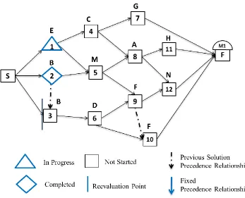
To illustrate the problem under consideration, a sample project network is shown in

Figure 4.1 where an activity on node (AON) representation is utilized. The network is defined by

the set of activities {1, 2, …, 12} and the set of resources {A, B, …, O}. Multiple resource

alternatives with stochastic times and fixed rate costs are available for 8 out of the 12 project

activities. In this sample network, the costs of the activities are dependent on the activity’s

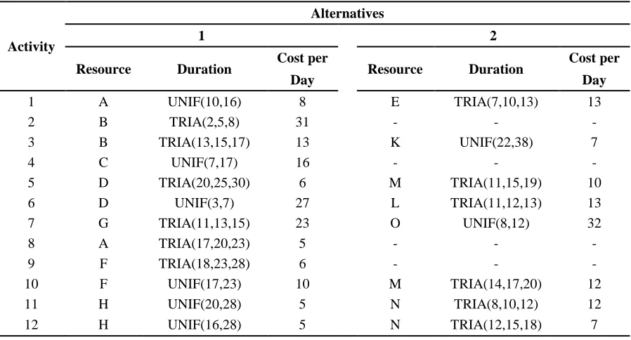
duration, hence, daily costs are provided. Table 4.1 presents the alternatives available for the

project activities. For example, activity one has two potential resource alternatives {A, E}, but

activity two has only one potential resource alternative B. In addition, depending upon the

resource configuration evaluated, precedence decisions may emerge between activities sharing

resources. Table 4.2 shows the activities with potential resource conflict such as {2, 3} which

26

late, a penalty is assessed which is dependent upon the amount of time by which the project is

late.

Figure 4.1 TCRCM Project Network Example – Activities with Multiple Resource Alternatives and Potential Resource Precedence Relationships

Table 4.1 TCRCM – Resource Alternative Stochastic Times and Costs

Activity

Alternatives

1 2

Resource Duration Cost per Resource Duration Cost per

Day Day

1 A UNIF(10,16) 8 E TRIA(7,10,13) 13

2 B TRIA(2,5,8) 31 - - -

3 B TRIA(13,15,17) 13 K UNIF(22,38) 7

4 C UNIF(7,17) 16 - - -

5 D TRIA(20,25,30) 6 M TRIA(11,15,19) 10

6 D UNIF(3,7) 27 L TRIA(11,12,13) 13

7 G TRIA(11,13,15) 23 O UNIF(8,12) 32

8 A TRIA(17,20,23) 5 - - -

9 F TRIA(18,23,28) 6 - - -

10 F UNIF(17,23) 10 M TRIA(14,17,20) 12

11 H UNIF(20,28) 5 N TRIA(8,10,12) 12

27

Table 4.2 TCRCM – Potential Resource Precedence Decisions

Activity Pair

Potential Shared Resource

2,3 B

5,6 D

5,10 M

9,10 F

11,12 H or N

In the sample project network, the target completion time for the project is time 72, and

the equation for the penalty costs associated with late project completion is:

𝑃𝐹(𝑇, 𝜏) = {0, 𝑖𝑓 𝜏 ≤ 72 50(𝜏 − 72), 𝑖𝑓 𝜏 > 72

Ultimately, our objective is to obtain the optimal allocation of resources and resource

precedence relationships that minimize the expected total project cost, where the total cost is

defined as activity costs plus penalty due to project lateness.

The Total Cost Resource Constrained Method (TCRCM) is implemented in two phases.

Prior to the start of the project, the method is used to determine the optimal resource

configuration considering the uncertainty that characterizes a project at the beginning stage. This

is identified as Phase I. The dynamic phase (Phase II), which is implemented as the project

unfolds, considers actual costs and durations of completed and in progress activities to reevaluate

the rest of the project. Hence, during Phase II, only the uncertainty associated with the remaining

activities is considered to identify the optimal resource configuration from that point forward.

The next section describes the general simulation-based optimization approach used by

28

4.1

Overview of the Simulation-Based Optimization Approach

The structure of the simulation-based optimization approach, which is the same for both

Phase I and Phase II, is described in this section. The components that make up the structure of

the method include the input parameters, simulation model, optimization model and output

parameters. During Phase I, uncertainty for all project activities is considered to evaluate the

optimal resource configuration while, in Phase II, actual values are used for completed or in

progress activities and the optimization is done considering the uncertainty of the remaining

activities in the project.

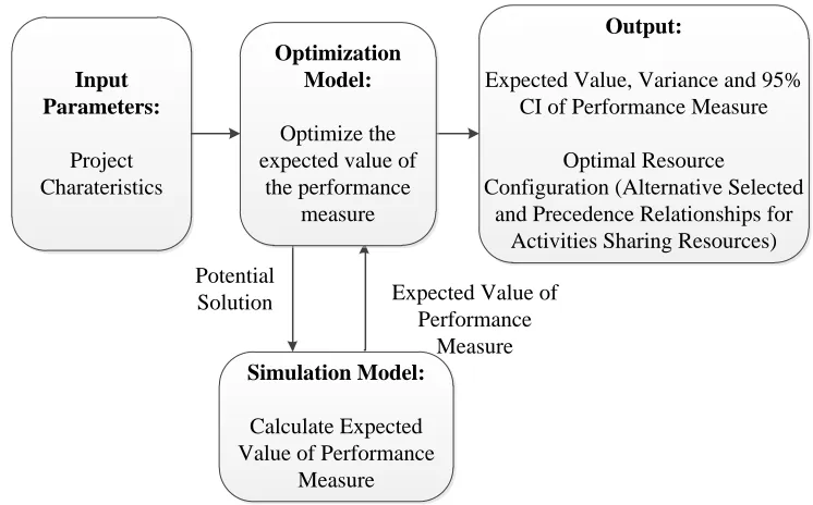
Figure 4.2 illustrates how all the components of the method are linked together. The input

parameters that represent the characteristics of the project network under evaluation are used by

the optimization model to identify potential solutions subject to a set of constraints. The

optimization model determines the values of the decision variables that satisfy the constraints.

Once a feasible solution is identified based on the solution space, the potential solution is sent to

the simulation model in order to simulate instances of the project network and calculate the

expected value of a performance measure (e.g. total project cost). As soon as the simulation

model finishes, the value of the performance measure for the evaluated resource configuration is

returned to the optimization model. This cycle between the optimization model and the

simulation model continues with the purpose of comparing the outcome of different resource

configurations. After the optimal solution has been found, output information regarding the

optimal resource configuration and/or precedence relationships, as well as the value of the

29 Input

Parameters:

Project Charateristics

Output:

Expected Value, Variance and 95% CI of Performance Measure

Optimal Resource

Configuration (Alternative Selected and Precedence Relationships for

Activities Sharing Resources)

Potential

Solution Expected Value of Performance

Measure

Simulation Model:

Calculate Expected Value of Performance

Measure

Optimization Model:

Optimize the expected value of

the performance measure

Figure 4.2 Structure of the Simulation-based Optimization Approach

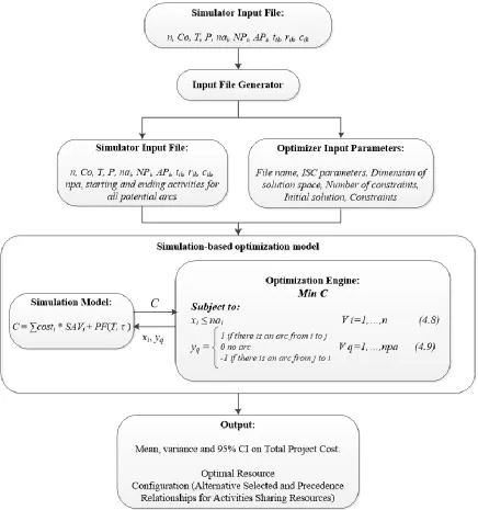
With the optimal solution identified by the optimization model, a project simulator is

used to run multiple replications of the base configuration and the optimal configuration for

comparison purposes. The project simulator components are: the input file, simulation model,

and output file. The input file containing the characteristics of the project and configuration

under evaluation feeds the simulation model. The simulation model runs multiple replications of

the project and provides statistics for project completion time and project cost as an output file.

The following sections describe the general assumptions and modeling details of the

simulation-based optimization approach.

4.1.1 Assumptions

The general assumptions considered in the optimization method include:

 Activity time and cost distributions for all alternative resources can be estimated.

 Activity times are independent.

 Precedence relationships due to technical constraints are defined before the project starts

30

 Penalty costs, represented by a linear function, are defined before the project starts.

 Activities cannot be split or changed once they have begun. That is, once activities have

been started, they will be worked on continuously until finished.

 A single resource/resource set is needed to execute an activity.

 The remaining time and cost for in progress activities can be accurately estimated.

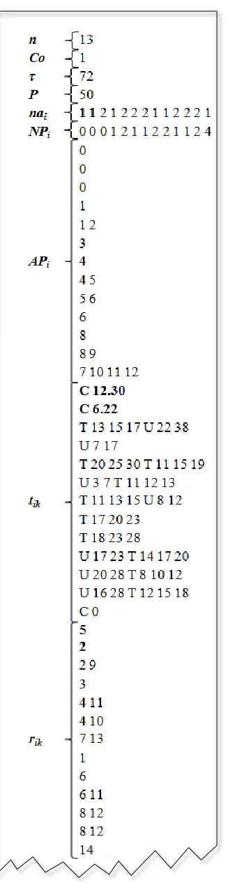
4.1.2 TCRCM: Input Parameters

The input parameters provide information regarding the characteristics of the project

network into the optimization model. The parameters that serve as input to the

simulation/optimization model are the following:

n = number of activities in the project.

Co = time and cost correlation. If Co is equal to 1, time and cost are correlated, 0 otherwise.



P = penalty cost per time unit of tardiness.

i

na = number of resource alternatives of activity i1,...,n.

i

NP = number of predecessors of activity i1,...,n.

i

AP= predecessors of activity i1,...,n.

ik

t = stochastic duration of activity i1,...,n by alternative k 1,...,na.

ik

r = resource of activity i1,...,n by alternative k 1,...,na.

ik

c = stochastic cost (if Co = 0) or daily cost (if Co = 1) of activity i1,...,n by alternative

. ..., ,

1 na

31

4.1.3 TCRCM: Optimization Model

The optimization model receives the input parameters and identifies potential feasible

solutions. Different resource configurations, represented by the values of the decision variables,

are identified. The optimization model interacts with the simulation model to evaluate these

configurations in order to determine the optimal expected total project cost (C) which includes

the activity costs and the penalty costs due to tardiness at project completion.

In order to generate the constraints of the optimization model, the following parameters

are calculated:

PCM= predecessor chain matrix that indicates the complete predecessor chain of activity

n

i1,..., . If PCMij is equal to 1, activity j is included in the predecessor chain of

activityi, 0 otherwise, such that,

             nn n n PCM PCM PCM PCM PCM PCM PCM ... ... ... ... ... ... ... ... ... ... 1 21 1 12 11 .

AM= resource alternative matrix that indicates if resource l 1,...,nr is a potential alternative for activityi1,...,n. If AM_il is equal to 1, resource l can be assigned to activityi, 0 otherwise, such that,

             nnr n nr AM AM AM AM AM AM AM ... ... ... ... ... ... ... ... ... ... 1 21 1 12 11 .

CM= cost matrix that indicates the cost, CMil, of assigning resource l1,...,nr to activity

n

32              nnr n nr CM CM CM CM CM CM CM ... ... ... ... ... ... ... ... ... ... 1 21 1 12 11 .

The values of the following decision variables will be determined by the optimization

model and returned to the simulation model to perform the expected total project cost

calculation:

RM= resource matrix that indicates if activity i1,...,n will be executed by resource l. If

il

RM is equal to 1, resource l is assigned to activityi, 0 otherwise, such that,

             nnr n nr RM RM RM RM RM RM RM ... ... ... ... ... ... ... ... ... ... 1 21 1 12 11 . ij

a = represents the direction of the resource precedence arc between activities and is equal to

1 if an arc is drawn from activityi1,...,n to activity j 1,...,n, 0 otherwise.

ijl

S= indicator variable that equals 1 if the same resource l 1,...,nris assigned to activity i

and activity j, 0 otherwise.

ijl

S= indicator variable that equals 1 if neither activities i or activity j are assigned resource

nr

33 The optimization model is described as follows:

Minimize: _

      



(1 )(1 ) , ,

nr

ij ji ijl ij ji

l

a a S PCM PCM i j i j



 

 _{ }    





1 , , ,

ijl ijl il jl

SS RM RM  i j l i j (4.3)

1 , , ,

ijl ijl

SS  i j l i j (4.4)

l RM

i

il  



l i AM

RM_il  _il  , (4.6)





ij jy yi

a a   a  narcs  (4.7)

The objective function (4.1) minimizes the expected total project cost calculated by the

simulation model. The total project cost includes both, the cost associated with executing the

activities, and the penalty costs due to late project completion. Constraints (4.2), (4.3), and (4.4)

ensure that the resource precedence is only determined between activities that share resources

but do not have a technical precedence. Constraint (4.2) checks if two activities have a technical

precedence, and constraint (4.2) evaluates if the activities share a resource. Constraint (4.4) ties

constraints (4.2) and (4.3) together so that if there are no resources in common, the technical

precedence is not evaluated for those two activities and no arc is drawn between them. In order

to better explain how these constraints work together, let us consider the following: if two

activities have a resource in common, RM_il and RMjl both take on a value of one and, hence,

34

of one which allows constraint (4.2) to evaluate if there is a technical precedence between the

activities. If the activities do not have a technical relationship, PCM_ji and PCM_ij take on a

value of zero and an arc between the activities needs to be drawn. The constraints tie together the

same way for the cases when there are no common resources but there is a technical precedence.

These constraints reduce the number of arcs to be evaluated by restricting the optimization model

to making the resource precedence decisions between activities with potential conflicts.

Constraint (4.5) guarantees that only one resource or resource set is assigned to each

activity of the project. Constraint (4.6) ensures that the resources assigned to a task are only

those eligible resources from among the set of alternatives available for the activity.

The last constraint (4.7) ensures that there are no looping conflicts (tours) when testing

resource precedence relationships during the optimization of a project. In this formula, narcs

represents the number of arcs involved in the looping conflict. A looping conflict can emerge in

cases where three or more activities have a potential resource in common. To illustrate this,

consider the example in Figure 4.3 where three activities {1,2,3} are assigned the same resource,

X. In the absence of any technical precedence arcs, there are three resource precedence decisions

required. The model formulation would result in two constraints of the form of (4.7), such as:

12 23 31 2

a a  a 

13 32 21 2 .

a a  a 

These constraints will prevent a potential tour which would result in an infeasible solution.

35

4.1.4 TCRCM: Simulation Model

Once the optimization model determines a potential solution, this solution is sent to the

simulation model to run multiple project instances of the selected resource configuration. The

decision variables that are manipulated by the optimization model include the resource matrix (

il

RM ) with the resource selected for each activity and the direction of the precedence arc for

those activities that share resources (a_ij). The values of a_ijare directly used in the simulation

model while the resource matrix is translated to the vector, SAV , for convenience in coding.

SAV = selected alternative vector where SAVi indicates the alternative k{1,...,na} _{selected by}

the optimization model for each activity i1,...,n.

In order to construct the SAV vector, the resource matrix (RM_il) is compared to the

resource alternatives matrixr_ik. The model loops through RM_il to determine which resource l is

assigned to each activity i and, comparing this information withrik, the selected alternative for each project activity is identified.

Once the simulation model translates the decision variables obtained from the

optimization model, the simulation model runs in order to calculate the total project cost of the

selected project configuration. The following parameters are created by the simulation model to

simulate the execution of the project. These are constructed either from the values of the

optimization decision variables or the values of the provided input parameters as follows:

i

rnp = number of resource predecessors of activityi1,..,n where rnp_in_j1aij i.

ij

PM = predecessor matrix of technical predecessors that indicates if activity i1,...,n is a

predecessor of activity j1,...,n. If PM_ij is equal to 1, activity i is a predecessor of

36              nn n n PM PM PM PM PM PM PM ... ... ... ... ... ... ... ... ... ... 1 21 1 12 11

The following variables are used as the simulation model runs to identify if an activity is

ready to start. These are compared to rnp_i and NPi in order to determine if all resource and

technical predecessors of an activity are completed.

i

rpc = number of resource predecessors of activity ialready completed i1,...,n

i

PC = number of technical predecessors of activity i already completed i1,...,n

As activities start and finish execution, the following variables are updated to capture the

start and finish times of the activities as well as indicate that they have been completed.

i

st = start time of activity i i1,...,n

i

ct = completion time of activity i i1,...,n

i

CA = is 1 if activity i is completed, 0 otherwise i1,...,n

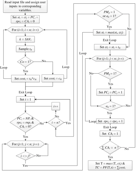
In order to better illustrate how the simulation model works, and how every variable and

calculated parameter binds together, the flow chart shown in Figure 4.4 was provided. First, the

model reads the input file that provides information regarding the characteristics of the project.

Each of the values of the input parameters supplied is assigned to the corresponding variable in

the simulation model. Afterwards, the variables used by the simulation model to check on the

status of activities and the variables used to store start and completion times are set to zero as

their initial state. The