Energy efficient ship operation through speed optimisation in various weather conditions

1

Energy Efficient Ship Operation through Speed

Optimisation in Various Weather Conditions

Tong Cui, Benjamin Howett, Mingyu Kim, Ruihua Lu, Yigit Kemal Demirel, Osman Turan, Sandy Day and Atilla Incecik

Department of Naval Architecture, Ocean and M arine Engineering, University of Strathclyde,

100 M ontrose Street, Glasgow G4 0LZ, UK, tong.cui@strath.ac.uk

Abstract

Speed optimisation or speed management has been an attractive topic in the shipping industry for a long time. Traditional methods just rely on master’s ex-perience. Some recent methods are more efficient but always have many con-straints, which cannot get optimum speed profile. This paper introduces a rela-tively advanced model for speed global optimisation towards energy efficient shipping in various weather conditions and shows the effect when the method is employed. With this model, if a ship type, departure and destination ports and fixed ETA (Estimated Time Arrival) are given, the stakeholders can be provid-ed with a more reasonable speprovid-ed operation plan for a certain commercial route, which leads to lower fuel consumption. Weather conditions and hence routing plays a very important role in this process. Several case studies over different shipping conditions are considered to validate the model.

Keywords

Speed optimisation · Weather routing · Energy efficiency

1

Introduction

Shipping plays an important role in the global economy, as almost 90% goods traded world wide are transported by sea. The Greenhouse Gas (GHG) emissions and the energy consumption from shipping field are significant, wh ich have become very important factors that can not be ignored for both environment and economic b enefit (IMO 2014; IHS Global Insight 2009; Oxford Economics 2014). The modern ship-ping industry is paying more and more attention to energy saving and emission reduc-tion. In recent years, as the main regulatory body for shipping, the International Mar i-time Organisation (IMO) has raised several technical and operational measures t o-wards regulating shipping energy efficiency and thereby controlling the marine GHG emissions. One of the most important concepts is Ship Energy Efficiency Manag e-ment Plan (SEEMP).

The IMO introduced the SEEM P as a mandatory tool under MARPOL Annex VI1 _and

entered into force on January 1, 2013.

There are many categories of energy imp rovement methods for potential adoption within each ship’s SEEMP, including Fuel-efficient Sh ip Operations, Optimised Ship Handling, Hull Maintenance, Propulsion System, Waste Heat Recovery etc. For the category of Fuel-efficient ship operations recommended by SEEM P (IMO 2012), it includes:

- Improved voyage planning - Weather routing

- Just in time - Speed optimisation - Optimized shaft power

Among them, speed optimisation and weather routing are two very co mmon and ef-fective approaches for energy efficient ship operations (IMO 2012, 2016; Simonsen et al 2015).

Speed optimisation means to select an optimu m speed changing strategy for a g iven route, which can make a great contribution to energy efficient shipping. There are many types of research in this field. Several studies assumed the ship speed is fixed (Wang et al 2011, 2012), while several studies also make a speed up or reduction with a certain speed step to see the benefits (Norstad et al 2011; Lu et al 2014). Several studies carried out the speed optimisation based on Historical data and Sea current forecasts (Jussi 2012). Heuristic methods, like genetic, is also used for speed optimisation by Golias et al. (2010), but the optimality cannot be guaranteed. Besides, several studies created the relationship model between fuel consumption and sailing speed (Lang and Veenstra 2010; Du et al. 2011) or even between o il price and sailing speed (D Ronen 2011) for energy efficient s hipping. All of these studies provide very positive methods but still cannot avoid having more or fewer constraints, especially not able to provide accurate ship operations with various weather conditions.

Actually, weather condition is a very important factor, wh ich can not be ignored dur-ing speed optimisation. When combined with weather routdur-ing technique, the speed optimisation will become more reliable. Sh ip weather routing is used to determine the optimu m route (course and speed) between given departure and destination ports based on weather conditions and ship’s corresponding performance. It always aims to minimu m fuel consumption, suitable ETA (estimated time arrival) or maximu m ship safety etc. It has been proven as a very effective tool in shipping field (Simonsen 2015; Chen 1998; Buhaug 2009).

In this paper, a speed optimisation model is developed for energy efficient shipping. This model is composed of several sub-modules, including ship performance

1

3 tion module, grids system design module, weather routing module, etc. Every module has its own task, and every one of them should link with each other so that the whole model can run well towards energy efficient shipping. With the weather routing mo d-ule integrated, this model can predict ship operations in various sea states well. Be-sides, it can also combine with any other technologies very well, like wind assistant, fouling influence prediction etc. Therefore, with so many factors into consideration, this model will certainly provide stakeholders more reliable ship operations for a shipping task.

2

Speed Optimisation Model

The Speed Optimisation Model presented in this paper is not only for single fixed route optimisation but also for global optimisation which also takes the direction optimisation into consideration. According to the requirement fro m stakeholders, the only input items are the ship model, departure time and ETA, positions of departure and destination, and then the model will determine an optimu m route towards min i-mum fuel consumption after complicated calculation.

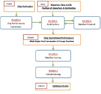
The workflow of the model is shown in Fig.1. It can be seen the model generally co n-tains five modules, and each of them will be introduced briefly as below:

2.1 Module 1: Ship Performance Calculation

Since the speed optimisation model runs towards minimu m fuel consumption under various weather conditions, the ship performance prediction becomes a very important module of the whole model, which should predict ship brake power under different situations very accurately. In this module, the ship particulars including ship geome-try, main engine and propeller parameters should be collected firstly. Next, the ship resistance in calm water can be p redicted based on Holtrop 84 method (Ho ltrop 1984) while the added resistance due to waves and wind can be calculated based on the Kwon’s method (Kwon 2008) a fter weather forecast module is introduced. Based on the total resistance, together with ship speed, propeller open water performance and efficiency of transmission of power, the ship engine brake power can be determined , which is necessary for fuel consumption calcu lation. Besides, the sea trial data, ship model test data or even noon report data can be introduced to verify the predicted ship performance. Based above, when weather data is given, the ship performance in this sea state can be obtained in this module, which will be us ed in weather routing mod-ule afterward.

In order to obtain ship performance very quickly and conveniently, once ship partic u-lars are decided, a ship performance database can be generated before running the whole speed optimisation model. With the g iven variab le (sailing speed, weather data etc), the ship performance can be easily determined through the database. One simple database contains these dimensions: speed, significant wave height, relative wave angle, true wind speed, relative wind angle and an output attribute: brake power (Ho-wett 2015). The ship performance database may also include additional dimensions (eg draft/loading condition) or additional attributes (eg fuel consumption) where re-quired. Therefore, when alternative energy saving techniques or other influencing factors are taken into account, the model only needs to generate a new ship perfo r-mance database without changing anything else. This makes the speed optimisation model combine with other external techniques well.

2.2 Module 2: Grids system

5 five waypoints in next stage. For some special shipping tasks, such as the ship going to several fixed ports during the whole navigation, the grids system can be automati-cally divided into several stages based on the same p rinciple. Besides, for most real situations, the ship always travels around some islands or avoid the prohibited military zone, an area avoidance function is also developed.

Fig. 2A Typical Grids system

It is worth noting that the speed optimisation for a single fixed route (without direc-tion optimisadirec-tion) can be regarded as a special but much easier situadirec-tion within the normal global optimisation. For a fixed route, it must be formed by several certain waypoints as well. The latitude and longitude of every certain waypoint will be input to grids system manually. So that the grids system also has several stages but has only one waypoint, thus, one direction on each stage. The whole speed optimisation will carry out with this simple grids system.

2.3 Module 3: Weather Forecast

This system will take only winds, waves into account at the mo ment. Waves and winds data are both downloaded fro m ECMWF (European Centre fo r Med iu m-Range Weather Forecasts) website. The data is constructed in gridded binary (GRIB) data form, including 10 meter U wind co mponent, 10 meter V wind co mponent, mean wave direction, mean wave period and significant height of co mb ined wind waves and swell, and they all update every 6 hours. These weather data will be converted to Beaufort Nu mber and relative weather direction according to ship heading for ship performance calculation. The weather forecast files are linked with three co mmon parameters: time, latitude and longitude. With given time, latitude and longitude, the weather forecast module will provide corresponding sea conditions to grids system.

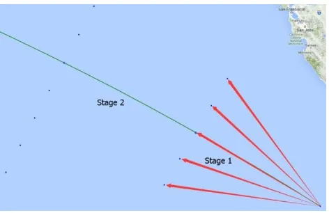
2.4 Module 4: Weather Routing

Fig. 3Ship routing stages

As mentioned in Module 2, the ship will travel from the departure to destination stage by stage (Fig. 3). For the ship in any waypoint, the system reads the weather data at that point in accordance with local longitude, latitude and departure time firstly. Next, a random speed is assigned to a travel direction. This speed ranges from minimum speed to maximu m speed with an interval speed. Having the weather data and ship speed, according to ship performance calculation result, the fuel consumption on this arc is calculated under this speed and direction. Then the navigation information of this arc (fuel consumption, ship speed, navigation duration, local time and coordinates of local departure point) is stored in its arrival point. After that, the ship will travel to next waypoint based on all information saved in this arrival point.

The whole calculation starts from the departure port. Under this simulation principal as described above, the fuel consumption modeling will be continuously utilised for all stages between departure port and destination. This process covers all the speed and direction options. In the end, the total fuel consumption and voyage duration of the different potential route with different speed set will be stored in the destination node. The recorded information will be used to select the minimum fuel consumption route at given ETA, which is regarded as the global optimisation. During the

optimisation process, several smart algorithms are added to the weather routing mo d-ule, which can reduce much calculation time and make the whole calculation run t o-wards the required ETA faster.

2.5 Module 5: Post-processing

7

3

Case studies

A Bulk Carrier with 35,500DWT and 175.72 meters in length is taken as the ship model in the case studies. The shipping area is fro m Dubai to the middle o f the Ind ian Ocean, but the ship should travel along the west end of India. The departure and des-tination points are given as 25°15'N\ 56°51'E and 8°13'S \ 92°22'E respectively. The grids system has 19 stages, and every stage has maximu m 15 vertical waypoints with equal distance of 30 nautical miles. Sh ip speed ranges from minimu m 9 knots to ma x-imum 19 knots with the interval speed 0.1 knot. The required ETA is set at 242 hours.

3.1

Case Study 1

In order to see the benefits of the model, the speed sets under six different conditions are selected for comparison, which are shown as below:

Speed Set A – Actual route and actual voyage speed as recorded in ship noon report Speed Set B – Actual route and optimum speed with identical ETA

Speed Set C – Global Optimisation with identical ETA Speed Set D – Global Optimisation with 3% less ETA Speed Set E – Global Optimisation with 3% more ETA Speed Set F – Global Optimisation with 5% more ETA

Global optimisation means optimise both speed and direction at the same time. So the resulting route may be different fro m the actual route recorded in ship noon report. All of above have same departure time at 2015-05-13, 23:00. The results are shown in Table 1.

As can be seen from Tab le 1, co mpared to Speed Set A, the speed optimisation (Speed Set B) for a fixed route will provide 1.47% fuel savings, while global optimisation (Speed Set C, both speed and direction optimisation) can provide 1.60% fuel savings. For Speed Set D, because it has 3% shorter ETA, the average sailing speed will in-crease, so it will consume 4.43% more fuels. As to Speed Set E with 3% longer ETA and Speed Set F with 5% longer ETA, based on the same reason, they will respectiv e-ly provide 7.05% and 10.2% fuel savings.

Table 1. Comparison of ship operational performance of different speed sets for case study 1 Stage Speed Set A (knots) Speed Set B (knots) Speed Set C (knots) Speed Set D (knots) Speed Set E (knots) Speed Set F (knots)

1 12.5 12.8 13.0 13.0 13.2 12.8

2 12.5 13.2 13.2 13.2 12.6 13.2

3 12.7 12.6 13.0 13.0 12.6 12.6

4 12.5 12.6 13.0 12.6 9.7 12.6

5 12.4 10.7 10.1 11.9 12.6 9.7

6 13.0 12.8 12.6 12.8 11.9 12.6

7 12.8 12.1 12.1 12.1 12.1 11.9

8 12.6 12.6 12.6 13.0 12.6 11.9

9 12.4 13.6 12.6 13.0 12.1 12.6

10 12.1 13.0 12.1 13.0 11.9 11.9

11 13.2 12.6 13.4 13.4 12.6 11.9

12 12.5 13.0 12.6 13.2 12.1 12.6

13 12.4 9.7 12.1 12.6 9.7 9.7

14 12.3 12.1 11.3 12.1 11.9 9.7

15 13.1 12.1 12.1 12.2 12.6 11.9

16 12.9 12.6 12.6 12.6 13.2 12.6

17 12.4 12.8 13.2 13.2 13.4 13.2

18 11.9 13.2 13.0 13.2 13.2 13.2

19 11.8 12.8 13.2 13.4 13.2 13.2

Voyage Duration

(hours)

242 242 242 235 249 254

Fuel Consumption

(tonnes)

135.23 133.24 133.06 141.23 125.69 121.37 Fuel Savings

compared to Speed

9

Fig. 4The speed and weather condition distribution of Speed Set C

Fig.5Optimal routes based on different conditions for case study 1

3.2

Case Study 2

In order to see the speed optimisation benefits under various weather condition more clearly, another three case studies departure at different seasons are carried out. To-gether with the Speed Set C, they are list as below:

Above simu lations have different departure seasons at February, May, August and November, but have same ETA of 242 hours. The results are shown in Table 2.

Table 2. Comparison of ship operational performance of different speed sets for case study 2

Stage

Speed Set G Feb (knots)

Speed Set C May (knots)

Speed Set H Aug (knots)

Speed Set I Nov (knots)

1 13.2 13.0 13.2 12.6

2 13.0 13.2 13.2 11.9

3 11.9 13.0 12.6 11.9

4 11.9 13.0 13.2 11.9

5 11.9 10.1 12.1 13.2

6 11.9 12.6 12.1 11.9

7 11.9 12.1 12.6 11.9

8 12.6 12.6 12.4 11.9

9 11.9 12.6 12.6 11.9

10 13.2 12.1 12.6 11.9

11 13.2 13.4 12.6 13.2

12 13.2 12.6 12.6 13.2

13 12.6 12.1 12.1 13.4

14 9.7 11.3 12.1 12.6

15 12.6 12.1 13.2 13.2

16 13.2 12.6 12.6 12.6

17 13.4 13.2 12.2 12.6

18 13.2 13.0 10.9 12.6

19 13.2 13.2 12.2 12.6

Average BN 3 3.21 3.32 3.05

Voyage

Dura-tion(hours) 242 242 242 242

Fuel Consumption

(tonnes) 132.33 133.06 136.13 135.40

Fuel compared to

Speed Set C (%) 0.54 0 -2.31 -1.76

11 into consideration, it can be found that Speed Set I has relatively mo re head sea and bow sea situations, which will definitely add fuel consumption. Therefore, the results are reasonable.

Fig. 6Speed distribution based on different conditions for case study 2

Fig. 7BN distribution based on different conditions for case study 2

presented speed optimisation model works very well. Besides, all of these routes are drawn on the map in Fig. 9.

Fig. 9Optimal routes based on different conditions for case study 2

4

Conclusion

This paper presents a speed optimisation model towards energy efficient shipping. With the integration of weather routing module, this model can provide stakeholders optimu m ship operations in various weather conditions towards minimu m fuel con-sumption according to the shipping schedule. Several case studies with Bulk Carrier were carried out. As can be seen from results, this model can help the case study ship-ping save almost 1.5% fuel consumptions, which proves the model works well.

Of course, during the speed optimisation process, there are always many uncertainties like the quality of ship performance prediction, weather forecasting limitations, ser-vice speed estimations or even operating profile o f the engine etc, which always make the final result not reliable enough. In the future, the detailed research will be contin-ued to improve this speed optimisation model further.

13

Acknowledgements

This research is part of the project: Sh ipping in Changing Climates (EPSRC Grant no. EP/K039253/1). The author would like to express sincere thanks for the support from UK Research Council, University of Strathclyde and China Scholarship Council.

Reference

Buhaug Ø, Corbett JJ et a l (2009). Prevention of air pollution fro m ships – second IMO GHG study, International Maritime Organization, London, UK.

Chen H, Ca rdone V and Lacey P (1998) Use of operation support informat ion tec h-nology to increase ship safety and efficiency, SNAME transactions, 106, 105-127

Du Y, Chen Q, Quan X er al (2011) Be rth allocation considering fuel consumption and vessel emissions. Transportation Research 47E, 1021–1037

Go lias M.M, Bo ile M, Theofanis S, Efstathiou C (2010) The berth scheduling pro b-le m: ma ximizing berth productivity and min imizing fuel consumption and e missions production. Transportation Research Record 2166, 20–27

HOLTROP J (1984) A Stat istical Re -Analysis of Resistance and Propulsion Data. International Shipbuilding Progress, 31(363), 272-276

HOW ETT B (2015) Report: SHIP PERFORMANCE PROFILE FILE FORMAT DEFINITION

IHS GLOBA L INSIGHT (2009) Va luation of the liner shipping industry -Economic contribution and liner industry operations

IMO (2012) Guidelines for the development of a SEEMP. MEPC 63/23, Annex 9

IMO (2014) Third IMO GHG Study 2014 – Exceutive Summary and Final Report

IMO (2016) Guidelines for the development of a SEEMP. MEPC 70/18/Add.1, Annex 10

Jussi P (2012) Overco ming the challenges in vessel speed optimization, HANSA In-ternational Maritime Journal, 149. Jahrgang – 2012 – Nr.9, 130-135

Kwon Y.J. (2008) Speed Loss Due To Added Resistance in Wind and Waves. The Naval Architect, Vol. 3, 14-16

Lu R, Cui T, Turan O, Boulougouris E (2015) Speed manage ment for energy effic ient shipping, 2015 SCC Conference, UK

Norstad I, Fagerholt K, Laporte G (2011) Tra mp ship routing and scheduling with speed optimization. Transportation Research Part C: Eme rging Technologies, 19, 853-865

Oxford Economics (2014) The economic value of the EU shipping industry

Ronen D (2011) The effect of oil price on containership speed and fleet size. Journal of the Operational Research Society 62, 211–216

Simonsen MH, Larsson E, Mao W, Jonas W R (2015). State-of-the-art within ship weather routing. Proceedings of the ASME 34th International Conference on Ocean, Offshore and Arctic Engineering, St. John's, Newfoundland, Canada, OMAE

Wang S, Meng Q (2011) Schedule design and container routing in liner shipping. Transportation Research Record 2222, 25–33.

Wang S, Meng Q (2012) Liner ship fleet deployment with container transshipment operations, Transportation Research Part E 48, 470–484