City, University of London Institutional Repository
Citation
:
Asimit, A.V. ORCID: 0000-0002-7706-0066, Gao, T., Hu, J. and Kim, E. (2018).
Optimal Risk Transfer: A Numerical Optimisation Approach. North American Actuarial
Journal, 22(3), pp. 341-364. doi: 10.1080/10920277.2017.1421472
This is the accepted version of the paper.
This version of the publication may differ from the final published
version.
Permanent repository link: http://openaccess.city.ac.uk/id/eprint/21931/
Link to published version
:
http://dx.doi.org/10.1080/10920277.2017.1421472
Copyright and reuse:
City Research Online aims to make research
outputs of City, University of London available to a wider audience.
Copyright and Moral Rights remain with the author(s) and/or copyright
holders. URLs from City Research Online may be freely distributed and
linked to.
City Research Online:
http://openaccess.city.ac.uk/
[email protected]
Alexandru V. Asimit1
Cass Business School, City, University of London, London EC1Y 8TZ, United Kingdom. E-mail: [email protected]
Tao Gao
Department of Mathematical Sciences, University of Bath, Bath BA2 7AY, United Kingdom.
E-mail: [email protected]
Junlei Hu
Cass Business School, City, University of London, London EC1Y 8TZ, United Kingdom. E-mail: [email protected]
Eun-Seok Kim
School of Business and Management, Queen Mary, University of London, London E1 4NS, United Kingdom. E-mail: [email protected]
December 15, 2017
Abstract: Capital efficiency and asset/liability management are part of the Enterprise
Risk Management Process of any insurance/reinsurance conglomerate and serve as
quan-titative methods to fulfill the strategic planning within an insurance organisation. There
has been a considerable amount of work in this ample research field, but invariably one of
the last questions is whether or not, numerically, the method is practically implementable,
which is our main interest. The numerical issues are dependent upon the traits of the
optimisation problem and therefore, we plan to focus on the optimal reinsurance design,
which has been a very dynamic topic in the last decade. The existing literature is
fo-cused on finding closed-form solutions that are usually possible when economic, solvency,
etc constraints are not included in the model. Including these constraints, the optimal
contract can only be found numerically. The efficiency of these methods is extremely
good for some well-behaved convex problems, such as the Second-Order Conic Problems.
Specific numerical solutions are provided in order to better explain the advantages of
ap-propriate numerical optimisation methods chosen to solve various risk transfer problems.
The stability issues are also investigated together with a case study performed for an
insurance group that aims capital efficiency across the entire organisation.
Keywords and phrases: Linear Programming, Optimal Reinsurance/Risk Transfer, Risk Measure, Second-Order Conic Programming.
1. Introduction
Various actuarial problems involve decision-making procedures that evaluate the most favourable risk
position of an insurance company. For example, capital efficiency and asset/liability management are
part of the Enterprise Risk Management Process of any insurance/reinsurance conglomerate and serve
as quantitative methods to fulfill the strategic planning within the organisation. The decision-makers are
prone to combine expert judgment with core quantitative methods, which involve numerical optimisation
and often, intensive computing skills. Therefore, many optimisation problems are not practically
imple-mentable in a straightforward manner to practitioners and academics that are not operation research
inclined. Unfortunately, numerical issues are anecdotally disregarded and for this reason, we aim to
implement optimisation algorithms that are hardly accessible to non-specialists in this field. In order to
better communicate the advantages and caveats of possible solutions, we plan to focus on optimal risk
transfer problems, but the numerical methods are transferrable skills when implementing other actuarial
problems.
Consider a two-player insurance setting where the first player is the risk holder who transfers a portion
of its risk to the second player. At the same time, the second player charges the first player to cover its cost
of transfer. This setting includes a very common risk transfer, known asreinsurance, where the two players are known as the insurer and the reinsurer respectively; the transfer cost is known as the reinsurance premium. The primary aim of optimal reinsurance design is to find the ‘best’ trade-off between risk-bearing and profit-earning. The Stop-Loss reinsurance contract is optimal when minimising the variance
of an insurer’s retained risk is considered (see Borch, 1960) or when maximising the expected utility of
insurer’s final wealth (see Arrow, 1963). After the two pioneering works, optimal reinsurance problems
have been widely studied in various settings. For example, Gajek and Zagrodny (2000) and Kaluszka (2001
and 2004) have studied the variance-minimisation problem with premium principles including standard
deviation premium principle and mean-variance premium principle. In recent years, the risk-measure
based optimal reinsurance model has received vast attention. Two commonly used risk measures, Value-at-risk(VaR) andConditional Value-at-risk(CVaR), are treated by Cai and Tan (2007), Caiet al.(2008), Cheung (2010), Asimit et al. (2013c) and Cui et al. (2013). On the other hand, optimal reinsurance problems modeled with multiple risks or counterparty default risks are investigated by Bernard and
Ludkovski (2012), Cai and Wei (2012), Asimitet al.(2013a) and Caiet al.(2014).
As anticipated, a risk transfer is not always made in between two players, which is possible if multiple
reinsurance players accept to share the risk with one insurer or a pool of insurers. Alternatively, one
can place this risk sharing problem in the context of an insurance group that intends to achieve capital
efficiency (see Asimit et al., 2013b and Asimit et al., 2016). This standard risk management tool aims to reduce the capital requirements for an insurance group that has multiple legal entities with specific
regulatory requirements, where many economic constraints are usually imposed internally and externally.
The problem is not tractable in closed-form solutions due its complexity, and therefore, it is rarely
discussed in the literature.
So far, the omnipresent model risk, i.e. the risk of choosing a wrong model, has been fashionably
same problem arises if data do not reflect the future predictions, especially in extreme scenarios where
expert opinion is the usual choice for practitioners. In any of these cases, the underlying model is not
unknowable, but unknown, and the decision-maker is exposed to a higher level of uncertainty when robust
decisions are sought. Robust optimisation is precisely the standard method that helps in reducing the
model risk and it has been translated in the optimal reinsurance context by Balb´as et al. (2015) and Asimit et al. (2016). At a superficial level, one may think that the risk level increases as a result of conservative/robust decisions, which in fact is not true, since the main aim is to reduce the change in
the chosen decision, if the “true” model would have been known. Thus, this na¨ıve perception is actually
not true for robust optimised decisions and it would be interesting to show how one can take advantage
of computational methods when searching for robust decisions, rather than focusing on model-specific
closed-form solutions.
We have tried to justify, by discussing various strands of research on optimal risk transfers, but beyond
the optimal reinsurance problem, why numerical methods are of interest. Our goal is now to demonstrate
that computations are possible in an efficient manner. In the context of optimal reinsurance design,
the efficiency of the numerical methods is high for some particular convex problems as justified in Tan
and Weng (2014). This excellent paper provides the way forward in solving optimisation problems of
that type when multiple business lines and/or other risks (such as background, counterparty default and
model risks) are included in the model.
The remainder of this paper is organised as follows. Section 2 introduces the background knowledge of
this paper including some key definitions. Formulations of intended optimisation problems are explained
in Section 3. The uncertainty of model choice is discussed by analysing worst-case models in Section 4.
Section 5 provides numerical examples, while the main conclusions of the paper are summarised in
Section 6. All proofs are relegated in Section 7.
2. Background
Consider a two-player (only for simplicity, but further generalisations are possible) insurance setting
where the first player holds m lines of business (LOB) with random risks, denoted as X1, . . . , Xm,
which is defined on a probability space (Ω,E,P) with Ω ⊆ <+. Assume that for each of the risksXk,
k∈ M:={1, . . . , m}, the first insurance player transfersI2k[Xk] to a secondary player, and its remaining
risk becomesI1k[Xk] =Xk−I2k[Xk]. There also exists a cost of transfer denoted byP. Consequently,
the after-transfer risk positions of the two players becomes
m
X
k=1
I1k[Xk] +P and m
X
k=1
I2k[Xk]−P.
The risk preferences of the first and second player are represented by arisk measure (RM) denoted as ρ1 and ρ2, respectively. Thus, there is a rationality constraint that both players’ after-transfer risk
position should be no worse than their before-transfer position. That is,
ρ1
m
X
k=1
I1k[Xk] +P
!
≤ρ1
m
X
k=1 Xk
!
and ρ2
m
X
k=1
I2k[Xk]−P
!
≤ρ2(0). (2.1)
Definition 2.1. Let(Ω,E,P)andX be a probability space and a linear space of random variables onΩ, respectively. A RMρ:X → < is translation invariant if
ρ(X+a) =ρ(X) +a for anyX ∈ X anda∈ <.
The comonotonic property of ρ requires that ρ X+f(X)
= ρ(X) +ρ f(X)
for any X ∈ X and non-decreasing function f.
Ifρ1andρ2 have thetranslation invariant property, the rationality constraints in (2.1) become
max
( P , ρ2
m
X
k=1 I2k[Xk]
!)
≤P ≤min
( P , ρ1
m
X
k=1 Xk
!
−ρ1
m
X
k=1 I1k[Xk]
!)
, (2.2)
whereP is the minimum charge that the second player will agree in a transfer, whileP is the maximum price that the first player is prepared to pay in exchange for a risk transfer.
The set of possible ceding functions must satisfyI1k ∈ I:={f : 0≤f(x)≤x}, for all 1≤k≤mand
the set of feasible contracts, A consists of elements (I11, . . . , I1m, P)∈ Im× <. Alternatively, in order
to avoid potential moral hazard issues, the set of feasible contracts can be defined byAco consisting of
elements (I11, . . . , I1m, P)∈ Icom× <, where ceding functions are comonotone
Ico :={f : 0≤f(x)≤x, f(x) andx−f(x) are non-decreasing inx∀x}.
The risk transfer cost P is based on the second player’s risk preference and is usually based on another
RM, Π(·) such that
m
X
k=1
Π I2k[Xk]
≤P. Without loss of generality, it is assumed that the second player
has the same preference for all LOBs, but otherwise, the numerical technologies can be easily adapted.
There is a vast literature on RMs and it would be impossible to discuss all of them in one paper, but
we will focus on the most sensible ones that are socially accepted among academics and practitioners:
the classical standard deviation, the class of coherent RMs discussed in the seminal paper of Artzner
et al.(1999) and the well-known VaR. All of these RMs are formally defined now.
Definition 2.2. Let b ∈ <+ andZ be a random risk defined on (Ω,E,P). The standard deviation RM
is given byρ(Z) =EZ+bSd(Z), whereSd(·)is the usual standard deviation.
A RM islaw-invariantif the risk measurement is solely based on the risk distribution, i.e. risks equally distributed are measured with the same exposure and all RMs are assumed to satisfy this property. One
of the most used RMs in practice that is not coherent is VaR. By definition, the VaR of a generic loss
variableZ at a confidence levela, VaRa(Z), is thea%-quantile, i.e.
VaRa(Z) := inf{z≥z0: Pr(Z≤z)≥a},
where z0 := sup{z ∈ <: Pr(Z ≤z) = 0} represents the left-end point of the distribution function ofZ. By convention, inf∅:= +∞and sup∅:=−∞. The class of coherent RMs consists of law-invariant RMs
that aremonotone, translation invariant, positive homogeneous and sub-additive (for details, see Artzner
et al., 1999). The subclass of coherent RMs that possesses the comonotonic property is known as the
Definition 2.3. Let g: [0,1]←[0,1]be a distortion function, i.e. non-decreasing and concave function such that g(0) = 0 and g(1) = 1. Denote φ(·) := g0(1− ·). Then a distortion RM has the following representationρg(Z) :=
R1
0 φ(a)VaRa(Z)da, where the random riskZ is on(Ω,E,P).
Note that the derivative ofgis understood as the right derivative, whenever it does exist, which may not exist for at most a countable set, due to the concavity property ofg. A well-known distortion RM is CVaR with distortion functiong(x) = x
1−a∧1, wherex∧z:= min(x, z). CVaR has appeared in various
forms in the literature (see Acerbi and Tasche, 2002), but we prefer using the following representation
CVaRa(Z) := inf t∈<
t+ 1
1−aE(Z−t)+
, where (x)+:= max(x,0), (2.3)
as first defined in Rockafeller and Uryasev (2000), due to its computational advance.
Not all coherent RMs are comonotonic, and a large parametric subclass of coherent RMs that are not
comonotonic is introduced by Fischer (2003) as follows:
Ψα(Z) :=EZ+λ
E(Z−EZ)α+ 1/α
with 0≤λ≤1, 1≤α≤ ∞,
whereα=∞in the above is read asEZ+λV aR1(Z)−E(Z).
3. Empirical Risk Transfer Models
This section first describes the main optimal risk transfer problem to be solved by using our numerical
methods. We further explain the one LOB case and extend these results for the multiple LOBs by
providing formulations that can be implemented and solved in an efficient manner.
3.1. Main optimisation problem. The main problem that we propose to investigate is the weighted
average of two insurance players under various economic and/or rationality constraints like (2.2); its
mathematical formulation is as follows:
min
(I11,...,I1m)∈ AorAco;P∈<
( δ1ρ1
m
X
k=1
I1k[Xk]+P
!
+δ2ρ2
m
X
k=1
Xk−I1k[Xk]−P
!)
s.t.
m
X
k=1
Π Xk−I1k[Xk]
≤P, P ≤P ≤P , (3.1)
ρ1
m
X
k=1
I1k[Xk]
!
+P≤ρ1
m
X
k=1 Xk
! , ρ2
m
X
k=1
Xk−I1k[Xk]
!
≤P.
where δ1, δ2 ≥0. The above contains the risk sharing problems, where the players cooperate to reduce their risks, known as Pareto efficient transfers, and under certain conditions, the set of these transfers are as given in the above-mentioned problem (see, for example, Aase 2002). The risk sharing problem
may require to optimise overAco if the moral hazard is highly likely. Risk transfers within an insurance
group do not involve moral hazard, since each legal entity is owned in a certain proportion by the
same owner, and therefore, the feasibility set is A. Setting, (δ1, δ2) equal to (1,0) or (0,1), then (3.1) becomes a standard optimal reinsurance contract evaluated from the point of view of the first and second
insurance player, respectively. We believe that formulation (3.1) is a fairly general problem and it worth
The optimisation problem (3.1) has infinite dimension, as one needs to search over all possible ceding
functions of I1k, k ∈ M. This issue can be overcome by reformulating (3.1) into a discretised setting.
Assume that a sample of sizen, denoted by xk = (xk1, . . . , xkn)T, is available forXk, k∈ M. This is
possible if historical data is available, otherwise, a socially accepted proxy model can be used to draw
those samples. For each observed lossxki,i= 1, . . . , n, we assume that the first player transferszkiand
retainsyki:=xki−zki. Consequently, the decision variables,I1k, I2k,k∈ M, in (3.1) can be replaced by
vectors yk = (yk1, . . . , ykn)T and zk = (zk1, . . . , zkn)T respectively, and hence, the infinite-dimensional
optimisation problem (3.1) can be translated into the following (n×2m+ 1)-dimensional problem. Now, if we optimise over A, the risk transfers should satisfy yk ≤xk,zk ≤xk andyk+zk =xk for
allk∈ M. Recall that the inequality (equality) between two vectors is understood componentwise, i.e.
a≤b(a=b) if and only ifai≤bi (ai=bi) for alli. For a givenk∈ M, an allocation yk,zk
ofxk is
feasible inAco if the vectors are increasingly ordered. That is,
0≤yki≤xki,0≤yk,i+1−yki, ∀i= 1,2, . . . , n,
0≤zki≤xki,0≤zk,i+1−zki, ∀i= 1,2, . . . , n,
yki+zki=xki, ∀i= 1,2, . . . , n,
or equivalently,
0≤yki≤xki, yk,i+1−yki≤xk,i+1−xki, ∀i= 1,2, . . . , n,
0≤zki≤xki, zk,i+1−zki≤xk,i+1−xki, ∀i= 1,2, . . . , n,
yki+zki=xki, ∀i= 1,2, . . . , n.
The latter could be written as follows:
Ayk≤Axk,Azk ≤Axk,yk+zk =xk,
where then×nmatrixAis defined by
A:=
1 0 · · · 0
−1 1 · · · 0 . .. . ..
0 0 · · · 1
.
Various problems that we further investigate are convex and reducible toSecond Order Conic Program-ming (SOCP). SOCP problems are convex optimization problems in which a linear function is minimised over the intersection of various second-order (quadratic) cones. The standard form of SOCP has the
following representation
min x
aT1x s.t. kBlx+blk ≤cTlx+dl, l= 1, . . . , L, Bx=a2,
wherea1∈Rn, Bl∈Rnl×n, bl∈Rnl, c
l∈Rn, dl∈R, B∈Rp×n, a2∈Rp. In addition,k·krepresents
theEuclidean distance, i.e. kxk :=
n
X
i=1 x2i
!1/2
. A more concise introduction and summary on SOCP
can be found in the Appendix of Tan and Weng (2014).
SOCP problems have received considerable attention from researchers due to its wide range of
methods that have been developed for such optimisation problems. The study of primal-dual interior
point methods for SOCP problems started with Nesterov and Todd (1997, 1998). These authors presented
their results in the context of optimisation over self-scaled cones, which includes the class of second-order
cones as a special case. Their work culminated in the development of a particular primal-dual method
called the NT method. Adler and Alizadeh (1995) studied the relationship between semi-definite
prob-lems, SOCP and the specialised so-calledXZ+ZX method of Alizadeh et al. (1998) to SOCP. Then, Alizadeh and Schmieta (1997) gave non-degeneracy conditions for SOCP and developed a numerically
stable implementation of theXZ+ZX method; this implementation is used in the SDPpack software package. Subsequently, Monteiro and Tsuchiya (2000) proved that this method, and hence, all members
of the Monteiro-Zhang family of methods, have a polynomial iteration complexity. The computational
ef-fort of solving SOCP with a standard form isO L1/2
iterations ofO n2Pn
l
in the case of primal-dual
interior-point method. In practice, the special structure (e.g., sparsity) often allows solving the SOCP
more efficiently. There are now several packages available that may handle SOCP problems such as the
SDPpack package noted above and the Sturm’s SeDuMi, which is another widely available package that
is based on the Nesterov-Todd method.
Because of SOCP’s broad applicability and computational tractability, there are many studies showing
classes of optimisation problems that could be reformulated as SOCP problems. Although it may be
possible to formulate an optimisation problem as an SOCP, the task may be far from being trivial. For
example, problems withhyperbolic constraintsare SOCP representable by using the fact that a constraint of the form
wTw≤xy, wherew∈ <n, x, y∈ <+,
is equivalent to the following second-order cone constraint
2w
x−y
≤ x+y.
For further details about transforming many kinds of constraints into second-order cone inequalities, we
refer the reader to Loboet al. (1998) and Alizadeh and Goldfarb (2003).
The RMs in (3.1) are replaced by their sample estimators. LetZ be a discrete random variable with possible outcomes{z1, . . . , zn}, each having the same chance to occur. Thus, the standard deviation RM
from Definition 2.2 is replaced by its unbiased estimator, n11Tz+b√kQzk
n−1, where the n×n matrixQis
defined as
Q:=
1−1
n −
1
n · · · −
1
n
−1
n 1−
1
n · · · −
1
n
..
. ... . .. ...
−1
n −
1
n · · · 1−
1
n
.
By definition, 0and 1are column vectors of zeros and ones, respectively, where the dimension is not
explicitly given. The unbiased estimator is advisable for relatively large values of n, while the biased estimator (with√n−1 replaced by√n) is more appropriate for smalln.
The VaR and all other distortion RMs dependent on the ordering ofzi’s. Letz(1) ≤z(2)≤. . .≤z(n)
function. Now, distortion RMs are a tad more cumbersome and its computational complexity largely
depends on whether or not the sample is ordered. That is, if the sample is increasingly ordered,z(i)=zi
for all 1≤i≤n, then
ρg(Z) = n
X
i=1
g (n−i+ 1)/n
−g (n−i)/n
zi. (3.2)
Otherwise,
ρg(Z) = n
X
i=1
g (n−i+ 1)/n−g (n−i)/nz(i)
=
n
X
i=1
g (n−i+ 1)/n
−g (n−i)/n
(n−i+ 1)CVaR(i−1)/n(Z)−(n−i)CVaRi/n(Z)
= b01Tz+
n−1 X
i=1
biCVaRi/n(Z),
whereb0= 1−g (n−1)/nandbi= (n−i)
2g (n−i)/n−g (n−i+ 1)/n−g (n−i−1)/nfor all 1≤i≤n−1.
3.2. One LOB case. It is first assumed that m = 1 in order to elaborate the simplest (3.1)-type
optimisation problems that one may have. Recall that ordered samples simplify the estimators that are
based on VaR or any other distortion RM.
Problem 3.1. Assume that (3.1)is optimised over Aco and without loss of generality x1 is assumed to
be increasingly ordered. Moreover, ρ1(·) = VaRa(·), ρ2(·) =E(·) +bSd(·)and Π(·) =ρg(·). Therefore,
the following optimisation problem needs to be solved:
min
(y1,z1,P)∈ <n×<n×<
(δ1−δ2)P+δ1y1a∗+δ2
1
n1
Tz
1+b
kQz1k
√
n−1
s.t. 1
n1
Tz
1+b
kQz1k
√
n−1 ≤P, P ≤P≤P , (3.3)
y1a∗+P ≤x1a∗, aTz1≤P,
Ay1≤Ax1,Az1≤Ax1,y1+z1=x1,
wherea∗=dnaeis a scalar andai=g (n−i+1)/n
−g (n−i)/n
for all1≤i≤ndue to equation(3.2).
It is not difficult to show that Problem 3.1 is in fact of the SOCP-type. One may show (as explained
in the beginning of the proof of Theorem 3.1) that (3.3) is solved by
min
(y1,z1,P,t)∈ <n×<n×<×<
(δ1−δ2)P+δ1y1a∗+δ2 1
n1
Tz
1+ bt
√
n−1
s.t. 1
n1
Tz
1+ bt
√
n−1 ≤P, P ≤P ≤P ,
y1a∗+P ≤x1a∗, aTz1≤P, kQz1k ≤t,
Ay1≤Ax1,Az1≤Ax1,y1+z1=x1.
Problem 3.1 can be easily adapted whenρ1is a distortion RM, since y1is increasingly ordered and thus,
Problem 3.2. Assume that (3.1)is optimised overAand without loss of generalityx1 is assumed to be
increasingly ordered. Moreover, ρ1(·) = CVaRa(·), ρ2(·) = E(·) +b Sd(·) and Π(·) =ρg(·). Therefore,
the following optimisation problem needs to be solved:
min
(y1,z1,P)∈ <n×<n×<
(δ1−δ2)P+δ1min
s1∈<
s1+ 1
n(1−a)1
T(y
1−s11)+ +δ2 1 n1 Tz
1+b
kQz1k
√
n−1
(3.4)
s.t. 1
n1
Tz
1+b
kQz1k
√
n−1 ≤P, P ≤P ≤P ,
min
s1∈<
s1+ 1
n(1−a)1
T(y
1−s11)+
+P ≤CVaRa(X1),
b01Tz1+
n−1 X
i=1 bimin
ci∈<
ci+
1
n−i1
T(z
1−ci1)+
≤P,
y1≤x1,z1≤x1,y1+z1=x1,
whereCVaRa(X1)is a scalar and it can be found via (3.2).
Theorem 3.1 shows that Problem 3.2 can be reduced to an SOCP representation and its proof is
relegated to Section 7.
Theorem 3.1. If δ1> δ2>0, then Problem 3.2 is solved by the following SOCP:
min
(y1,z1,u1,w,P,s1,r1,t,e,c)∈<n×<n×<n
×<n×(n−1)×<×<×<×<×<n−1×<n−1
(δ1−δ2)P+δ1r1+δ2 1 n1 Tz 1+ bt √
n−1
s.t. 1 n1 Tz 1+ bt √
n−1 ≤P, P ≤P ≤P , kQz1k ≤t, (3.5)
s1+ 1
n(1−a)1
Tu
1≤r1, 0≤u1, y1−s11≤u1,
r1+P ≤CVaRa(X1), b01Tz1+
n−1 X
i=1
biei≤P,
ci+
1
n−i1
Tw
i≤ei, 0≤wi, z1−ci1≤wi, ∀i= 1, . . . , n−1,
y1≤x1,z1≤x1,y1+z1=x1.
The case in which 0< δ1=δ2 is not covered by Theorem 3.1 and a different reformulation is needed. It is not difficult to find that the optimisation problem (3.4) becomes in this setting as follows:
min
(y1,z1)∈<n×<n
min
s1∈<
s1+ 1
n(1−a)1
T(y
1−s11)+
+
1
n1
Tz
1+b
kQz1k
√
n−1
(3.6)
s.t. max
( P ,1
n1
Tz
1+b
kQz1k
√
n−1, b01
Tz
1+
n−1 X
i=1 bimin
ci∈<
ci+
1
n−i1
T(z
1−ci1)+ )
≤min
P ,CVaRa(X1)−min s1∈<
s1+ 1
n(1−a)1
T(y
1−s11)+
,
while the optimalP is any value that satisfies the first constraint. Then, (3.6) is solved by the following SOCP:
min
(y1,z1,u1,w,s1,r1,t,e,c)∈<n×<n×<n
×<n×(n−1)×<×<×<×<n−1×<n−1
r1+
1
n1
Tz
1+ bt
√
n−1
s.t. s1+ 1
n(1−a)1
Tu
1≤r1, 0≤u1, y1−s11≤u1,kQz1k ≤t, (3.7)
s1+
1
n(1−a)1
Tu
1≤CVaRa(X1)−P ,
s1+
1
n(1−a)1
Tu
1+
1
n1
Tz
1+ bt
√
n−1 ≤CVaRa(X1),
s1+ 1
n(1−a)1
Tu
1+b01Tz1+
n−1 X
i=1
biei≤CVaRa(X1),
1
n1
Tz
1+ bt
√
n−1 ≤P , b01
Tz
1+
n−1 X
i=1
biei≤P ,
ci+
1
n−i1
Tw
i≤ei, 0≤wi, z1−ci1≤wi, ∀i= 1, . . . , n−1,
y1≤x1,z1≤x1,y1+z1=x1.
The latter equivalence could be proved in a similar manner as Theorem 3.1 is justified and therefore, its
proof is left to the reader.
Unfortunately, the 0< δ1< δ2 case makes the Problem 3.2 not tractable. The lack of convexity leads
only to reformulations that are not computationally efficient and for this reason, we do not further discuss
such a setting. In fact, all the remaining optimisation problems assume thatδ1> δ2 >0, but one could
follow the same reasons as used in the reformulation (3.7), whenever the 0< δ1=δ2 setting is in place. It would be interesting to point out that solving Problem 3.2 over Aco is a tad simpler. Thus, if x1
andy1 are increasingly ordered, then Problem 3.2 is simplified to solving:
min
(y1,z1,P)∈ <n×<n×<
(
(δ1−δ2)P+ δ1
n(1−a) (a
∗−na)y1 a∗+
n
X
i=a∗+1 y1i
!
+δ2 1
n1
Tz
1+b
kQz1k
√
n−1
)
s.t. 1
n1
Tz
1+b
kQz1k
√
n−1 ≤P, P ≤P ≤P , 1
n(1−a) (a
∗−na)y
1a∗+
n
X
i=a∗+1 y1i
!
+P ≤CVaRa(X1),
b01Tz1+
n−1 X
i=1 bimin
ci∈<
ci+
1
n−i1
T(z
1−ci1)+
≤P,
As before, the above is solved by the following SOCP:
min
(y1,z1,w,P,t,e,c)∈<n×<n
×<n×(n−1)×<×<×<n−1×<n−1
(
(δ1−δ2)P+ δ1 n(1−a) (a
∗−na)y
1a∗+
n
X
i=a∗+1 y1i
!
+δ2 1 n1 Tz 1+ bt √
n−1
) s.t. 1 n1 Tz 1+ bt √
n−1 ≤P, P ≤P ≤P , kQz1k ≤t, b01
Tz
1+
n−1 X
i=1
biei≤P,
1
n(1−a) (a
∗−na)y1 a∗+
n
X
i=a∗+1 y1i
!
+P≤CVaRa(X1),
ci+
1
n−i1
Tw
i≤ei, 0≤wi, z1−ci1≤wi, ∀i= 1, . . . , n−1,
0≤Ay1, y1≤x1, y1+z1=x1,
where the proof is once again left to the reader, since it requires similar arguments as we have seen before.
Problem 3.3. Assume that (3.1)is optimised overAand the moral hazard is only removed for the first
player. Thus, without loss of generality x1 and y1 are assumed to be increasingly ordered. Moreover, ρ1(·) = VaRa(·),ρ2(·) =E(·) +b Sd(·) andΠ(·) =ρg(·). Therefore, the following optimisation problem
needs to be solved:
min
(y1,z1,P)∈ <n×<n×<
(δ1−δ2)P+δ1y1a∗+δ2
1
n1
Tz
1+b
kQz1k
√
n−1
s.t. 1
n1
Tz
1+b
kQz1k
√
n−1 ≤P, P ≤P ≤P , y1a∗+P≤x1a∗,
b01Tz1+
n−1 X
i=1 bimin
ci∈<
ci+
1
n−i1
T(z
1−ci1)+
≤P,
0≤Ay1, y1≤x1, y1+z1=x1,
which can be solved efficiently as shown in Theorem 3.2.
Theorem 3.2. If δ1> δ2>0, then Problem 3.3 is solved by an SOCP given by:
min
(y1,z1,w,P,t,e,c)∈<n×<n
×<n×(n−1)×<×<×<n−1×<n−1
(δ1−δ2)P+δ1y1a∗+δ2 1 n1 Tz 1+ bt √
n−1
s.t. kQz1k ≤t,
1 n1 Tz 1+ bt √
n−1 ≤P, P ≤P ≤P ,
b01Tz1+
n−1 X
i=1
biei≤P, y1a∗+P≤x1a∗,
ci+
1
n−i1
Tw
i ≤ei, 0≤wi, z1−ci1≤wi, ∀i= 1, . . . , n−1,
0≤Ay1, y1≤x1, y1+z1=x1.
The next setting aims to illustrate how to deal with non-comonotone RMs and we choose those defined
by Fischer (2003).
Problem 3.4. Assume that (3.1)is optimised overAand the moral hazard issues are removed from the
ordered. Moreover, ρ1(·) = VaRa(·), ρ2(·) =E(·) +b Sd(·) andΠ(·) = Ψα(·). Therefore, the following
optimisation problem needs to be solved:
min
(y1,z1,P)∈ <n×<n×<
(δ1−δ2)P+δ1y1a∗+δ2 1
n1
T
z1+b
kQz1k
√
n−1
s.t. 1
n1
Tz
1+b
kQz1k
√
n−1 ≤P, P ≤P ≤P , y1a∗+P≤x1a∗,
1
n1
Tz
1+λ
1
n
n
X
i=1
z1i−
1
n1
Tz
1 α
+ !1/α
≤P,
0≤Ay1, y1≤x1, y1+z1=x1.
Problem 3.4 can be efficiently solved ifα∈ {1,2} and the corresponding reformulations are given in Theorem 3.3.
Theorem 3.3. Assume that δ1> δ2>0. Ifα= 1, then Problem 3.4 is solved by the following SOCP:
min
(y1,z1,P,t,u)∈ <n×<n×<×<×<n
(δ1−δ2)P+δ1y1a∗+δ2
1
n1
Tz
1+ bt
√
n−1
s.t. kQz1k ≤t,
1
n1
Tz
1+ bt
√
n−1 ≤P, P ≤P ≤P , 1
n1
Tz
1+ λ n
n
X
i=1
ui≤P, y1a∗+P≤x1a∗,
0≤ui, z1i−
1
n1
Tz
1≤ui, ∀i= 1, . . . , n,
0≤Ay1, y1≤x1, y1+z1=x1.
If α= 2, then Problem 3.4 is solved by an SOCP given by:
min
(y1,z1,P,t,u)∈ <n×<n×<×<×<n
(δ1−δ2)P+δ1y1a∗+δ2 1
n1
Tz
1+ bt
√
n−1
s.t. kQz1k ≤t,
1
n1
Tz
1+ bt
√
n−1 ≤P, P ≤P ≤P , 1
n1
Tz
1+ λ
nkuk ≤P, y1a∗+P≤x1a∗,
0≤u, z1−
1
n1
Tz
11≤u, ∀i= 1, . . . , n,
0≤Ay1, y1≤x1, y1+z1=x1.
3.3. Multiple LOBs case. When the insurance players have more then one LOB, the numerical methods
are similar to what we have seen earlier. For the ease of exposition, assume now that m= 2. Unfortu-nately, even ifxk,yk andzk are increasingly ordered fork= 1,2, none ofx1+x2,y1+y2orz1+z2are
ordered. Therefore, unlike the one LOB case, the empirical representation of V aRwith multiple LOBs cannot be written as a linear function of decision variables even if the optimisation problem is solved
overAco. In fact, if ρ1 or ρ2 is VaR, our model (3.1) becomes a non-convex optimisation problem, and
non-convex component can be written as a difference of two convex functions (including VaR). In
techni-cal terms, iterations between the primal space and the dual space finally lead to a convergence (see Tao
and An, 1998). The DCA has not been used in the actuarial literature, but has been successfully applied
by Wozabal et al.(2010) in the classical portfolio investment optimisation. However, as emphasised in Tao and An (1998), the nature of the optimum obtained from DCA depends on the starting point chosen
by the algorithm, and hence, it is not computationally efficient in solving our optimisation model (3.1)
and we choose not to provide details on them..
Problem 3.5. Assume that ρ1(·) = CVaRa(·), ρ2(·) = E(·) +b Sd(·) and Π(·) = ρg(·). Moreover,
the portfolio consists of two independent LOBs and (3.1) is optimised overA. Therefore, the following optimisation problem needs to be solved:
min
(y1,y2,z1,z2,P)∈ <n×<n×<n×<n×<
(δ1−δ2)P+δ1min
s∈<
s+ 1
n(1−a)1
T(y
1+y2−s1)+
+δ2 1
n1
T(z
1+z2)+b r
kQz1k2+kQz2k2 n−1
!)
s.t. 1
n1
T(z
1+z2)+b r
kQz1k2+kQz2k2
n−1 ≤P, P ≤P ≤P ,
min
s∈<
s+ 1
n(1−a)1
T(y
1+y2−s1)+
+P ≤CVaRa(X1+X2),
b01T(z1+z2) +
n−1 X
i=1 bimin
ci∈<
ci+
1
n−i1
T(z
1+z2−ci1)+
≤P,
yk≤xk,zk≤xk,yk+zk=xk, k∈ {1,2},
whereCVaRa(X1+X2)is a scalar and it can be found via (3.2).
Theorem 3.4. If δ1> δ2>0, then Problem 3.5 is solved by the following SOCP:
min
(y1,y2,z1,z2,u,w,P,s,r,t,e,c)∈<n×<n×<n×<n
×<n×<n×(n−1)×<×<×<×<×<n−1×<n−1
(δ1−δ2)P+δ1r+δ2 1
n1
T(z
1+z2)+ bt
√
n−1
s.t. 1
n1
T(z
1+z2)+ bt
√
n−1≤P, P≤P≤P , k ˆ
Qz12k ≤t,
s+ 1
n(1−a)1
Tu≤r, 0≤u, y
1+y2−s1≤u,
r+P ≤CVaRa(X1+X2), b01T(z1+z2) +
n−1 X
i=1
biei≤P,
ci+
1
n−i1
Tw
i≤ei, 0≤wi, z1+z2−ci1≤wi, i= 1, . . . , n−1,
yk≤xk,zk≤xk,yk+zk=xk, k∈ {1,2},
wherezT
12= (zT1,zT2)andQˆ is an 2n×2nblock matrix given by:
ˆ
Q:=
Q 0 0 Q
As a final note, recall thaty1+y2 is not ordered, even ify1andy2 are increasingly ordered.
Conse-quently, further simplifications to Problem 3.5 (when optimisation is made overAco) are not possible in
the same way that we have found for Problem 3.2.
4. Robust Optimisation
It has been assumed throughout Section 3 thatxk,k∈ M, is drawn from a proxy model. In general,
uncertainty related to the underlying probability measure corresponding to the proxy model exists, and
there may be many possible choices to model the corresponding probabilities. It is assumed in the current
section that the buyer’s and seller’s set of beliefs (about the underlying probability measure) belong to
{P1, . . . ,PN}. That is, the buyer and seller model the uncertainty in a way that their risk measurements
are calculated with respect to some index setsS1,S2⊆ {1, . . . , N}, which is indicated by
ρ1 ·;Pi and ρ2 ·;Pj with i∈ S1, j∈ S2.
Letpikl:=Pi Xk =xkl,xk= xk1, . . . , xkn T
andpik= pik1, . . . , pikn T
. Note thatpik= 1n1, i.e. Pi
is the empirical distribution where each possible outcome{xk1, xk2, . . . , xkn}has the same chance to occur.
That is, the proxy model assumed throughout Section 3 is a potential candidate ofP ∈ {P1,P2, . . . ,PN}.
Models other than the empirical distribution can be obtained by discritising various fitted models. For
example, letFi(·) =Pi(Xk ≤ ·) with k∈ Mdenoting the cumulative distribution function (cdf) of Xk
underPi, then
pikl=Fi
x
k,l+1+xkl
2 ; ˆν
−Fi
x
kl+xk,l−1
2 ; ˆν
for alli= 1,2, . . . , N, k∈ Mandl= 1,2, . . . , n,
where ˆνis the set of parameter estimates obtained via various estimation methods such as the Maximum Likelihood estimation. By convention,xk0=−∞andxk,n+1= +∞. More details about the construction
of candidate models can be found in Asimit et al. (2017). The LOBs are assumed to be independent of each other, which helps us to write the model in a simpler way, but the lack of independence does
not create additional computational effort. Thus, instead of solving the optimisation problem (3.1), the
followingworst-case model is proposed: min
(I11,...I1m)∈ AorAco;P∈<
max
(i,j)∈ S1×S2
( δ1ρ1
m
X
k=1
I1k[Xk]+P;Pi
!
+δ2ρ2
m
X
k=1
Xk−I1k[Xk]
−P;Pj
!)
(4.1)
s.t. max
l∈S2
m
X
k=1
Π Xk−I1k[Xk];Pl≤P, P ≤P ≤P ,
ρ1
m
X
k=1
I1k[Xk];Pi
!
+P≤ρ1
m
X
k=1 Xk
!
, ∀i∈ S1,
ρ2
m
X
k=1
Xk−I1k[Xk]
;Pj
!
≤P, ∀j∈ S2.
More details about the worst-case formulation, its advantages and caveats can be found in Asimitet al.
(2017). Recall that without loss of generality, sample sizes are the same amongst all LOBs, an assumption
that enables reduction in the notation abuse that we inevitably rely on during this paper.
Before giving some examples of (4.1) we need to define the risk measurements under various probability
such thatP(Z=zl) =pl. One may show that the standard deviation underP is
Sd Z;P
=kQz˜ k, where q˜l1l2 =
√
pl1 1{l1=l2}−pl2
for all 1≤l1, l2≤n,
where by definition, 1A represents the indicator operator corresponding to set A that equals to 1 if A
is true and 0 otherwise. Recall that when we work with the empirical measure, i.e. pi = 1/n for all
1 ≤ i ≤ n, then standard deviation has a correction factor ofpn/(n−1) in order to recover the use of the standard sample variance unbiased estimator, which appears in all examples from Section 3. The
correction factor is advisable for reasonable sized samples and not for small samples. The current section
discusses robust formulations and therefore, it is expected to be in a situation where data scarcity is
present; the correction factor does not further appear in the case of empirical probability measure. Thus,
the standard deviation RM ofXk underPi is given by
pTikxk+bkQ˜ikxkk, where q˜l1l2ik=
√
pikl1 1{l1=l2}−pikl2
for all 1≤l1, l2≤n.
The CVaR formulation from (2.3) now becomes
CVaRa Xk;Pi= inf t∈<
t+ 1
1−ap
T
ik xk−t1+
.
Other distortion RMs than CVaR depend on the knowledge of sample ordering. Whenever the sample is
known to be in ascending order, we may write
ρg Xk;Pi
=
n
X
l=1
g 1− l−1 X
s=1 piks
!
−g 1− l
X
s=1 piks
!! xkl.
If there is no piece of information regarding the sample ordering, then distortion risk measures are more
cumbersome and for this reasons, this section avoids dealing with non ordered samples when distortion
risk measures other than CVaR are involved.
4.1. One LOB case. The case in which there is one single LOB, i.e. m= 1, is not difficult and not
very different than the their non-robust counterpart. To make our point, only one example is discussed
in details and is given by Problem 4.1.
Problem 4.1. Assume that (4.1)is optimised over Aco and without loss of generality,x1 is assumed to
be increasingly ordered. Moreover, ρ1(·) =ρg(·),ρ2(·) =E(·) +b Sd(·)and Π(·) = (1 +θ)E(·), θ >0,
implying the following optimisation:
min
(y1,z1,P)∈ <n×<n×<
max
(i,j)∈ S1×S2
n
(δ1−δ2)P+δ1˜aTi1y1+δ2
pTj1z1+bkQ˜j1z1k o
s.t. max
l∈S2
pTl1z1 ≤ P
1 +θ, P ≤P≤P ,
˜
aTi1y1+P ≤a˜Ti1x1, ∀i∈ S1,
pTj1z1+bkQ˜j1z1k ≤P, ∀j∈ S2,
Ay1≤Ax1, Az1≤Ax1, y1+z1=x1,
wherea˜i1:= (ai11, . . . , ai1n)T withai1l=g 1− l−1 X
s=1 piks
!
−g 1− l
X
s=1 piks
!
We are now able to transform the above into an SOCP that can be efficiently solved using standard
commercial solvers.
Theorem 4.1. If δ1> δ2>0, then Problem 4.1 is solved by
min
(y1,z1,P,r,t1 )∈ <n×<n×<×<×<m
r
s.t. (δ1−δ2)P+δ1˜aTi1y1+δ2 pTj1z1+btj1≤r, ∀(i, j)∈ S1×S2,
˜
aTi1y1+P ≤a˜Ti1x1, P ≤P ≤P , kQ˜j1z1k ≤tj1, ∀(i, j)∈ S1× S2,
pTj1z1+btj1≤P, pTj1z1≤ P
1 +θ, ∀j∈ S2,
Ay1≤Ax1, Az1≤Ax1, y1+z1=x1,
wherem=|S2| is the cardinality ofS2.
4.2. Multiple LOBs case. Robust optimisation with multiple LOBs is a difficult problem when dealing
with distortion RMs since the ordering is not preserved when summing the risks. The mathematical
for-mulation of the latter statement is that X1+Y1, X+Y
may not be a comonotone vector even if X1, X
and Y1, Y
are comonotone vectors. Reformulations are possible, though a tad more cumbersome than
what we have seen by now, if CVaR is not used to order the buyer and/or seller risk preferences. Once
again, for the ease of exposition, it is assumed an insurance portfolio consisting of two LOBs, i.e. m= 2.
Problem 4.2. Assume that ρ1(·) = CVaRa(·), ρ2(·) = E(·) +b Sd(·) and Π(·) = (1 +θ)E(·), θ >0.
Moreover, the portfolio consists of two independent LOBs and (4.1) is optimised over A. Thus, the following optimisation problem must be solved:
min
(y1,y2,z1,z2,P)∈ <n×<n×<n×<n×<
max
(i1,i2,j1,j2 )∈ S1×S1×S2×S2
(δ1−δ2)P+δ1min
s∈<
s+ 1
1−aq
T
i1i2(y1+y2−s1)+
+δ2
pTj
11z1+p
T j22z2+b
q
kQ˜j
11z1k
2+kQ˜
j22z2k
2
s.t. max
(l1,l2 )∈
S2×S2
pTl
11z1+p
T l22z2 ≤
P
1 +θ, P ≤P≤P ,
min
s∈<
s+ 1
1−aq
T
i1i2(y1+y2−s1)+
+P≤CVaRa X1+X2;Qi1i2
, ∀ i1, i2∈ S1×S1,
pTj11z1+pTj22z2+b
q
kQ˜j11z1k2+kQ˜j22z2k
2≤P, ∀ j1, j2
∈ S2× S2,
yk ≤xk, zk ≤xk, yk+zk=xk, k∈ {1,2},
where the probability measureQi1i2 assigns the mass as follows
qi1i2 := (qi1i21, . . . , qi1i2n)
T with q
Theorem 4.2. If δ1> δ2>0, then Problem 4.2 is solved by the following SOCP:
min
(y1,y2,z1,z2,w,s,e,P,r,t)∈<n×<n×<n×<n
×<n×m2×<m2×<m2×<×<×< r
s.t.(δ1−δ2)P+δ1ei1i2+δ2 p
T j11z1+p
T j22z2+bt
≤r, ∀(i1, i2, j1, j2)∈ S1×S1×S2×S2,
P ≤P ≤P , pTl
11z1+p
T l22z2≤
P
1 +θ, ∀(l1, l2)∈ S2×S2,
ei1i2+P≤CV aRa(X1+X2;Qi1i2), si1i2+
1 1−aq
T
i1i2wi1i2≤ei1i2, ∀(i1, i2)∈ S1×S1,
0≤wi1i2,y1+y2−si1i21≤wi1i2, ∀(i1, i2)∈ S1×S1,
pTj11z1+pjT22z2+bt≤P, k
ˆ
Qj1j2z12k ≤t, ∀(j1, j2)∈ S2× S2,
yk ≤xk, zk ≤xk, yk+zk =xk, k∈ {1,2},
wherem=|S1| andQˆj1j2 is an 2n×2nblock matrix given by:
ˆ
Qj1j2:=
˜
Qj11 0
0 Q˜j22
.
5. Numerical Illustrations
The current section is dedicated to providing numerical illustrations related to our previous
optimi-sation problems and not only. We first discuss the stability and consistency of the numerical results in
Subsection 5.1, while Subsection 5.2 focuses on a case study about capital efficiency within an IG.
5.1. Stability and consistency. The main aim is to provide analyses on the stability and consistency
of the empirical results for Problem 3.1. We adopt a procedure which is similar to the one presented
in Tan and Weng (2014). Recall that when we solve the empirical optimisation model (3.3), M={1}
and for each given samplex1 = x11, . . . , x1n T
, we find the optimal solutionsy∗1= y∗11, . . . , y∗1nT
and
z∗1 = z11∗ , . . . , z1∗nT
. The solutions are called stable if we expect that the optimal solutions y∗1 and z∗1
always have the same functional form for a given x1. Consistency occurs when we expect that y∗1 and
z∗1converge as the sample sizenincreases. Sincey1∗+z∗1=x1, it is only sufficient to study stability and
consistency forz∗
1. All optimisations are implemented on a desktop with 4 core Intel i7-3770 at 3.40GHz,
16GB RAM, running Linux x64, MATLAB R2014b, CVX 2.1.
The parametrisation for the Problem 3.1 assumes a Pareto lossX1with Pr(X1> x) =x+22,000,000
3
for
all x > 0, δ1 = 0.8, δ2 = 0.2, b = 0.5, P = 0 and P = 5,000. The scatter plots of z∗1 against x1 are
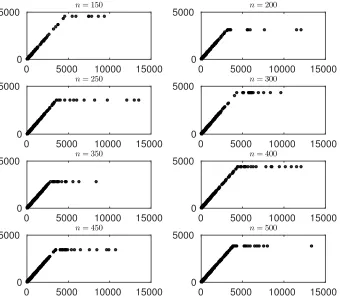
shown in Figure 5.1 for Pareto loss samples and various sample sizesn. Our first observation is that the empirical solutions mimics the functional form of z∗1i =x1i∧d, where d is a constant for i= 1, . . . , n.
Thus, it is useful to fit c(x1i−d1)+∧c(d2−d1) based on our data x1i, z1∗i
for all i = 1, . . . , n and estimate the three parameters using theOrdinary Least Square (OLS) regression. Note that we expect the estimates of ˆc and ˆd1 to be very close to 1 and 0, respectively. Furthermore, the goodness of fit is
tested by introducing an admissibility criterion. That is, the estimated pair of (ˆc,dˆ1,dˆ2) is said to be
admissible whenever
z
∗
1i−ˆc x1i−d1ˆ+∧cˆ d2ˆ −d1ˆ
< ε ∀i= 1, . . . , n,
0 5000 10000 15000 0
5000
n= 150
0 5000 10000 15000
0 5000
n= 200
0 5000 10000 15000
0 5000
n= 250
0 5000 10000 15000
0 5000
n= 300
0 5000 10000 15000
0 5000
n= 350
0 5000 10000 15000
0 5000
n= 400
0 5000 10000 15000
0 5000
n= 450
0 5000 10000 15000
0 5000
[image:19.612.125.465.98.405.2]n= 500
Figure 5.1. Empirical solutions of z∗1 for Problem 3.1 with Pareto loss and various
sample sizesn.
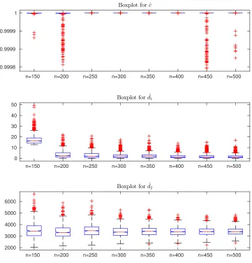
We draw 1,000 random samples fromX1for various sample sizes{150,200,250,300,350,400,450,500}
and estimate the three parameters. Boxplots of those estimates are shown in Figure 5.2. The lower and
upper edge of each box represents respectively the lower and upper quartile, while the short line inside
the box represents the median. The end-point of each whisker represents the minimum or maximum
point estimate that is not an outlier, while outliers are marked as crosses inside the plot. Note that an
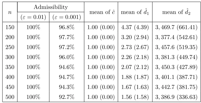
outlier is a point estimate which is away from the box for more than 1.5 times the interquartile range. While Figure 5.2 gives a graphical illustration of (ˆc,dˆ1,dˆ2), Table 5.1 provides a numerical summary.
The evidence provided by Figure 5.2 and Table 5.1 is overwhelming. First of all, we notice that when
ε = 1%, the admissibility is 100% for all sample sizes. If ε is reduced to 0.1%, admissibility is still over 92% for all sample sizes. Recall that we expect the estimates of ˆc and ˆd1 to be close to 1 and 0,
respectively. The slope estimates are perfect, while a small variation from the null value is observed
for d1. Thus, we can conclude that our empirical results are very stable in terms of the shape of the functional form ofz∗i1=xi1∧d. Also, we notice that the standard errors are continuously decreasing as
the sample sizenincreases and therefore, we may conclude the consistency.
n=150 n=200 n=250 n=300 n=350 n=400 n=450 n=500 0.9998
0.9999 0.9999 1
Boxplot for ˆc
n=150 n=200 n=250 n=300 n=350 n=400 n=450 n=500 0
10 20 30 40 50
Boxplot for ˆd1
n=150 n=200 n=250 n=300 n=350 n=400 n=450 n=500 2000
3000 4000 5000 6000
[image:20.612.113.474.101.477.2]Boxplot for ˆd2
Figure 5.2. Boxplots of fitted ˆc, ˆd1and ˆd2 for empirical solutions to Problem 3.1 with
Pareto loss distribution and various sample sizesn.
5.2. Case Study. Consider anInsurance group (IG)with twolegal entities (LE), LE1 and LE2. Their
total future liabilities are denoted as X1 and X2, respectively. With the opportunity of risk sharing amongst the LEs, LE1 transfersI21[X1] to LE2 and retainsI11[X1] =X1−I21[X1], while LE2 transfers
I12[X2] to LE1 and retains I22[X2] = X2−I12[X2]. Also, assume that both LE1 and LE2 are CVaR-regulated, and hence, their risk preferences are given by
ρk(·) :=E(·) +λk CVaRa(·)−E(·)
for k∈ {1,2}.
Recall that the CVaR-based risk capital approach is implemented within the Swiss Solvency Test (the
reg-ulatory environment in Switzerland) and our setting is realistic for such IG. This setting aims to produce
capital efficiency for an IG that operates in various insurance markets that are CVaR-regulated or the
n Admissibility mean of ˆc mean of ˆd1 mean of ˆd2
(ε= 0.01) (ε= 0.001)
[image:21.612.129.465.79.252.2]150 100% 96.8% 1.00 (0.00) 4.37 (4.39) 3,469.7 (661.41) 200 100% 97.7% 1.00 (0.00) 3.20 (2.94) 3,377.4 (542.61) 250 100% 97.2% 1.00 (0.00) 2.73 (2.67) 3,457.6 (519.35) 300 100% 96.0% 1.00 (0.00) 2.26 (2.18) 3,381.3 (449.74) 350 100% 94.6% 1.00 (0.00) 2.07 (2.12) 3,450.3 (427.89) 400 100% 94.7% 1.00 (0.00) 1.88 (1.87) 3,401.1 (387.71) 450 100% 94.3% 1.00 (0.00) 1.67 (1.63) 3,442.7 (381.75) 500 100% 92.7% 1.00 (0.00) 1.56 (1.58) 3,386.9 (336.63)
Table 5.1. Proportion of admissible fitted solutions based on 1,000 samples from a
Pareto loss and various sample sizes n. The last three columns summarise the mean values and standard errors of the estimates.
n 150 200 250 300 350 400 450 500 Time (seconds) 0.90 1.24 2.75 3.33 6.14 7.32 12.59 17.36
Table 5.2. Average run-time for various sample sizesn
For example, Solvency II (the European Union regulatory regime) is a VaR-based environment, but Swiss
Solvency Test and Solvency II are considered equivalent by both parties. An IG has to meet the
regula-tory capital requirements at the IG level (based on the consolidated balance sheet) and at the individual
level. Therefore, we intend to analyse the aggregate capital efficiency by meeting the requirements at
the individual level, which is more stringent due to the IG diversification effect that is in place when risk
capital is set based on the consolidated balance sheet. For mathematical purposes, the confidence levela
could take different values, but due to the equivalence principle, it would be unrealistic to assume such
a scenario. Moreover, the risk preferences from above follow the well-known Cost-of-Capital approach
andλ1, λ2are some parameters (usually greater than 6%) that reflect the cost of using the shareholders’ capital that is very sensitive to the tax regime. The Cost-of-Capital is very sensible to the level of taxation
and therefore, it is realistic to assume thatλ16=λ2. Thus, our risk transfer problem is given by
min
(I11,I12)∈I×I
ρ1 I11[X1] +I12[X2]+ρ2 X1+X2−I11[X1]−I12[X2] , (5.1)
s.t. ρ1 X1−I11[X1]≤C1, ρ2 I12[X2]≤C2,
where C1 and C2 are the asset fungibility limit for LE1 and LE2 respectively. A standard regulatory
constraint is to impose limits for asset transfer, which makes the assets to not be fully fungible, as we
actually assume. Note that the risk transfers are not necessarily comonotone as it is assumed in Asimitet al. (2013b), where a similar, but unconstrained problem, is investigated. The objective function (5.1) can be further written as
E X1+X2
+λ1 CVaRa(T1)−ET1
+λ2 CVaRa(T2)−ET2
[image:21.612.147.452.323.359.2]withT1=I11[X1] +I12[X2] andT2=X1+X2−I11[X1]−I12[X2]. Note thatE(X1+X2) is a constant,
and hence solving (5.1) is equivalent to solve the following infinite dimensional optimisation problem:
min
(I11,I12)∈I×I
λ1 CVaRa(T1)−ET1
+λ2 CVaRa(T2)−ET2 ,
s.t. ρ1 X1−I11[X1]
≤C1, ρ2 I12[X2]
≤C2.
This means that after sampling fromX1 andX2 and using similar notations to those used in Sections 3 and 4, our aim is to solve the following finite dimensional optimisation problem
min
(y1,y2,z1,z2 )∈ <n×<n×<n×<n
λ1min
s1∈<
s1+ 1
n(1−a)1
T(y
1+y2−s11)+
−λ1
n1
T(y
1+y2) (5.2)
+λ2min
s2∈<
s2+
1
n(1−a)1
T(z
1+z2−s21)+
−λ2
n1
T(z
1+z2)
s.t. 1−λ1
n 1
Tz
1+λ1min
s3∈<
s3+ 1
n(1−a)1
T(z
1−s31)+
≤C1
1−λ2 n 1
Ty
2+λ2min
s4∈<
s4+
1
n(1−a)1
T(y
2−s41)+
≤C2,
yk ≤xk, zk ≤xk, yk+zk =xk, k∈ {1,2}.
As it has been done earlier, we further reformulate (5.2) in a way to enable efficient computations.
Theorem 5.1. Problem (5.2)is solved by the next LP:
min
(y1,y2,z1,z2,u1,u2,u3,u4,s,r)∈ <n×<n×<n×<n×<n×<n×<n×<n×<4×<4
M
λ1r1+λ2r2−λ1
n1
T(y
1+y2)− λ2
n1
T(z
1+z2)
+r3+r4
(5.3)
s.t. 1−λ1
n 1
Tz
1+λ1r3≤C1,
1−λ2 n 1
Ty
2+λ2r4≤C2,
s1+
1
n(1−a)1
Tu
1≤r1, 0≤u1, y1+y2−s11≤u1, s2+ 1
n(1−a)1
Tu
2≤r2, 0≤u2, z1+z2−s21≤u2, s3+
1
n(1−a)1
Tu
3≤r3, 0≤u3, z1−s31≤u3, s4+ 1
n(1−a)1
Tu
4≤r4, 0≤u4, y2−s41≤u4,
yk≤xk, zk ≤xk, yk+zk =xk, k∈ {1,2},
whereM is a very large number.
One would wonder how large M should be. If X1 and X2 are non-negative liabilities, as we have assumed by now, then if one aims to solve (5.3) accurate ton1decimal places, then
M >10n1max
C1 λ1
,C2 λ2
would be a good choice. For details, see the proof of Theorem 5.1 that is given in Section 7.
We are now ready to elaborate a numerical illustration for a fictitious IG such the future liabilitiesX1
andX2 are LogNormal distributed and their means and squared coefficients of variation are
Plausible choices for the cost-of-capital rates are λ1 = 10% and λ2 = 12%. The choice of a= 99% is
made as it is the case within the Swiss regulatory environment. We setCk= 40%×ρk Xk
fork∈ {1,2}. Three dependence models for the liabilities are assumed
(A) Independence;
(B) Gaussian copula with parameterρ; (C) Pareto copula.
Recall that the Pareto copula is given by
C(u, v;δ) :=(1−u)−1/δ+ (1−v)−1/δ−1 −δ
+u+v−1, 0≤u, v≤1, δ >0.
(for details, see Nelsen, 2006). The strength of dependence in the upper tail is known as the upper tail dependence coefficient. This measure of dependence equals 2−δ for the Pareto copula and 0 for (A) and
(B). Recall that this measure of dependence is an asymptotic value and one should differentiate between
(A) and (B). When ρ > 0, as we assume a positive dependence among the risks, the Gaussian copula allows a stronger dependence for concomitant extreme events than the independence case, and it is even
stronger asρincreases. The Pareto copula allows a strong dependence, the strongest amongst the three dependence models, which decreases asδincreases.
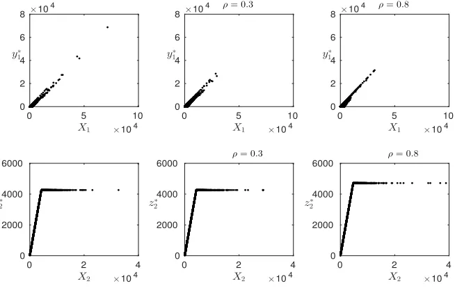
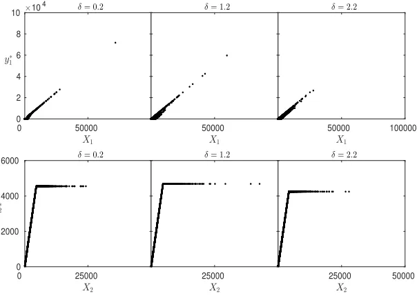
The numerical illustrations are based on a sample size n= 9,000 and we have experienced compu-tational difficulties for samples larger than 10,000, but we believe than a sample of 9,000 is sufficiently informative for our purposes. The optimal solutions ofy∗1 andz∗2 are presented by several scatter plots.
Recall that y∗1 andz∗2 represent the optimal level of risks retained by LE1 and LE2, respectively. The
scatter plots for the three dependence models are displayed in Figures 5.3 and 5.4
X1 ×104
0 5 10
y∗ 1
×104
0 2 4 6 8
X2 ×104
0 2 4
z∗ 2
0 2000 4000 6000
X1 ×104
0 5 10
y∗ 1
×104
0 2 4 6 8
ρ= 0.3
X2 ×104
0 2 4
z∗ 2
0 2000 4000 6000
ρ= 0.3
X1 ×104
0 5 10
y∗ 1
×104
0 2 4 6 8
ρ= 0.8
X2 ×104
0 2 4
z∗ 2
0 2000 4000 6000
[image:23.612.137.464.444.651.2]ρ= 0.8
Figure 5.3. Empirical solutions of y∗1 and z∗2 for Model (A) (left column) and Model
(B) withρ∈ {0.3,0.8} (middle and right column).
Figures 5.3 and 5.4 show thaty∗1mimics a straight line, which suggests that a proportional risk transfer
X1 0 50000 y∗
1 ×104
0 2 4 6 8
10 δ= 0.2
X2 0 25000 z∗
2
0 2000 4000
6000 δ= 0.2
X1 50000
δ= 1.2
X2 25000
δ= 1.2
X1
50000 100000 δ= 2.2
X2
[image:24.612.145.447.88.304.2]25000 50000 δ= 2.2
Figure 5.4. Empirical solutions ofy∗1 andz∗2for Model (C) withδ∈ {0.2,1.2,2.2}.
imposed by LE2. Therefore, two estimations via OLS (as detailed earlier) are further performed:
y1∗i=θ x1i and z1∗i=c min x1i, d
for alli∈ {1, . . . , n}
The results are summarised in Table 5.3.
Parameter Model (A) Model (B) Model (C)
ρ= 0.3 ρ= 0.8 δ= 0.2 δ= 1.2 δ= 2.2
θ 0.6635 0.6551 0.7670 0.8437 0.7734 0.6872
c 1.000 1.000 1.000 1.000 1.000 1.000
d 4,264.8 4,264.2 4,716.4 4,548.0 4,681.9 4,243.7
Table 5.3. Estimates for θ,c anddfor various dependence models.
It becomes clear from Table 5.3 that non-trivial proportional risk sharing is optimal for LE1, while a
stop-loss risk sharing is optimal for LE2. The reason that LE2 prefers to release a high layer is due to a
higher cost of capital faced in its jurisdiction. LE1 and LE2 retain more risk for themselves (estimates
of ˆθ and ˆd are increasing) if stronger dependence in the upper tail is observed. This is not surprising to observe a reduction of the diversification effect as a result of an increased dependence of concomitant
extreme events. The asset fungibility constraints have an important effect over the optimal risk sharing
and the immediate effect is that LE1 prefers a proportional “reinsurance” for its risk, which would not
have happened otherwise. It is well-known that an unconstrained risk sharing problem does not allow
[image:24.612.136.464.457.551.2]6. Conclusions
It is well-known that many actuarial applications involve optimisation and we have tried to provide
some of them related to risk sharing that may arise in many forms. Further, we have shown how one
may reduce those optimisation problems to efficient and reliable computations. These methods may be
extended to many other applications via similar ideas. We have shown that the results are credible by
performing stability and consistency checking. The final numerical example is meant to fully explain how
a practical problem may be implemented via existing optimisation techniques.
7. Proofs
The proof of Theorems 3.2-3.4, 4.1 and 4.2 are very similar to the proof of Theorem 3.1, and for this
reason, only the latter theorem is proved.
Proof of Theorem 3.1 It is not difficult to find that (3.4) is solved by the following surrogate
problem:
min
(y1,z1,u1,P,t)∈ <n×<n×<n×<×<
(δ1−δ2)P+δ1min
s1∈<
s1+
1
n(1−a)1
Tu
1
+δ2 1 n1 Tz 1+ bt √
n−1
s.t. 0≤u1, y1−s11≤u1, kQz1k ≤t
1 n1 Tz 1+ bt √
n−1 ≤P, P ≤P ≤P , (7.1)
min
s1∈<
s1+ 1
n(1−a)1
Tu
1
+P ≤CVaRa(X1),
b01Tz1+
n−1 X
i=1 bimin
ci∈<
ci+
1
n−i1
T(z
1−ci1)+
≤P, (7.2)
y1≤x1,z1≤x1,y1+z1=x1.
Let (y∗1,z∗1,u∗1, P∗, t∗) be the optimal solution to the surrogate problem. Note that the objective function in the above problem is increasing in u1 and t, and therefore, constraints 0 ≤u1 and y1−s11≤ u1
ensure thatu∗
1= (y∗1−s11)+, whilekQz1k ≤timplies thatt∗=kQz∗1k. As a result, (y∗1,z∗1, P∗) is also
feasible to the optimisation problem (3.4). If (y∗1,z∗1, P∗) is not an optimal solution to (3.4), there must
exist another solution (y01,z01, P0) such that
(δ1−δ2)P0+δ1min
s1∈<
s1+ 1
n(1−a)1
T(y0
1−s11)+
+δ2
1
n1
Tz0
1+b
kQz01k
√
n−1
<(δ1−δ2)P∗+δ1min
s1∈<
s1+
1
n(1−a)1
T(y∗
1−s11)+
+δ2 1
n1
Tz∗
1+b
kQz∗1k √
n−1
= (δ1−δ2)P∗+δ1min
s1∈<
s1+ 1
n(1−a)1
Tu∗
1
+δ2 1
n1
Tz∗
1+ bt∗
√
n−1
,
which implies that (y01,z01,u01, P0, t0), withu10 = (y01−s11)+ andt0 =kQz01k, is feasible to the surrogate
problem and also reduces the objective function value comparing to (y∗1,z∗1,u∗1, P∗, t∗). This contradicts the assumption that (y∗1,z∗1,u∗1, P∗, t∗) is the optimal solution to the surrogate problem. Therefore, (y∗
The final step is to show that the surrogate optimisation problem is equivalent to (3.5). Clearly, the
inequality constraints from (7.1) and (7.2) can be rewritten as follows:
max
( P ,1
n1
Tz
1+ bt
√
n−1, b01
Tz
1+
n−1 X
i=1 bimin
ci∈<
ci+
1
n−i1
T(z
1−ci1)+ )
≤P ≤P . (7.3)
The ordering of the three terms involved in the max operator is crucial for the coming proof.
Case I: Assume that the maximum in (7.3) is attained by the third term. We then show that
S∗:= (y∗1,z∗1,u1∗,w∗, P∗, s∗1, r∗1, t∗,e∗,c∗) solves (3.5) if and only if (y∗1,z∗1,u∗1, P∗, t∗) solves the surrogate
optimisation problem. This means that we show the equivalence between the two optimisation problems
when the following constraint
max
P ,1
n1
Tz
1+ bt
√
n−1
≤b01Tz1+
n−1 X
i=1 bimin
ci∈<
ci+
1
n−i1
T(z
1−ci1)+
is added to both problems.
Suppose first that S∗ solves (3.5). The objective function in (3.5) is increasing in P and r1 because δ1−δ2>0 andδ1>0. Thus, the inequality constraints1+n(11−a)1Tu1≤r1 ensures that
s∗1= arg min
s1∈<
s1+ 1
n(1−a)1
Tu∗
1
and s∗1+ 1
n(1−a)1
Tu∗
1=r
∗
1,
while the constraint
b01Tz1+
n−1 X
i=1
biei≤P for alli∈ {1, . . . , n−1}
becomes an identity at the optimum, forcingeto be as small as possible. Further, all constraints
ci+
1
n−i1
Tw
i≤ei, 0≤wi, z1−ci1≤wi
became identities (due to similar arguments) implying that for alli∈ {1, . . . , n−1} we have that
c∗i= arg min
ci∈<
ci+
1
n−i1
T(z∗
1−c
∗ i1)+
, (z∗1−c∗i1)+=w∗i,
e∗i =c∗i + 1
n−i1
T(z∗
1−c
∗
i1)+ and b01Tz∗1+
n−1 X
i=1
bie∗i =P ∗.
Consequently, (y∗
1,z∗1,u∗1, P∗, t∗) is also feasible to the surrogate problem. Now, if (y∗1,z∗1,u∗1, P∗, t∗) does
not solve the surrogate problem, then there must exist a feasible (y01,z01,u01, P0, t0) such that
(δ1−δ2)P0+δ1min
s1∈<
s1+
1
n(1−a)1
Tu0
1
+δ2
1
n1
Tz0
1+ bt0 p
(n−1)
!
<(δ1−δ2)P∗+δ1min
s1∈<
s1+ 1
n(1−a)1
Tu∗
1
+δ2 1
n1
Tz∗
1+ bt∗ p
(n−1)
!
= (δ1−δ2)P∗+δ1r∗1+δ2
1
n1
Tz∗
1+ bt∗ p
(n−1)
! ,
where the last step is a consequence of the fact that S∗ solves (3.5) and it was shown earlier. As a result, the tuple (z01, P0, r01, t0) reduces, as compared to (z∗1, P∗, r∗1, t∗), the objective value in (3.5), where r01 = min
s1∈<
s1+ 1
n(1−a)1
Tu0
1