Building up Resilience in a Pharmaceutical Supply Chain through Inventory, Dual Sourcing and Agility Capacity

City, University of London Institutional Repository

Citation

:

This is the accepted version of the paper.

This version of the publication may differ from the final published

version.

Permanent repository link: http://openaccess.city.ac.uk/19503/

Link to published version

:

Copyright and reuse:

City Research Online aims to make research

outputs of City, University of London available to a wider audience.

Copyright and Moral Rights remain with the author(s) and/or copyright

holders. URLs from City Research Online may be freely distributed and

linked to.

City Research Online: http://openaccess.city.ac.uk/ publications@city.ac.uk

Building up Resilience in a Pharmaceutical Supply Chain

through Inventory, Dual Sourcing and Agility Capacity

Florian L¨uckera,∗_{, Ralf W. Seifert}a,b

a_{Ecole Polytechnique F´}´ _{ed´erale de Lausanne, Odyssea 4.16, Station 5, CH-1015 Lausanne} b_{IMD, Chemin de Bellerive 23, P.O. Box 915, CH-1001 Lausanne}

Abstract

This paper is inspired by a risk management problem faced by a leading

phar-maceutical company. Key operational risk mitigation measures include Risk

Mitigation Inventory (RMI), Dual Sourcing and Agility Capacity. We study

the relationship between these three measures by modeling the drug

man-ufacturing firm that is exposed to supply chain disruption risk. The firm

determines optimal RMI levels for assumed Dual Sourcing and Agility

Capac-ity. We quantify the decrease in RMI levels in the presence of Dual Sourcing

and Agility Capacity. Furthermore, using an example, we analyze RMI, Dual

Sourcing and Agility Capacity decisions jointly. It turns out that RMI and

Agility Capacity can be substitutes as long as no Dual Source is available.

Once the Dual Source is available, Agility Capacity and Dual Sourcing appear

to be substitutes. We further show that for long disruption times, the optimal

Dual Source production rate may decrease in the disruption time. Within

our modeling framework, we introduce an operational metric that quantifies

Supply Chain Resilience. Supply chain disruptions can have a severe business

impact and need to be managed appropriately.

∗_{Corresponding author}

Keywords: Risk, Operations management, Inventory control, Application

1. Introduction

During the past decade, a significant increase in drug shortages has been

observed by the U.S. Government Accountability Office (GAO). Between 2007

and 2012 the number of active drug shortages in the U.S. grew from 154 to

456. The U.S. agency sees supply disruptions as the direct cause of supply

shortages (GAO, 2014). In Switzerland, where the pharmaceutical industry

plays an important role in the national economy, the government proposes

that all relevant drug shortages should be centrally reported (Schweizer Radio

und Fernsehen, 2014). Although pharmaceutical companies are committed to

providing a secure and continuous supply of medical products, they also face

shareholder pressure to operate cost-effectively.

The pharmaceutical industry is not unique. The focus on boosting

ef-ficiency in global supply chain networks has led to increasing vulnerabilities

across industries (Sodhi and Tang, 2012). Managing supply disruptions

appro-priately and building resilient supply chains have thus emerged as important

business challenges (WEF, 2013, 2012). While Supply Chain Resilience seems

to be a high priority for top management, many companies still appear to

manage supply disruptions in an ad hoc manner rather than viewing them

as an integrated part of operations (Seifert and L¨ucker, 2014). The lack of

clear Resilience metrics and quantitative decision tools contributes to many

companies’ hesitation when it comes to defining and implementing a holistic

Supply Chain Resilience strategy.

In this paper we use the pharmaceutical industry as an example to analyze

chain disruption risk. The main risk mitigation levers are: holding additional

inventory, so-called Risk Mitigation Inventory (RMI), and adding process

flex-ibility (Simchi-Levi et al., 2015). RMI is designed to be used to meet customer

demand in the event of a supply disruption. Our research focuses on

analyz-ing RMI and process flexibility decisions jointly for a pharmaceutical firm.

In this context, process flexibility refers to: 1) Establishing and qualifying a

second manufacturing site (Dual Source) in addition to the disruption-prone

first manufacturing site (primary site). In the pharmaceutical industry

“qual-ifying” means that the facility is registered for all/major markets with the

regulatory authorities. 2) Keeping a reserve capacity at the primary site for

emergency production, so-called Agility Capacity.

We develop mathematical models that determine analytically the optimal

RMI levels for an exogenously given process flexibility in terms of Dual

Sourc-ing and Agility Capacity. We show numerically that RMI and Agility

Capac-ity can be substitutes as long as no Dual Source is available. Once the Dual

Source is available, Agility Capacity and Dual Sourcing appear to be

substi-tutes. We further show that for long disruption times, the optimal Dual Source

production rate may decrease in the disruption time. Within our modeling

framework, we introduce an operational metric that quantifies Supply Chain

Resilience. Our models incorporate pharma-specific regulatory constraints and

production assumptions that are motivated by a research collaboration with a

leading pharmaceutical company. Our work was then applied to pilot projects

to assess the Supply Chain Resilience of life-saving drugs.

Our main contribution to the literature is to jointly analyze RMI and

process flexibility decisions in the context of disruption risks. While RMI and

process flexibility have been studied separately in the literature, little work has

insights on the sensitivity of the optimal risk mitigation strategy in model

parameters such as disruption time or Resilience metric.

In the next section we describe the business setting of the pharmaceutical

company and state our research questions. In section 3, we provide a

litera-ture review that focuses on Supply Chain Resilience and the pharmaceutical

supply chain. We then present our mathematical models in section 4. We

distinguish between a general model and two specific cases which arose in our

research collaboration with the pharmaceutical company. To foster additional

managerial insights, we provide numerical examples in section 5. Finally, we

conclude this paper with recommendations for future research.

2. Business motivation and research questions

Having collaborated from the outset with a leading pharmaceutical

com-pany, we had the opportunity to analyze its Supply Chain Resilience strategy

in detail. Given that the implementation of such a strategy not only has direct

implications for patients’ safety but also requires substantial capital

expendi-tures and data collection, Supply Chain Resilience is a topic that has board

level attention. The company’s motivation to address Supply Chain Resilience

is multifold, ranging from financial aspects (high product margin) to

regula-tory requirements to ethical aspects (reliable supply of life-saving drugs to

patients).

To put costs into perspective, we cite the 2015 annual report of another

pharmaceutical company, Pfizer (http://www.pfizer.com/investors): the innovative pharmaceutical segment has an average cost of sales of 11.2% of

revenues (page 42). Annual sales of products in this segment typically exceed

1 bn USD. For example, Pfizer’s Lyrica drug generated 4.8bn USD revenue in

demand could not be met because of a disruption. Our industrial partner

fo-cuses its Supply Chain Resilience strategy on its key products from a financial

and patient safety (life-saving drugs) perspective.

Resilience measures are predominantly implemented during the mature

stage of the product life cycle, when the demand rate is stationary and can be

approximated as constant for limited time periods. During the growth phase

of the product life cycle, when the product faces non-stationary stochastic

demand, practitioners focus their efforts on meeting demand and building up

production capabilities. At the end of the product life cycle (decline phase),

divestment strategies are undertaken.

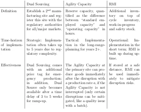
To achieve Resilience, our industrial partner focuses on three risk

mitiga-tion levers, which are under the company’s direct control (see Table 1): Dual

Sourcing, Agility Capacity, and Risk Mitigation Inventory (RMI).

To assess Supply Chain Resilience on a product level, the company sets

targets for each Resilience lever separately. The Dual Sourcing lever is

mea-sured in terms of market coverage of the Dual Source with respect to market

registrations. An Agility Capacity of 20% is targeted for the various

manu-facturing sites, and RMI is determined by covering the 95th _{percentile of a}

so-called Disruption Risk Profile (see below). The company has no

methodol-ogy in place to determine how the Resilience levers relate to one another, e.g.

to what extent RMI can be decreased in the presence of Dual Sourcing and

Agility Capacity.

The idea behind the Disruption Risk Profile is to assess a manufacturing

site’s ability to recover from a variety of operational and catastrophic events.

Such an event could be a biological contamination within the manufacturing

site, a quality issue, or a natural hazard. These events are typically rare (less

Dual Sourcing Agility Capacity RMI

Definition Establish a 2nd

manu-facturing site and reg-ister this site with the regulatory authorities for all/major markets.

Reserve capacity, quan-tified as the difference between “standard em-ployed capacity” and “operating capacity” in hours.

Additional

inven-tory on top of

cycle inventory, work-in-progress and safety stock.

Time-horizon of implemen-tation

Strategic: Implemen-tation often takes up to 5 years due to reg-ulatory complexity.

Tactical: Implementa-tion in the long-range-planning for years 2+.

Operational: Im-plementation in the short term; RMI is built up during up-time.

Effectiveness Dual Sourcing comes with an additional price tag for

emer-gency production;

in addition, Dual

Source only becomes available after a time delay of 3 to 5 weeks for ramp-up.

The Agility Capacity at the primary site can pro-duce goods immediately after the disruption with a production ratea, if the Agility Capacity is not interrupted (only certain disruptions can be miti-gated, like a quality issue with a batch).

If stored at a safe distance, RMI can be used immedi-ately to mitigate disruption risks.

can have a significant impact by causing a long disruption time (i.e. typically

longer than four weeks). As a first step, the following data is collected for all

relevant risk events that might cause supply disruptions: probability of the

event and impact in terms of length of supply disruption. Probability and

impact are determined for three scenarios: best, worst, and most likely case.

This data is based on past records, a survey with the manufacturing sites, and

commercially bought insurance data. The results are fed into a Monte Carlo

simulation leading to a so-calledDisruption Risk Profile that provides the

cu-mulative probability distribution function for the maximal disruption time in

a given year. The company has conducted this Disruption Risk Assessment

for several key sites. Given the range of input factors being considered,

man-agement has decided to cover the 95th _{percentile of aDisruption Risk Profile}

with RMI.

Based on our experience with the company, we formulate our main research

questions:

1. Can we define a holistic quantitative Resilience metric that considers

RMI and process flexibility jointly?

2. What are optimal RMI levels if process flexibility is exogenously given

in terms of Dual Sourcing and Agility Capacity?

3. How does the optimal risk mitigation strategy depend on parameters

such as disruption time and Resilience metric?

3. Literature review

Two major literature streams are relevant to our research: the managerial

and academic literature on Supply Chain Resilience, which serves as the main

disruption risk management, inventory control systems, Agility Capacity and

Dual Sourcing.

The Supply Chain Resilience literature introduces different definitions,

which we briefly summarize. A supply chain disturbance is defined as “a

foreseeable or unforeseeable event, which directly affects the usual operation

and stability of an organization or a supply chain” (Barroso et al., 2008).

These disturbances concern not only the flow of goods but also information

and financial flows. In this context, it is common to define supply chain

vul-nerability “as the incapacity of the supply chain, at a given moment, to react

to the disturbances and consequently to attain its objectives” (Azevedo et al.,

2008).

Disturbances make a supply chain more vulnerable and they might affect a

company’s performance not only in terms of direct financial losses but also in

terms of negative corporate image and loss in demand. Hendricks and Singhal

(2005a, 2005b) use an empirical approach to quantify the effect of supply

chain disruptions on the long-run stock price performance. Analyzing a period

starting one year before the disruption and lasting until two years after the

disruption, they find that the average abnormal stock return after disclosing a

supply disruption was nearly -40%. Furthermore, share price volatility, which

can be taken as an indicator of equity risk, increased by 13.50% during the

subsequent two years.

In order to address the problem of vulnerability, scholars describe the

con-cept of Resilience in the supply chain as “the ability [of a supply chain] to

re-turn to its original state or move to a new, more desirable state after being

dis-turbed” (Christopher and Peck, 2004). While risk management often focuses

on high probability, low impact operational risks, Supply Chain Resilience

of these risks is considered to be increasing because of the inter-connectivity

of global supply chain networks (WEF, 2013). A key lever for achieving

Re-silience is seen in operational risk management, which is identified as the “most

important risk domain” (van Opstal, 2007) and is the focus of this paper.

For a general overview of risk management we refer to the relevant

litera-ture. Tang (2006) presents a general overview of supply chain risk management

and mitigation strategies, whereas Dong and Tomlin (2012) provide a

litera-ture review of the operational disruption management literalitera-ture. While some

authors analyze inventory management for single systems (Moinzadeh and

Aggarwal, 1997) or multi-location systems (Schmitt et al., 2015), this paper

focuses on analyzing jointly the operational measures of RMI, Dual

Sourc-ing and Agility Capacity. The relevance of balancSourc-ing inventory and capacity

decisions is pointed out by Chopra and Sodhi (2004).

Within the operations management literature, several authors have linked

Dual Sourcing with inventory decisions, or capacity decisions with inventory

decisions under specific circumstances. On the procurement side, Tomlin

(2006) analyzes a firm that can source from two suppliers and explores

pa-rameters like reliability of the supplier and volume flexibility. This work

com-plements papers that analyze Dual Sourcing decisions, e.g. (Ramasesh et al.,

1991; Chen et al., 2012; Silbermayr and Minner, 2014; Allon and Van Mieghem,

2010; Berger et al., 2004; Ruiz-Torres and Mahmoodi, 2007; Yu at al., 2009;

Sawik, 2014). These models provide powerful tools for analyzing procurement

decisions. However, our research focuses on Dual Sourcing within the

manu-facturing process, for which the assumptions and parameters differ from the

abovementioned models. Capacity and inventory decisions under seasonal

de-mand are analyzed in (Bradley and Arntzen, 1999), where the authors use a

The propagation of disruption in a network is analyzed by Liberatore et al.

(2012). Similarly, Simchi-Levi et al. (2015) analyze supply chain robustness for

different network configurations in terms of process flexibility and inventory.

Their work is based on a two-stage robust optimization model.

The interface between operational measures and business insurance is

an-alyzed by Dong and Tomlin (2012). The authors include inventory decisions

and emergency sourcing in their model. However, some assumptions differ

from our purely operational model. Some parameters that are relevant to our

model, such as time delay and finite production rate of the Dual Source, are

not considered because of their focus on insurance policies.

While there is some academic literature on modeling disruption risks,

link-ing the three mitigation measures in the context of risk management seems to

be relatively unexplored. The need for a Resilience metric is pointed out in

various managerial journals (WEF, 2012).

4. Mathematical model

The model we present in this section assumes that the firm produces a

single product and that the production is subject to disruption risk. Such a

disruption could have an internal cause such as a biological contamination at

a productions site or an external cause such as an earthquake. To mitigate

a disruption, the firm builds up RMI and process flexibility. RMI is used to

serve unmet demand instantaneously during a potential disruption. The Dual

Source and the Agility Capacity (process flexibility) allow for production after

a disruption has occurred.

RMI is typically considered an efficient risk mitigation lever for short

are efficient risk mitigation levers because carrying excessive RMI over time is

less economical.

We assume that the primary site of a single firm is exposed to a severe

disruption of length τ during a cycle of lengthT with τ < T. The disruption

occurs with probability ω. Given the low probability for such a disruption

(ω < 5%), we assume that only one disruption occurs during a cycle. This

assumption is in line with prior literature that explicitly excludes the case

that two disruptions occur simultaneously (see, for example, Simchi-Levi et

al. (2014); Hu and Kostamis (2015); Asian and Nie (2014); and Simchi-Levi et

al. (2015), p. 7 for a discussion of this assumption). During the disruption we

assume that approximate constant demand takes place, since we are focusing

on the mature stage within the life cycle of the key product.

We develop mathematical models that analytically determine optimal RMI

levels for an exogenously given process flexibility. We choose the RMI level as

our main decision variable because this variable can most easily be adapted in

practice (operational decision). Decisions regarding process flexibility are often

of a strategic/tactical nature and are not taken solely based on a mathematical

model. For completeness, however, we provide numerical results for a specific

case that jointly evaluates optimal RMI, Dual Sourcing and Agility Capacity

decisions. Our mathematical model assumes the following:

1. The primary site of a single firm is exposed to a disruption during a

cycle, with probability ω and disruption time τ.

2. The Dual Source can produce goods in an emergency case with a

pro-duction rate d. This Dual Source only becomes available after a time

delay tD (Table 1).

after the disruption with a production rate a, if the Agility Capacity is

not interrupted.

4. For mature products, demand ξ is approximately constant during the

disruption time.

5. The proportion of backlog orders to total demand is given by ∈(0,1].

6. RMI is held decentrally in a safe location (i.e. at the next manufacturing

stage) and is thus not interrupted by the disruption.

To avoid trivial solutions, we further assume thatτ ≥tD,a < ξ, anda+d+p >

ξ. The time delay of the Dual Source (assumption 2) is due to scheduling

re-strictions and the lead time of production, including quality release. For a

pharmaceutical company this delay can easily amount to 3 to 5 weeks.

Re-garding assumption 3, the availability of the Agility Capacity depends on the

disruption type. For example, a quality issue represents a major risk in some

pharmaceutical manufacturing stages within the supply chain. For such cases,

the Agility Capacity can become a viable mitigation lever as the primary site

itself is not necessarily affected. In our mathematical models, we can always

switch off the Agility Capacity by setting the relevant parameters to zero.

Assumption 6 ensures that RMI is not destroyed by the disruption. RMI

is typically stored at the next manufacturing stage, which is geographically

distant from the possible disruption location.

4.1. Analysis of the disruption phase and Resilience metric

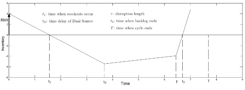
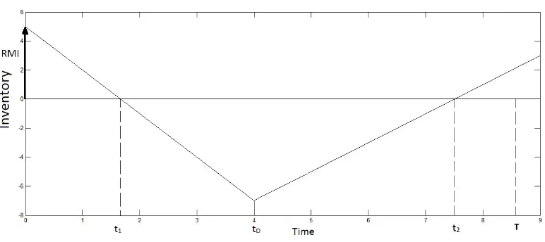
In Figure 1 we display a single disruption that takes place at time t = 0.

For a given level of RMI, we can immediately mitigate the disruption until

RMI is depleted at time t1. Starting at time tD the Dual Source produces

goods with production rate d (with d > ξ being shown in Figure 1). At time

Agility Capacity produces goods with a production rate a during t0 and t2 if

the Agility Capacity is available. The backlog ends at time t2.

Figure 1: General model showing inventory levels over time

When defining a Resilience metric, we agreed with the pharmaceutical

company that, together with the stockout quantity, the stockout time itself is

important. Rather simplistic Resilience metrics such as two separate metrics

for the relative stockout time (e.g. t1

t2, Figures 2, 3) and the projected service

level during the stockout time might not lead to satisfactory results. A metric

based on the relative stockout time might indicate a low Resilience score even

if only a few stockouts occur, spread evenly over the disruption time. Hybrid

performance measures that include stockout quantity and time have previously

been studied in the context of the service level (Schneider, 1981). Motivated

by these hybrid performance measures, we define the operational Resilience

metric ρ as

ρ= M

M +S. (1)

Figures 2, 3 for an illustration),

S =−

Z t2

t1

I(t)dt

whereI(t) is the RMI level at timet. Note thatI(t) can be negative fort > t1.

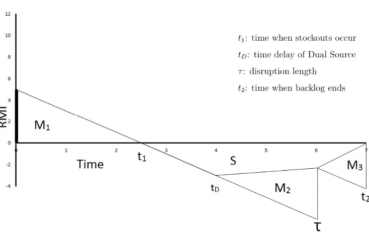
The surfaceM is the area that has been successfully mitigated (see Figures 2,

3 for an illustration).

M =M1 +M2+M3 =

Z t1

0

I(t)dt+

Z τ

tD

tddt+

Z t2

τ

t(d+p)dt,

where the first part originates from the RMI, the second part from the Dual

Source and the third part from the primary site during the recovery phase.

We have:

Lemma 1. We have: ρ ∈[0,1], dρ_dI >0, and dρ_da > dρ_dd >0. If no Dual Source

is used we have: (i) ρ = 0 iff I = 0 and (ii) ρ = 1 iff I = t2ξ. If no RMI is

held, we have: (iii) ρ= 0 iff d= 0 and (iv) ρ <1 if d=ξ.

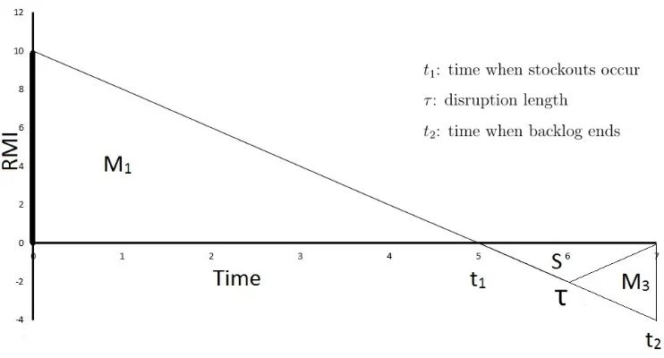
Proof. All results follow fromM = 1₂I_ξ2 + (τ−tD)2d+τ2a+ (t2−τ)2(a+d+p)

Figure 2: Stockout and mitigation surface without a Dual Source

Figures 2 and 3 illustrate that for an increased RMI or for a quicker and

stronger Dual Source, the surfaceM increases, whereas the surfaceSdecreases.

This metric is applied to the disruption time τ to visualize the company’s

capability to mitigate disruptions in a worst case scenario. Illustrative

exam-ples of the metric are presented in section 5.

To include the stockout time in our optimization problem, we define

Re-silience cost as

CR=−Rˆ

Z t2

t1

I(t)dt, (2)

with a penalty cost per item and time, ˆR. Note that RMI I(t) is negative

between timet1 and t2. This Resilience cost makes it possible to minimize the

“surface of stockouts” (area of negative inventories betweent1 andt2 in Figure

1) under further cost considerations. Such a penalty cost has been applied for

Figure 3: Stockout and mitigation surface with a Dual Source

4.2. General model

Our model is based on minimizing total costs over one cycle (e.g. one

year) for a single firm that is exposed to disruption risk. The firm decides

RMI levels before a disruption takes place. Process flexibility decisions are

exogenously given. While some cost components (reservation cost for Dual

Source and Agility Capacity) are incurred regardless of whether a disruption

occurs, other cost components are only incurred when the disruption takes

place (emergency production costs through Dual Source or Agility Capacity).

Inventory holding costs CI are only incurred as long as no disruption occurs.

Further cost parameters are: Dual Source reservation costC0

D and Dual Source

production costCD, Agility Capacity reservation costCA0 and Agility Capacity

production cost CA, a lost sales cost for stockouts CP, and a Resilience cost

The expected total cost function is

C(IG) = ˆCI(IG) + ˆCD(IG) + ˆCA(IG) +CP(IG) +CR(IG). (3)

We distinguish between two cases:

• Short time delay: tD < t1

• Long time delay: tD ≥t1

Note that t1 depends on our decision variable IG. In the following we assume

thattD < t1. At the end of this section we fully characterize this case in terms

of model parameters only. The case tD ≥t1, which follows a parallel analysis,

will be treated in the appendix. In addition, we assume that a+d < ξ. This

assumption will be relaxed in section 4.2.2.

The first cost component of Eq. 3 is the inventory holding cost, which is

incurred over the entire cycle as long as no disruption occurs.

ˆ

CI(IG) = CIIG(1−ω) (4)

whereω is the probability that a disruption occurs. Note that these inventory

holding costs are only an approximation. For a more precise treatment, one

could replace CI(1− ω) → CI(1− ω) + CIω1₂ + CIω(1− _Tτ). The CIω1₂

term reflects the situation that inventory holding costs are incurred during the

disruption time when inventory is carried for at least some of the disruption

time. TheCIω(1−_Tτ) term reflects the situation that RMI might still be held

for part of the disrupted cycle time. For simplicity, we will refer only to CI,

The Dual Source production cost consists of two components: a fixed

amount for reserving the free capacity, which is incurred over the entire cycle

regardless of whether a disruption occurs; and an additional production cost

per item that is incurred only if the disruption takes place.

ˆ

CD(IG) =CD0d+CDd(t2−tD)ω. (5)

Similarly, the Agility Capacity cost splits into two parts.

ˆ

CA(IG) =CA0a+CAat2ω. (6)

The lost sales cost is incurred for the (1−) part of the effective demand

(ξ−a−d) during the time interval (t1, τ), when lost sales occur.

ˆ

CP(IG) =CP(ξ−a−d)(1−)(τ −t1)ω. (7)

The Resilience cost consists of two parts. One part arises during the time

interval (t1, τ), before the primary site recovers. The other part originates from

the remaining backlog once the primary site recovers (time interval (τ, t2)).

CR(IG) = ˆR

Z τ−t1

0

(ξ−a−d)tdt+

Z t2−τ

0

(n+ (ξ−a−d−p)t)dtω, (8)

where n is the backlog at time τ,

The starting time of stockouts t1 is given by setting supply volumes equal to

demand volumes.

IG+at1+ (t1−tD)d=ξt1,

which becomes

t1 =

IG−dtD

ξ−a−d. (9)

The time when the backlog ends, t2, consists of two components. One is the

disruption time τ and the other is the time to serve all outstanding backlogs

once the site has recovered.

t2 =τ +

n

a+d+p−ξ. (10)

Our general model gives an explicit analytic expression for the optimal

RMI level I_G∗ depending on Dual Sourcing and Agility Capacity parameters.

Using first and second order conditions for the expected total costs (Eq. 3)

leads to

I

=

(1−ω)

ω +CP(1−)+

CAa+_CDd

a+d+p−ξ + ˆR(

(ξ−a−d)(τ−_tD)

a+d+p−ξ +τ+ dtD ξ−a−d) ˆ

R(_a+d+p−ξ+_ξ−a1_−d)

.

(11)

Note that ˆR < CI (1−ω)

ω −CP(1−)−CAa

+_CDd

a+d+p−ξ

(ξ−_aa₊−_dd₊)(_pτ₋−_ξtD)+τ would result in negative optimal RMI levels. Note further that the condition tD < t1 (short time delay) is satisfied

if and only if

−CI(1−_ωω)+CP(1−)+CAa

+_CDd

a+d+p−ξ + ˆR(

(ξ−a−d)(τ−_tD)

a+d+p−ξ +τ+ dtD ξ−a−d) ˆ

R(_a+d+p−ξ+_ξ−a1_−d)(ξ−a)

> t

.

(12)

We find in general:

CI(1 −ω)

ω −CP(1−)−

CAa+_CDd

a+d+p−ξ

(ξ−_aa₊−_dd₊)(_pτ₋−_ξtD)+τ , and for an exogenously given process flexibility, the

optimal RMI I_G∗ is given by

I_G∗ =

      

−CI(1 −ω)

ω +CP(1−)+CAa

+_CDd

a+d+p−ξ+ ˆR(

(ξ−a−d)(τ−_tD)

a+d+p−ξ +τ+ξ−dtDa−d) ˆ

R(_a+d+p−ξ+_ξ−a1_−d) for short time delay

−CI(1 −ω)

ω +CP(1−)+CAa

+_CDd

a+d+p−ξ+ ˆR(

(ξ−a)_tD+(ξ−a−d)(τ−_tD)

a+d+p−ξ +τ) ˆ

R(_a+d+p−ξ+_ξ−1_a) for long time delay.

(13)

Proof. We refer to Appendix B for the case long time delay.

Numerical results and managerial insights are discussed in section 5. In

collaboration with the pharmaceutical company we reached the conclusion that

the following two cases are relevant for applications:

• Hot Standby case: the Dual Source is strong and the disruption ends

before the primary site restarts production (a+d > ξ).

• Quick Recovery case: the disruptions ends immediately once the primary

site starts producing goods again. This is relevant for applications in

which large batch sizes are produced (e.g. the production of the Active

Pharmaceutical Ingredient, API) and it is reasonable to assume that

p→ ∞.

In the following we discuss these two cases.

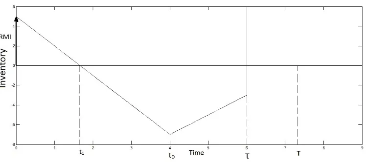
4.2.1. Hot Standby case

Here we address the special case that the Dual Source is strong and the

disruption ends before the primary site recovers, a+d > ξ (see Figure 4).

This can be the case, for example, when the Dual Source has sufficient excess

Figure 4: Hot Standby case: Dual Source/Agility Capacity takes over full production

The analysis of this case is similar to the general model. However, in

contrast to Proposition 1, we only have to consider the case long time delay

because the sum of the Dual Source and Agility Capacity production rates

is assumed to be greater than the demand rate. Hence, stockouts only occur

before the Dual Source starts production. Analogous to Proposition 1, the

starting time of stockouts t1 is given by

t1 =

IH

ξ−a, (14)

where IH is the RMI level. The maximal backlog n is given by

n = (ξ−a)(tD−t1)= ((ξ−a)tD−IH),

which leads to

t2 =

n

a+d−ξ +tD =

(ξ−a)tD−IH

Similar to the general model, we find:

Proposition 2. For a positive Resilience cost per item and per time Rˆ ≥

CI(1 −ω)

ω −CP(1−)−CAa

+_CDd

a+d−ξ

tD(1+_a+ξ−_d−a_ξ) , and for an exogenously given process flexibility, the

optimal RMI I_H∗ is given by

I_H∗ =tD(ξ−a)−

CI(1

−ω)

ω −CP(1−)−

CAa+CDd a+d−ξ ˆ

R(_ξ−1_a+ _a+d−ξ) . (16)

Proof. See Appendix C for a detailed proof.

Note that for ˆR→ ∞ we have

I_H∗ =tD(ξ−a), (17)

which means that there is sufficient RMI to cover the whole disruption until

the Dual Source is qualified.

4.2.2. Quick Recovery case

In this case we assume that there are no more stockouts or backlogs once

the primary site is fully functional again (see Figure 5). In the pharmaceutical

industry this is the case, for example, when large batch sizes (e.g. API) are

produced.

For the general case we can take the limit p→ ∞and find:

Proposition 3. For a positive Resilience cost per item and per time Rˆ ≥

CI(1 −ω)

ω −CP(1−)

τ , and for an exogenously given process flexibility, the optimal

RMI I_Q∗ is given by

I_Q∗ =

  

 

(−CI(1−_ωω)+CP(1−)+ ˆR(τ+_ξ−dtDa−d))(ξ−a−d) ˆ

R for short time delay

(−CI(1 −ω)

ω +CP(1−)+ ˆRτ)(ξ−a) ˆ

R for long time delay

Figure 5: Quick Recovery case: Strong primary site

Proof. See Appendix D for a proof.

Note that the condition tD < t1 (short time delay) is satisfied if and only

if

−CI

(1−ω)

ω +CP(1−) + ˆRτ ˆ

R > tD. (19)

5. Numerical results

In this section we explore how different model parameters influence the risk

mitigation strategy. First, we provide an illustration of the Resilience metric.

Second, we analyze RMI and process flexibility decisions jointly. Third, we

perform a sensitivity analysis of our decision variable in relevant model

pa-rameters.

5.1. Definition of metric

We recall that the Resilience metric ρ is defined by stockout quantity and

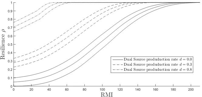
stockout time. In Figure 6 we provide an illustrative visualization of the metric

of our resilience metric ρ (y-axis) depending on RMI (x-axis) for the Quick

Recovery case. There are three groups of lines for the different Dual Sourcing

scenarios (d= 0.0, d = 0.3, d= 0.8). Each group contains three lines for the

different Agility Capacity scenarios (a = 0.00, a = 0.05, a = 0.10). The plot

is based on the following further parameters: τ = 210, tD = 30, ξ = 1, d =

0.0, 0.3, 0.8, a= 0.00, 0.05, 0.10, = 1.

Figure 6 illustrates the extent to which RMI can be reduced if disruptions

are mitigated through Dual Sourcing and/or Agility Capacity if ρ is kept

constant. For example, at ρ= 0.8, RMI can decrease from RM I = 140 units

(no Dual Source or Agility Capacity) to RM I = 7 units (d = 0.8, a = 0.10).

The graph also illustrates how Resilience ρ increases if Dual Sourcing and/or

Agility Capacity increase while RMI is kept constant. For example, atRM I =

50 units, Resilience increases fromρ= 0.1 (no Dual Source or Agility Capacity)

toρ= 1.0 (d= 0.8,a= 0.10).

RMI

0 20 40 60 80 100 120 140 160 180 200

R

es

il

ie

n

ce

ρ

0 0.1 0.2 0.3 0.4 0.5 0.6 0.7 0.8 0.9 1

Dual Source produduction rated= 0.0

Dual Source produduction rated= 0.3

Dual Source produduction rated= 0.8

5.2. Variable target Resilience ρ

So far we have considered the Dual Source production rate d to be

exoge-nously given. In this section we minimize the total cost function (D.1) for

the Quick Recovery case whereby we keep IQ and d as independent decision

variables and a as exogenously given:

C(IQ, d) = ˆCI(IQ) + ˆCD(IQ, d) + ˆCA(IQ) +CP(IQ, d) +CR(IQ, d). (20)

We perform the numerical optimization with the fmincon solver from

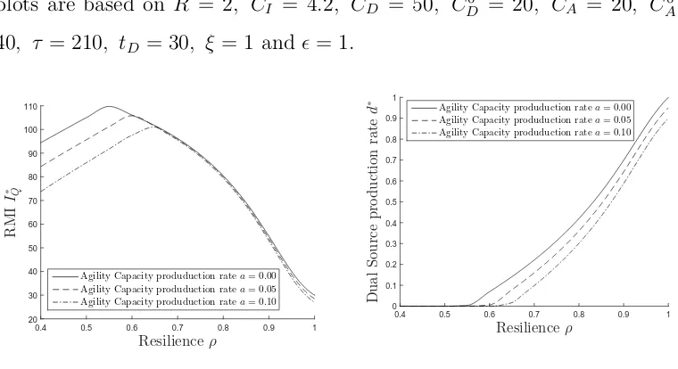
MAT-LAB. Figure 7 shows how RMI I_Q∗ (y-axis) depends on the target Resilience

ρ (x-axis). Likewise, Figure 8 shows how the Dual Source production rate

d∗ (y-axis) depends on the target Resilience ρ (x-axis). In both figures we

display three plots for different Agility Capacity production rates respectively

(a = 0.00, a = 0.05, a = 0.10). Figure 7 illustrates that RMI increases in

Resilience ρ for ρ < 0.55, before the RMI reaches its maximum value in the

range 0.55< ρ < 0.65 (depending on Agility Capacity production rate a).

Af-terwards RMI decreases in ρ as the Dual Source production rate d∗ increases

(Figure 8). Note that RMI does not decrease to 0 when the Dual Source covers

100% of the demand (d= 1.0) and whenρ= 1.0 due to the time delay of the

Dual Source.

In Figure 7, for ρ < 0.65, RMI levels decrease in the Agility Capacity

production rate a. For ρ >0.65, RMI hardly changes in the Agility Capacity

production rate. However, forρ >0.65, Dual Sourcing decreases in the Agility

Capacity production ratea, revealing that Agility Capacity and Dual Sourcing

are substitutes (Figure 8). It appears that RMI and Agility Capacity are

substitutes as long as no Dual Source is available. Once the Dual Source is

plots are based on ˆR = 2, CI = 4.2, CD = 50, CD0 = 20, CA = 20, CA0 =

40, τ = 210, tD = 30, ξ = 1 and= 1.

Resilienceρ

0.4 0.5 0.6 0.7 0.8 0.9 1

R M I I ∗ Q 20 30 40 50 60 70 80 90 100 110

Agility Capacity produduction ratea= 0.00

Agility Capacity produduction ratea= 0.05

Agility Capacity produduction ratea= 0.10

Figure 7: RMI depending on Resilience metric

Resilienceρ

0.4 0.5 0.6 0.7 0.8 0.9 1

D u al S ou rc e p ro d u ct ion rat e d ∗ 0 0.1 0.2 0.3 0.4 0.5 0.6 0.7 0.8 0.9 1

Agility Capacity produduction ratea= 0.00 Agility Capacity produduction ratea= 0.05 Agility Capacity produduction ratea= 0.10

Figure 8: Dual Source production rate de-pending on Resilience metric

Following prior literature (for example, Tomlin (2006) and the literature

cited therein), this numerical example does not consider fixed costs for the

Dual Source. There are, however, two ways to incorporate such fixed costs

for practical applications. One can either set an additional constraint on d

(e.g. d > 0.05) or one can perform an additional NPV calculation (e.g. the

discounted cash flow is calculated for each cycle minus the investment costs

for the Dual Source) and then evaluate the value of Dual Sourcing.

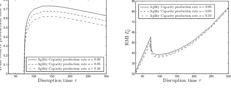
5.3. Variable disruption time τ

As in section 5.2 we minimize the total cost function (D.1) for the Quick

Recovery case whereby we keep IQ and d as independent decision variables

and a as exogenously given. However, we keep ρ= 0.9 constant and vary the

disruption time τ. All other parameters are as above. Figure 9 shows that the

Dual Source is only used for a minimal disruption time τ = 74. For shorter

the inventory holding costs. For τ > 74 the Dual Source production rate d∗

increases in τ until a maximum is reached at τ = 150. Interestingly, d∗

de-creases in τ for long disruption times. One might expect that long disruption

times are optimally mitigated with a large Dual Source production rate. We

recall that two cost components are associated with the Dual Source: a

reser-vation fee C0

Dd, and an emergency production cost CDd(t2 −tD)ω. As there

is an extra price tag for emergency production through the Dual Source, Dual

Sourcing may not be the optimal strategy for long disruption timesτ. Instead,

holding RMI over all the time may be cheaper than paying this extra price tag

for emergency production.

Figure 10 shows that RMI increases in τ for τ <74. Forτ > 74, the Dual

Source is in use and RMI I_Q∗ decreases in τ. As a∗ decreases in τ for long

disruption times, RMI increases in τ as ρ is kept constant.

50 100 150 200 250 300 0 0.1 0.2 0.3 0.4 0.5 0.6 0.7 0.8

Disruption timeτ

D u a l S o u rc e p ro d u ct io n ra te d ∗

Agility Capacity production ratea= 0.00 Agility Capacity production ratea= 0.05 Agility Capacity production ratea= 0.10

Figure 9: Dual Source production rate de-pending on disruption time

50 100 150 200 250 300 20 30 40 50 60 70 80 90

Disruption timeτ

R

M

I

I

∗ Q

Agility Capacity production ratea= 0.00 Agility Capacity production ratea= 0.05 Agility Capacity production ratea= 0.10

Figure 10: RMI depending on disruption time

5.4. Sensitivity analysis

We perform a sensitivity analysis in the optimal RMI I_G∗ for the

results follow directly from Eq. (13). For the sensitivity in τ note that

dI_G∗

dτ ≥ (ξ −a−d) > 0. As the probability for a disruption increases or as

the disruption time increases, more RMI is built up. Likewise, if Dual

Sourc-ing/Agility Capacity costs or penalty costs increase, RMI increases as well.

RMI decreases in the inventory holding costs. I_G∗ may decrease or increase in

ˆ

R. For short time delay we have: dIG∗ dRˆ = −

1 ˆ R2

−CI(1−_ωω)+CP(1−)+CAa

+_CDd

a+d+p−ξ

(

a+d+p−ξ+

1

ξ−a−d)

. The

sign of the last term is ambiguous. Depending on the cost parameters, it could

be that Dual Sourcing/Agility Capacity is more efficient than RMI as ˆR

in-creases. Regarding the sensitivity inξ,d,a,p,tD and, we refer to the relevant

Quick Recovery case (tD < t1) as the economic insights can best be studied for

this case: RMI increases in the Dual Source time delay tD ( dI∗

Q

dtD =d > 0). As

the time delay of the Dual Source increases, RMI increases by an amount that

is proportional to the production rate of the Dual Source. For the sensitivity

in the proportion of backlog orders to total demand, we find a sensitivity to

the power of −2: dI

∗ Q

d =

CI1−ωω−CP ˆ

R2 (ξ−a−d). The sensitivity in the demand

rate or production rate of Dual Source/Agility Capacity is given by: dI

∗ Q

dξ =

−CI1−ωω+CP(1−) ˆ

R +τ,

dI∗ Q

dd =

CI1−ωω−CP(1−) ˆ

R −τ +tD,

dI∗ Q

da =

CI1−ωω−CP(1−) ˆ

R −τ.

The sensitivity of I_Q∗ in the last four parameters is ambiguous. Depending

on penalty costs, inventory holding costs, disruption probabilities, disruption

times and proportion of backlog orders to total demand, I_Q∗ may increase or

decrease in the last parameters.

6. Conclusions and future research

In this research we have analyzed the three risk mitigation strategies RMI,

Dual Sourcing and Agility Capacity. We find analytic results for optimal

RMI levels if the characteristics for Dual Sourcing and Agility Capacity are

to track Supply Chain Resilience and assess trade-offs between risk mitigation

levers in quantitative terms. This metric is based on the stockout time as well

as the percentage of served demand during the disruption time. Our numerical

results suggest that RMI and Agility Capacity can be substitutes as long as no

Dual Source is available. Once the Dual Source is available, Agility Capacity

and Dual Sourcing appear to be substitutes. We further show that for long

disruption times, the optimal Dual Source production rate may decrease in

the disruption time.

Our modeling work was validated by our industrial partner and

subse-quently applied to Supply Chain Resilience assessments for life-saving drugs.

Single and Dual Sourcing scenarios (with and without Agility Capacity) were

analyzed for the production in various production stages.

While these models are based on the practice and structure of a

pharma-ceutical supply chain, this work raises a couple of research questions to explore

the generality of the analysis and the results across industries. It would be

interesting to study if these results still hold under stochastic demand. This

would also allow to explore the relation of RMI to safety stock in the context

of the (Q, R) model. Further research extensions could address multi-echelon

supply chains. In the pharmaceutical industry this would entail analyzing drug

substance, drug product and finished goods production holistically.

Acknowledgments

The authors are grateful to the editors and anonymous reviewers for

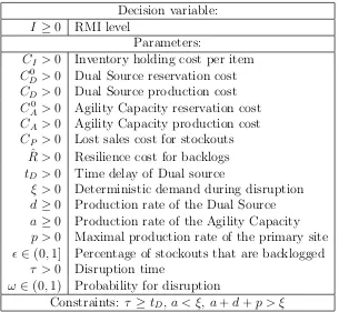
Appendix A. Decision variable and parameters of the model

Decision variable: I ≥0 RMI level

Parameters:

CI >0 Inventory holding cost per item

C_D0 >0 Dual Source reservation cost CD >0 Dual Source production cost

C0

A>0 Agility Capacity reservation cost

CA>0 Agility Capacity production cost

CP >0 Lost sales cost for stockouts ˆ

R > 0 Resilience cost for backlogs tD >0 Time delay of Dual source

ξ > 0 Deterministic demand during disruption d≥0 Production rate of the Dual Source a ≥0 Production rate of the Agility Capacity p > 0 Maximal production rate of the primary site ∈(0,1] Percentage of stockouts that are backlogged

τ > 0 Disruption time

ω∈(0,1) Probability for disruption

Constraints: τ ≥tD,a < ξ,a+d+p > ξ

Appendix B. Proof of Proposition 1

Proof. For the caselong time delay we have to consider the following changes:

The lost sales cost for stockouts consists of two parts. One part arises during

the time interval (t1, tD), before the Dual Source delivers goods. The other

part arises during the time interval (tD, τ).

ˆ

CP(IG) = CP(1−)

(ξ−a)(tD −t1) + (ξ−a−d)(τ −tD)

ω. (B.1)

The Resilience cost consists of three parts. One part arises during the time

interval (t1, tD), before the Dual Source delivers goods. Another part arises

during the time interval (tD, τ). The third part originates from the remaining

backlog once the primary site recovers (time interval (τ, t2)).

CR(IG) = Rˆ

Z tD−t1

0

(ξ−a)tdt+

Z τ−tD

0

((ξ−a)tD −IG+ (ξ−a−d)t)dt

+

Z t2−τ

0

(n+ (ξ−a−d−p)t)dtω, (B.2)

where n is the backlog at time τ,

n= [(ξ−a)tD + (ξ−a−d)(τ−tD)−IG].

The starting time of stockouts t1 is given by setting supply volumes equal to

demand volumes.

IG+at1 =ξt1,

which becomes

t1 =

IG

The time when the backlog ends, t2, consists of two components. One is the

disruption time τ and the other is the time to serve all outstanding backlogs

once the site has recovered.

t2 =τ +

n

a+d+p−ξ. (B.4)

Using first and second order conditions for the expected total costs (Eq.

3) leads to

I

=

(1−ω)

ω +CP(1−)+

CAa+_CDd

a+d+p−ξ + ˆR(

(ξ−a)_tD+(ξ−a−d)(τ−_tD)

a+d+p−ξ +τ) ˆ

R(_a+d+p−ξ+_ξ−1_a)

.

(B.5)

Regarding the second order condition, it is sufficient to look at the Resilience

cost because the other terms of the objective function are linear in IG:

∂CR

∂IG

=−Rˆ (ξ−a)(tD−t1)+(ξ−a−d−p)(t2−τ)

−

a+d+p−ξ−

2n a+d+p−ξ

∂2CR

∂I2 G

= Rˆ (ξ−a) 1

(ξ−a)+ (ξ−a−d−p)

−

a+d+p−ξ

2

+ 2

2

a+d+p−ξ

= Rˆ +

2

a+d+p−ξ >0.

Appendix C. Direct proof of Proposition 2

Proof. The proof is based on minimizing the total cost function

The first cost component is the inventory holding cost.

ˆ

CI(IH) =CIIH(1−ω). (C.2)

The Dual Source production cost consists of a fixed component for reserving

the free capacity and an additional production cost per item.

ˆ

CD(IH) = CD0d+CDd(t2−tD)ω. (C.3)

Similarly, the Agility Capacity cost is given by

ˆ

CA(IH) =CA0a+CAat2ω. (C.4)

The lost sales cost for stockouts is given by

ˆ

CP(IH) = CP(ξ−a)(1−)(tD−t1)ω. (C.5)

The Resilience cost is given by

CR(IH) = ˆR

Z t2−τ

0

(n+ (ξ−a−d)t)dt+

Z τ−t1

0

(ξ−a−d)tdt

ω, (C.6)

where n is the backlog at time τ,

n = (ξ−a)(tD−t1)= ((ξ−a)tD−IH).

t1 is given by

t1 =

IH

Using first and second order constraints leads to

I_H∗ = −CI

(1−ω)

ω +CP(1−) +

CAa+CDd

a+d−ξ + ˆRtD(1 + ξ−a a+d−ξ) ˆ

R(_ξ−1_a +_a+d−ξ) (C.7)

= tD(ξ−a)−

CI(1

−ω)

ω −CP(1−)−

CAa+CDd a+d−ξ ˆ

R(_ξ−1_a+ _a+d−ξ) . (C.8)

Appendix D. Direct proof of Proposition 3

Proof. The proof is based on minimizing the total cost function

C(IQ) = ˆCI(IQ) + ˆCD(IQ) + ˆCA(IQ) +CP(IQ) +CR(IQ). (D.1)

The first cost component is the inventory holding cost.

ˆ

CI(IQ) =CIIQ(1−ω). (D.2)

The Dual Source production cost consists of a fixed component for reserving

the free capacity and an additional production cost per item.

ˆ

CD(IQ) =CD0d+CDd(τ −tD)ω. (D.3)

Similarly, the Agility Capacity cost is given by

ˆ

The lost sales cost for stockouts is given by

ˆ

CP(IQ) =



 

 

CP(1−)(ξ−a−d)(τ −t1)ω for short time delay

CP(1−)

(ξ−a)(tD−t1) + (ξ−a−d)(1−)(τ−tD)

ω for long time delay.

(D.5)

The Resilience cost is given by

CR(IQ) =

     ˆ

RRτ−t1

0 (ξ−d−a)tdt

ω forshort time delay

ˆ

RRtD−t1

0 (ξ−a)tdt+ Rτ−tD

0 (m+ (ξ−d−a)t)dt

ω forlong time delay,

(D.6)

where the backlogm at timetD is given by:

m= ((ξ−a)tD −IQ).

t1 is given by

t1 =

  

 

IQ−dtD

ξ−a−d for short time delay

IQ

ξ−a for long time delay.

(D.7)

Using first and second order constraints leads to

I_Q∗ =

  

 

(−CI(1−_ωω)+CP(1−)+ ˆR(τ+_ξ−dtD_a−d))(ξ−a−d) ˆ

R for short time delay

(−CI(1−_ωω)+CP(1−)+ ˆRτ)(ξ−a) ˆ

R for long time delay.

(D.8)

Appendix E. Calculation of Resilience metric

To illustrate how to calculate ρ we provide an example with RM I = 105,

d = 0.0 and a = 0.00: M = M1 =

Rt1

0 I(t)dt =

Rt1

0 RM I −ξtdt = RM I ∗

t1 − 1₂ξ∗t21 = 5512.5 with t1 = RM I_ξ = 105 and S =−

Rt2

t1 I(t)dt =

Rt2

ξ1

2(t2−t1)

2 _{= 5512.5 leading toρ=} M

References

Allon, G., & Van Mieghem, J.A. (2010). Global Dual Sourcing: Tailored

Base-surge Allocation to Near- and Offshore Production. Management Science,

56 (1), 110-124.

Asian, S., & Nie, X. (2014). Coordination in Supply Chains with Uncertain

Demand and Disruption Risks: Existence, Analysis, and Insights. IEEE

Transactions on Systems, Man, and Cybernetics: Systems, 44, 9.

Azevedo, S.G., Carvalho, H., & Cruz-Machado, V. (2008). Supply Chain

Vul-nerability: Environment Changes and Dependencies. International Journal

of Logistics and Transport, 1, 41–55.

Axs¨ater, S. (2006). Inventory Control. Springer, New York, USA.

Barroso, A.P., Machado, V.H., & Cruz Machado, V. (2008). A Supply Chain

Disturbances Classification.Proceedings of the International Conference on

Industrial Engineering and Engineering Management, ISBN 9781424426294,

Singapore, December.

Berger, P.D., Gerstenfeld, A., & Zeng, A.Z. (2004). How Many Suppliers Are

Best? A Decision-Analysis Approach.Omega, 32, 9-15.

Bradley, J.R., & Arntzen, B.C. (1999). The Simultaneous Planning of

Pro-duction, Capacity, and Inventory in Seasonal Demand Environments.

Oper-ations Research, 47, 795–806.

Chen, J., Zhao, X., & Zhou, Y. (2012). A Periodic-Review Inventory System

with a Capacitated Backup Supplier for Mitigating Supply Disruptions.

Chopra, S., & Sodhi, M.S. (2004). Managing Risk to Avoid Supply-Chain

Breakdown. MIT Sloan Management Review, 46, 52-62.

Christopher, M., & Peck, H. (2004). Building the Resilient Supply Chain.The

International Journal of Logistics Management, 15, 1-13.

Dong, L., & Tomlin, B. (2012). Managing Disruption Risk: The Interplay

Between Operations and Insurance.Management Science, 58, 1898–1915.

Government Accountability Office (GAO). (2014). DRUG SHORTAGES

Pub-lic Health Threat Continues, Despite Efforts to Help Ensure Product

Avail-ability. Report to Congressional Addressees. GAO-14-194, http://www.

gao.gov/products/GAO-14-194

Hendricks, K.B., & Singhal, V.R. (2005a). An Empirical Analysis of the Effect

of Supply Chain Disruptions on Long-Run Stock Price Performance and

Equity Risk of the Firm.Production and Operations Management, 14, 35–52.

Hendricks, K.B., & Singhal, V.R. (2005b). Association Between Supply Chain

Glitches and Operating Performance. Management Science, 51, 695–711.

Hu, B., & Kostamis, D. (2015). Managing Supply Disruptions when Sourcing

from Reliable and Unreliable Suppliers.Production and Operations

Manage-ment, 24, 5, 808-820.

Liberatore, F., Scaparra, M.P. & Daskin, M.S. (2012). Optimization Methods

for Hedging Against Disruptions with Ripple Effects in Location Analysis.

Omega, 40(1), 21-30.

Moinzadeh, K., & Aggarwal, P. (1997). Analysis of a Production/Inventory

System Subject to Random Distributions. Management Science, 43,

Ramasesh, R.V., Ord, J.K., Hayya, J.C., & Pan, A. (1991). Sole Versus Dual

Sourcing in Stochastic Lead-Time (s, Q) Inventory Models. Management

Science, 37, 428-443.

Sawik, T. (2014). Joint supplier selection and scheduling of customer orders

under disruption risks: Single vs. dual sourcing. Omega, 43, 83-95.

Ruiz-Torres, A.J., & Mahmoodi, F. (2007). The Optimal Number of Suppliers

Considering the Costs of Individual Supplier Failures.Omega, 35, 104-115.

Schmitt, A.J., Sun, S.A., Snyder, L.V., & Shen, Z.J.M. (2015).

Centraliza-tion versus DecentralizaCentraliza-tion: Risk Pooling, Risk DiversificaCentraliza-tion, and Supply

Uncertainty in a One-Warehouse Multiple-Retailer System.Omega, 52,

201-212.

Schneider, H. (1981). Effect of Service-Levels on Order Points or Order-Levels

in Inventory Models. International Journal of Production Research, 19,

615–631.

Schweizer Radio und Fernsehen. (2014).http://www.srf.ch/news/schweiz/

medikamentenmangel-meldepflicht-soll-nachschub-sichern.

Seifert, R. W., & L¨ucker, F. (2014). The Five Pillars of Supply Chain

Re-silience: How Companies Implement Resilience in Their Supply Chains.

IMD – Tomorrow’s Challenges, 44, June.

Simchi-Levi, D., Schmidt, W., & Wei, Y. (2014). From Superstorms to Factory

Fires: Managing Unpredictable Supply-Chain Disruptions. Harvard

Busi-ness Review, January-February.

Simchi-Levi, D., Wang, H., & Wei, Y. (2015). Increasing Supply Chain

Silbermayr, L., & Minner, S. (2014). A Multiple Sourcing Inventory Model

under Disruption Risk.International Journal of Production Economics, 149,

37-46.

Sodhi, M. S., & Tang, C. S. (2012). Managing Supply Chain Risk.International

Series in Operations Research & Management Science, 172, Springer, New

York.

Tang, C.S. (2006). Perspectives in Supply Chain Risk Management.

Interna-tional Journal of Production Economics, 103 (2), 2006, 451-488.

Tomlin, B. (2006). On the Value of Mitigation and Contingency Strategies for

Managing Supply Chain Disruption Risks. Management Science, 52,

639-657.

van Opstal, D. (2007). Transform. The Resilient Economy: Integrating

Com-petitiveness and Security. Council on Competitiveness, United States of

America.

World Economic Forum, (2012). New Models for Addressing Supply Chain

and Transport Risk.Industry Agenda.

World Economic Forum, (2013). Building Resilience in Supply Chains.

Indus-try Agenda.

Yu, H., Zeng, A., & Zhao, L. (2009). Single or Dual Sourcing: Decision-Making