Class imbalance ensemble learning based on the margin theory

(1)

sciences

Article

Class Imbalance Ensemble Learning Based on the

Margin Theory

Wei Feng1,*ID_{, Wenjiang Huang}1_{and Jinchang Ren}2

1 _{Key laboratory of Digital Earth Science, Institute of Remote Sensing and Digital Earth,}

Chinese Academy of Sciences, Beijing 100094, China; [email protected]

2 _{Department of Electronic and Electrical Engineering, University of Strathclyde, Glasgow G1 1XW, UK;}

[email protected]

* Correspondence: [email protected]; Tel.: +86-138-9575-1095

Received: 10 April 2018; Accepted: 14 May 2018; Published: 18 May 2018

Abstract:The proportion of instances belonging to each class in a data-set plays an important role in machine learning. However, the real world data often suffer from class imbalance. Dealing with multi-class tasks with different misclassification costs of classes is harder than dealing with two-class ones. Undersampling and oversampling are two of the most popular data preprocessing techniques dealing with imbalanced data-sets. Ensemble classifiers have been shown to be more effective than data sampling techniques to enhance the classification performance of imbalanced data. Moreover, the combination of ensemble learning with sampling methods to tackle the class imbalance problem has led to several proposals in the literature, with positive results. The ensemble margin is a fundamental concept in ensemble learning. Several studies have shown that the generalization performance of an ensemble classifier is related to the distribution of its margins on the training examples. In this paper, we propose a novel ensemble margin based algorithm, which handles imbalanced classification by employing more low margin examples which are more informative than high margin samples. This algorithm combines ensemble learning with undersampling, but instead

of balancing classes randomly such as UnderBagging, our method pays attention to constructing

higher quality balanced sets for each base classifier. In order to demonstrate the effectiveness of the

proposed method in handling class imbalanced data,UnderBaggingandSMOTEBaggingare used in a

comparative analysis. In addition, we also compare the performances of different ensemble margin definitions, including both supervised and unsupervised margins, in class imbalance learning.

Keywords:classification; ensemble margin; imbalance learning; ensemble learning; multi-class

1. Introduction

Class distribution, i.e., the proportion of instances belonging to each class in a data set, plays a key role in any kind of machine-learning and data-mining research. However, the real world data often suffer from class imbalance. The class imbalance case has been reported to exist in a wide variety

of real-world domains, such as face recognition [1], text mining [2], software defect prediction [3],

and remote sensing [4]. Binary imbalanced data classification problems occur when one class, usually

the one that refers to the concept of interest (positive or minority class), is underrepresented in the data-set; in other words, the number of negative (majority) instances outnumbers the amount of

positive class instances [5–7]. Processing minority class instances as noise can reduce classification

accuracy. Dealing with multi-class tasks with different misclassification costs of classes is harder

than dealing with two-class ones [8–10]. Some traditional classification algorithms, such as K-Nearest

Neighbors (KNN), Support Vector Machines (SVM), and decision trees, which show good behavior in problems with balanced classes, do not necessarily achieve good performance in class imbalance

(2)

problems. Consequently, how to classify imbalanced data effectively has emerged as one of the biggest challenges in machine learning.

The objective of imbalance learning can be generally described asobtaining a classifier that will

provide high accuracy for the minority class without severely jeopardizing the accuracy of the majority class. Typically, there are four methods for imbalanced learning [11]: sampling methods [12],

cost-sensitive methods [7,13], kernel-based methods [7] and active learning methods [14].

• Sampling methods: The objective of these non-heuristic methods is to provide a balanced distribution by considering the representative proportions of class examples. They are carried out

before training starts. These methods will be presented in detail in Section2.1.

• Cost-sensitive methods: These methods incorporate both data level transformations (by adding costs to instances) and algorithm level modifications (by modifying the learning process to accept costs). They generally use the cost matrix to consider the costs associated with misclassifying

samples [11]. Cost-sensitive neural network [15] with threshold-moving technique was proposed

to adjust the output threshold toward inexpensive classes, such that high-cost samples are unlikely to be misclassified. Three cost-sensitive methods, AdaC1, AdaC2, and AdaC3 were

proposed [16] and cost items were used to weight the updating strategy in the boosting algorithm.

The disadvantage of these approaches is the need to define misclassification costs, which are not

usually available in the data sets [5].

• Kernel-based methods: The principles of kernel-based learning are centered on the theories

of statistical learning and Vapnik-Chervonenkis dimensions [17,18]. In kernel-based methods,

there have been many works to apply sampling and ensemble techniques to the support vector

machine (SVM) concept [19]. Different error costs [20] were suggested for different classes to bias

the SVM to shift the decision boundary away from positive instances and make positive instances more densely distributed.

• Active learning methods: Traditional active learning methods were used to solve the imbalanced training data problem. Recently, various approaches on active learning from imbalanced data

sets were proposed [14]. Active learning effectively selects the instances from a random set of

training data, therefore significantly reducing the computational costs when dealing with large imbalanced data sets. The major drawback of these approaches is large computation costs for

large datasets [14].

Ensemble classifiers are known to increase the accuracy of single classifiers by combining several of

them and have been successfully applied to imbalanced data-sets [21–24]. Ensemble learning methods

have been shown to be more effective than data sampling techniques to enhance the classification

performance of imbalanced data [25]. However, as the standard techniques for constructing ensembles

are rather too overall accuracy oriented, they still have difficulty sufficiently recognizing the minority

class [26]. So, the ensemble learning algorithms have to be designed specifically to effectively handle

the class imbalance problem [5]. The combination of ensemble learning with imbalanced learning

techniques (such as sampling methods presented in Section2.1) to tackle the class imbalance problem

has led to several proposals in the literature, with positive results [5]. Hence, aside from conventional

categories such as kernel-based methods, ensemble-based methods can be classified into a new category

in imbalanced domains [5]. In addition, the idea of combining multiple classifiers itself can reduce the

probability of overfitting.

Margins, which were originally applied to explain the success of boosting [27] and to develop the

Support Vector Machines (SVM) theory [17], play a crucial role in modern machine learning research.

The ensemble margin [27] is a fundamental concept in ensemble learning. Several studies have shown

that the generalization performance of an ensemble classifier is related to the distribution of its margins

on the training examples [27]. A good margin distribution means that most examples have large

margins [28]. Moreover, ensemble margin theory is a proven effective way to improve the performance

(3)

margin values, and thus help ensemble classifiers to avoid the negative effects of redundant and noisy

samples. In machine learning, the ensemble margin has been used in imbalanced data sampling [21],

noise removal [30–32], instance selection [33], feature selection [34] and classifier design [35–37].

In this paper, we propose a novel ensemble margin based algorithm, which handles imbalanced classification by employing more low margin examples which are more informative than high margin samples. This algorithm combines ensemble learning with undersampling, but instead of balancing

classes randomly such as UnderBagging [38], our method pays attention to constructing higher quality

balanced sets for each base classifier. In order to demonstrate the effectiveness of the proposed

method in handling class imbalanced data, UnderBagging [38] and SMOTEBagging [8], which will be

presented in detail in the following section, are used in a comparative analysis. We also compare the performances of different ensemble margin definitions, including the new margin proposed, in class imbalance learning.

The remaining part of this paper is organized as follows. Section2presents an overview of

the imbalanced classification domain from the two-class and multi-class perspectives. The ensemble margin definition and the effect of class imbalance on ensemble margin distribution is presented

in Section 3. Section 4 describes in detail the proposed methodology. Section 5 presents the

experimental study and Section 6provides a discussion according to the analysis of the results.

Finally, Section7presents the concluding remarks.

2. Related Works

2.1. Sampling Methods for Learning from Imbalanced Data

The sampling approach rebalances the class distribution by resampling the data space. This method avoids the modification of the learning algorithm by trying to decrease the effect caused by data imbalance with a preprocessing step, so it is usually more versatile than the other imbalance learning methods. Many works have been studying the suitability of data preprocessing

techniques to deal with imbalanced data-sets [5,39]. Their studies have shown that for several base

classifiers, a balanced data set provides an improved overall classification performance compared to

an imbalanced data set. He [11] and Galar et al. [5] give a good overview of these sampling methods,

among which random oversampling [40] and random undersampling [12] are the most popular.

2.1.1. Oversampling Techniques

Random oversampling tries to balance class distribution by randomly replicating minority class instances. However, several authors agree that this method can increase the likelihood of overfitting

occuring, since it makes exact copies of existing instances [5].

Synthetic Minority Over-sampling Technique (SMOTE), the most popular over-sampling method,

was proposed by Chawla et al. [40]. Its main idea is to create new minority class examples by

interpolating several minority class instances that lie together. SMOTE can avoid the over fitting

problem [41]. However, its procedure is inherently dangerous since it blindly generalizes the minority

class without regard to the majority class and this strategy is particularly problematic in the case of highly skewed class distributions since, in such cases, the minority class is very sparse with respect to

the majority class, thus resulting in a greater chance of class mixture [42].

Many improved oversampling algorithms attempt to retain SMOTE’s advantages and reduce

its shortcomings. MSMOTE (Modified SMOTE) [6] is a modified version of SMOTE. The main idea

(4)

risk of introducing artificially mislabeled instances. Hence, it can lead to more accurate classification than SMOTE. Sáez et al. try to increase the effectiveness of SMOTE by dividing the data set into

four groups: safe, borderline, rare and outliers [10]. In fact, it is another version of MSMOTE which

considers a fourth group in the underlying instance categorisation: rare instances. Their results show that borderline examples are usually preprocessed. The preprocessing of outliers depends on whether the safe examples are representative enough within the core of the class: if the amount of safe examples is rather low, preprocessing outliers is usually a good alternative. Finally, the preprocessing of rare examples mainly depends on the amounts of safe examples and outliers.

2.1.2. Undersampling Techniques

Random undersampling aims to balance class distribution through the random elimination of majority class examples. Its major drawback is that it can discard potentially useful data, which could

be important for the induction process [5,41].

Zhang and Mani used the K-Nearest Neighbors (KNN) classifier to achieve undersampling [43].

Based on the characteristics of the given data distribution, four KNN undersampling methods were

proposed in [43], namely, NearMiss-1, NearMiss-2, NearMiss-3, and the “most distant” method. Instead

of using the entire set of over-represented majority training examples, a small subset of these examples is selected such that the resulting training data is less skewed. The NearMiss-1 method selects those majority examples whose average distance to the three closest minority class examples is the smallest, while the NearMiss-2 method selects the majority class examples whose average distance to the three farthest minority class examples is the smallest. NearMiss-3 selects a given number of the closest majority examples for each minority example to guarantee that every minority example is surrounded by some majority examples. Finally, the most distant method selects the majority class examples whose average distance to the three closest minority class examples is the largest. Experimental results suggest that the NearMiss-2 method can provide competitive results with respect to SMOTE and random undersampling methods for imbalanced learning. This method is effective in cleaning the decision surface by increasing the distance between minority class and majority class. In addition, it is useful to reduce class overlapping.

2.1.3. Oversampling versus Undersampling

At first glance, the oversampling and undersampling methods appear to be functionally equivalent since they both alter the size of the original data set and can actually provide the same proportion of class balance. However, this commonality is only superficial; each method introduces

its own set of problematic consequences that can potentially hinder learning [44]. In the case of

undersampling, the problem is relatively obvious: removing examples from the majority class may cause the classifier to miss important concepts pertaining to the majority class. In regards to oversampling, the problem is a little more opaque: the computational complexity is increased rapidly with the production of more positive samples, especially in dealing with large data such as remote

sensing data. In addition, oversampling has the risk of over-fitting [41]. For example, since random

oversampling simply appends replicated data to the original data set, multiple instances of certain

examples becometiedleading to overfitting [41]. In particular, overfitting in oversampling occurs when

classifiers produce multiple clauses in a rule for multiple copies of the same example which causes the rule to become too specific; although the training accuracy will be high in this scenario, the classification performance on the unseen testing data is generally far worse. Despite some limitations, oversampling and undersampling schemes have their own strengths. For example, one of the main advantages of undersampling techniques lies in the reduction of the training time, which is especially significant in

the case of highly imbalanced large data sets [45]. Oversampling can provide a balanced distribution

(5)

2.2. Ensemble-Based Imbalanced Data Classification Methods

Ensemble learners are more robust than single classifiers and have been certificated more effective

than sampling methods to deal with the imbalance problem [4,46]. According to the used ensemble

method, this paper divides them into three sub-categories: boosting-based ensembles, bagging-based extended ensembles and hybrid combined ensembles.

2.2.1. Boosting Based Ensemble Learning

For multi-class imbalance problems, besides using data sampling to balance the number of

samples for each class, another approach [45,47] is decomposing the multi-class problem into several

binary subproblems by one-versus-one [48] or one-versus-all approaches [49]. Wang and Yao compared

the performances of adaboost.NC and adaboost combined with random oversampling with or without

using classes decomposition for multi-class imbalanced data sets [47]. Their results in the case of

classes decomposition show adaboost. NC and adaboost have similar performance. The one-versus-all decomposition approach does not provide any advantages for both boosting ensembles in their multi-class imbalance learning experiments. The reason seems to be the loss of global information of class distributions in the process of class decomposition. Although, the results achieved without using classes decomposition show adaboost. NC outperforms adaboost; their performances are degraded as the number of imbalanced classes increases. For the data sets with more classes, despite the increased quantity of minority class examples by oversampling, the class distribution in data space is still

imbalanced, which seems to be dominated by the majority class [47].

The methods consisting of first pre-processing data and then using standard ensembles on balanced data cannot absolutely avoid the shortcomings of sampling. Moreover, internal imbalance sampling

based ensemble approaches should work better [50]. This technique balances the data distribution in

each iteration when constructing the ensemble. It can obtain more diversity than the mere use of a

sampling process before learning a model [5]. SMOTEBoost [51] proposed by Chawla et al. improves

the over-sampling method SMOTE [40] by combining it with AdaBoost.M2. They used the SMOTE

data preprocessing algorithm before evaluating the prediction error of the base classifier. The weights of the new instances are proportional to the total number of instances in the new data-set. Hence, their weights are always the same. Whereas the original data-set’s instances weights are normalized in such a way that they form another distribution with the new instances. After training a classifier, the weights of the original data-set instances are updated; then another sampling phase is applied (again, modifying the weight distribution). The basic idea is to let the base learners focus more and more on difficult yet rare class examples. In each round, the weights for minority class examples are increased. However, SMOTE has high risk of producing mislabeled instances in noisy environment, and boosting is very sensitive to class noise. Hence, how to increase its robustness should not be overlooked.

Thanathamathee et al. proposed a method combining synthetic boundary data generation and

boosting procedures to handle imbalanced data sets [52]. They first eliminate the imbalanced error

domination effect by measuring the distance between class sets with Hausdorff distance [53], and then

identify all relevant class boundary data, which have minimum distance value with the instances of other classes. Then, they synthesize new boundary data using a bootstrapping re-sampling technique

on original boundary instances [54]. Finally, they proceed to learning the synthesized data by a boosting

neural network [55]. Their method outperforms KNN, adaboost.M1 and SMOTEBoost. However,

the method relies mainly on boundary definition; if the boundary is not correctly detected, the results may be deteriorated.

Random UnderSampling Boosting (RUSBoost) [56] is an algorithm that combines data sampling

and boosting. It realizes a random undersampling by removing examples from the majority class while SMOTEBoost creates synthetic examples for the minority class by using SMOTE. Compared to

SMOTEBoost, this algorithm is less complex and time-consuming, and easier to operate [5]. Moreover,

it is reported as the best approach in [5] with less computational complexity and higher performances

(6)

imbalance problems [5]. Further, it outperforms the other two best methods, SMOTEBagging and

UnderBagging, in [5].

Random balance boost [57] follows the same philosophy as SMOTEBoost and RUSBoost.

Each base classifier is trained with a data set obtained through random balance. The random balance is designed to be used in an ensemble and relies on randomness and repetition. It conserves the size of the original dataset but varies the class proportions in the training sample of each base classifier using a random ratio. This includes the case in which the minority class is overrepresented and the imbalance ratio is inverted. SMOTE and random undersampling (resampling without replacement) are used to respectively increase or reduce the size of the classes to achieve the desired ratios. The combination of SMOTE and undersampling provides more diversity and leads to better performance compared with other state-of-the-art combined ensemble methods such as SMOTEBoost and RUSBoost for binary-class

imbalance problem [57,58] .

There are many other boosting-based algorithms designed to address imbalance problems

at the data level such as Evolutionary UnderSampling Boosting (EUSBoost) [59], cost-sensitive

boosting [16,60] and so on. However, most boosting-based methods face the threat of noise as the

original boosting method [57]. In addition, most boosting-based imbalanced learning techniques only

focus on two-class imbalance problems and are difficult to extend to multi-class imbalance problems. They generally rely on class decomposition to simplify the multi-class imbalance problem. However, each individual classifier is trained without full data knowledge. Consequently, class decomposition

can cause classification ambiguity or uncovered data regions [61].

2.2.2. Bagging Based Ensemble Learning

Bagging significantly outperforms boosting over noisy and imbalanced data [62]. Moreover,

bagging techniques are not only easy to develop, but also powerful when dealing with class imbalance

if they are properly combined [5]. Most of the related works in the literature indicate good performance

of bagging extensions versus the other ensembles [50,63]. OverBagging [8] is a method for the

management of class imbalance that merges bagging and data preprocessing. It increases the cardinality of the minority class by replication of original examples (random oversampling), while the examples in the majority class can be all considered in each bag or can be resampled to increase the diversity.

This method outperforms original bagging in dealing with binary imbalanced data problems [5].

SMOTEBagging has been proposed to deal with multi-class imbalance problems [8]. It creates each

bag to be significantly different. A SMOTE resampling rate (a) is set in each iteration (ranging from 10% in the first iteration to 100% in the last, always being multiple of 10) and this ratio defines the number

of minority class instances (a·Nmaj) randomly resampled (with replacement) from the original data-set

in each iteration. The rest of the minority class instances are generated by the SMOTE algorithm. The reported results show that this method can get better performance than OverBagging for both

binary class and multi-class imbalance problems [5,63].

Blaseczynski and Stefanowski proposed a Neighbourhood Balanced Bagging [26] for binary class

imbalance problems. In this method, the sampling probabilities of training examples are modified according to the class distribution in their neighbourhood. Then it consists in keeping a larger size of bootstrap samples by a probability-based oversampling. Their experiments prove that their extended bagging is significantly better than OverBagging and SMOTEBagging.

UnderBagging was first proposed by Barandela et al. [38]. In this method, the number of

the majority class examples in each bootstrap sample is randomly reduced to the cardinality of the minority class. Simple versions of undersampling combined with bagging are proved to work better

than more complex solutions such as EasyEnsemble and BalanceCascade [26,50,64]. Another popular

extended version of bagging is Roughly Balanced Bagging (RBBag) [65]. It results from the critics of

(7)

bootstrap sample is set according to the minority class binomial distribution. The class distribution of the resulting bootstrap samples may be slightly imbalanced and it varies over iterations. This approach is more consistent with the nature of the original bagging and better uses the information about the minority examples. Both under-sampling bagging extensions outperform SMOTEBagging

and OverBagging for binary class imbalance problems in [26]. However, the performances of the two

methods were not tested for multi-class imbalance learning.

Neighbourhood Balanced Bagging has another version [26]. The difference with the presented

method in the previous section is in reducing the sample size with a probability-based undersampling. The reported experiments prove that this method is competitive with RBBag for binary-class imbalance tasks and outperforms the first version that involved an oversampling scheme.

Qian et al. proposed a resampling bagging algorithm [22] which is another version of

UnderOverBagging [8,66], a combination of UnderBagging and OverBagging. In that method,

small classes are oversampled and large classes are undersampled. The resampling scale is determined by the ratio of the minimum class size and the maximum class size. The reported experimental results show that this method is more efficient than bagging, adaboost, random forests and some popular extended versions of bagging (UnderBagging, SMOTEBagging, OverBagging) and some

hybrid ensembles for binary class imbalance problems [50]. However, the algorithm performance is

highly related to the ratio of minority class size and features number. When this ratio is less than 3, the probability of obtaining a worse performance can increase significantly.

Classifier level approaches try to adapt existing classifier learning algorithms to bias the learning toward the minority class. Sometimes these methods require special knowledge of both the corresponding classifier and the application domain, comprehending why the classifier fails when

the class distribution is uneven [5]. For example, Park et Ghosh introduce a method by bagging a

novel kind of decisionα-Treefor imbalanced classification problems [67]. Experimental results show

that their approach has better performance than bagging C4.5 and UnderBagging C4.5 in dealing with binary imbalance problems. However, base classifier variation based approaches have a disadvantage of being difficult to carry out and improve.

2.2.3. Hybrid Combined Ensembles

EasyEnsemble [50] was proposed by Liu and Zhou in the context of imbalanced data sampling.

The main motivation of this method was to keep the high efficiency of under-sampling but reduce the risk of ignoring potentially useful information contained in majority class examples. It adopts a

very simple strategy. First, it randomly generates multiple subsamplesSmaj1,Smaj2, ...,Smaj nfrom the

majority class sample. The size of each subsample is the same as that of the minority class sampleSmin,

i.e.,|S_maji|=|Smin|, 1≤i≤ n. Then, the union of each possible pair (Smaji,Smin) is used to train an

adaboost ensemble. The final ensemble is formed by combining all the base learners in all the adaboost ensembles. It can get better results than adaboost, bagging, random forest, SMOTEBoost and BRF for

binary imbalance problems [23]. It seems that using an ensemble as base classifier is more effective

(though less efficient) for imbalance classification than using a single classifier.

BalanceCascade [50] tries to useguidedrather than random deletion of majority class examples.

In contrast to EasyEnsemble, it works in a supervised manner. In theith round, a subsampleSmaj i

is randomly generated from the current majority class data setSmajwith sample size|Smaj i|=|Smin|.

Then, an ensembleHiis trained from the union ofSmaj iandSminby adaboost. After that, the majority

class data examples that are correctly classified byHiare removed fromSmaj. Since BalanceCascade

(8)

3. Ensemble Margin for Imbalance Learning

Ensemble margin has great potential for classifier design by identifying important instances as

demonstrated by some recent work that appeared in the literature [46]. Minority class instances having

small ensemble margin values, and the effectiveness of combining ensemble learning with margin theory for imbalanced data is also an interesting research direction to explore. In this section, we first present the different ensemble margin definitions, then we analyze the effect of class imbalance on the margin distribution of training data.

3.1. Ensemble Margin Definitions

Different definitions of ensemble margin have been proposed [27,35,36,68]. The decision by an

ensemble for each instance is made by voting. The ensemble margin can be calculated as a difference

between the votes according to two different well-known definitions [69] in both supervised [27] and

unsupervised [70] ways.

1. A popular ensemble margin, which has been introduced by Shapire et al. [27], is defined by

Equation (1), wherevyis the number of votes for the true classyandvcis the number of votes

for any other classc. This ensemble margin is in the range [−1, +1] and the examples which

are correctly classified have positive margin values. A large positive ensemble margin can be interpreted as a confident correct classification.

margin(x) = vy−maxc=1,...,L∩c6=y(vc) ∑L

c=1(vc)

(1)

whereLrepresents the number of classes.

2. The ensemble margin of a sample can also be obtained by the difference between the fraction of

classifiers voting correctly and incorrectly, as in Equation (2) [69]. This second popular ensemble

margin definition follows the same idea introduced by Schapire [27] but instead of using a max

operation, it uses a sum operation [69].

margin(x) = vy−∑c=1,...,L∩c6=y (vc) ∑L

c=1(vc)

(2)

This ensemble margin is also in the range [−1, +1]. However, correctly classified samples do not

necessarily have positive margin values.

3. In [70], the authors proposed an unsupervised version of Schapire’s margin (Equation (1)).

This ensemble margin’s range is from 0 to 1. It is defined by Equation (3), wherevc1 is the votes

number of the most voted classc1for samplex, andvc2 is the votes number of the second most

popular classc2.

margin(x) = vc1−vc2 ∑L

c=1(vc) (3)

4. In this paper, we propose an unsupervised ensemble margin alternative defined as Equation (4),

wherevc1 is the votes number of the most voted class for samplexandTrepresents the number

of base classifiers in the ensemble. The proposed margin is an unsupervised version of the

classic sum-margin referred to as Equation (2); it does not require the true class label of instance

x. Hence, it is potentially more robust to class noise. This new margin will be named as

unsupervised sum-margin.

margin(x) = vc1−∑c=1,...,L∩c6=c1(vc) ∑L

c=1(vc)

= 2vc1−T

T

(9)

The proposed margin also has the advantage of being considered as a classifier evaluation function or adopted for classifier design in unsupervised or semi-supervised ensemble learning.

Naturally, for two-class problems these definitions are quite similar. However, a major concern

needs to be solved in relation to multi-class problems. For example, by Equation (2), the margins can

represent a lower bound, since they can assume negative values even when the correct label gets most

of the votes (when there is a plurality, but not a majority) [69].

3.2. Effect of Class Imbalance on Ensemble Margin Distribution

The margin distribution of training instances effectively reflects the performance of an ensemble algorithm. In this section, we analyze the effect of class imbalance on the margin distribution of the training set. During the process of classifying a balanced multi-class data, each class has the same

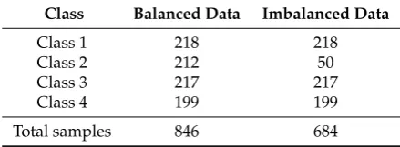
number of instances. However, class imbalance makes the learning task more complex. Figure1

shows the margin distribution of correctly classified training instances by bagging involving decision

tree as base learner on data setVehicle(Table1) in both balanced and imbalanced cases, using our

ensemble margin Equation (4). The margin values should be as high as possible for correctly classified

instances. From the margin plot, we can see that imbalanced data lead to more instances of obtaining high margin values and less instances with low margin values. In fact, the existence of one or more minority classes in a classification task results in majority classes obtaining more space. Thus causes a classifier bias to the classification of majority classes and an illusory optimized margin distribution for imbalance learning.

0 . 0 0 . 1 0 . 2 0 . 3 0 . 4 0 . 5 0 . 6 0 . 7 0 . 8 0 . 9 1 . 0

C

u

m

u

la

ti

v

e

d

is

tr

ib

u

ti

o

n

M a r g i n

[image:9.595.168.430.387.600.2]

I m b a l a n c e d d a t a B a l a n c e d d a t a

Figure 1.Margin distribution of correctly classified training instances by bagging with both balanced

and imbalanced versions of data setVehicleusing a new ensemble margin.

Table 1.Imbalanced and balanced versions of data setVehicle.

Class Balanced Data Imbalanced Data

Class 1 218 218

Class 2 212 50

Class 3 217 217

Class 4 199 199

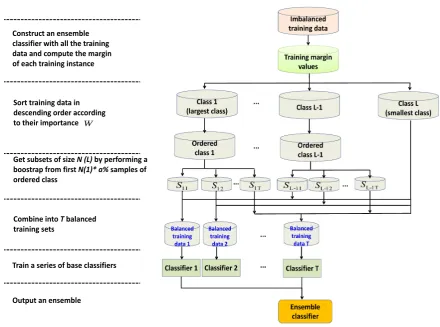
[image:9.595.187.407.676.757.2]

(10)

4. A Novel Bagging Method Based on Ensemble Margin

Compared to binary classification data imbalance problems, multi-class imbalance problems increase the data complexity and negatively affect the classification performance regardless of whether the data is imbalanced or not. Hence, multi-class imbalance problems cannot be simply solved by rebalancing the number of examples among classes in the pre-processing step. In this section, we propose a new algorithm to handle the class imbalance problem. Several methods proposed in the literature to address the problem of class imbalance as well as their strengths and weaknesses have been presented in the previous section. Ensemble classifiers have been shown to be more effective than data sampling techniques to enhance the classification performance of imbalanced data. Moreover, the combination of ensemble learning with sampling methods to tackle the class imbalance problem has led to several proposals with positive results in the literature.

In addition, as mentioned in the previous section, boosting based methods are sensitive to noise. On the contrary, bagging techniques are not only robust to noise but also easy to develop. Galar et al. pointed out that bagging ensembles would be powerful when dealing with class imbalance if they are

properly combined [5,63]. Consequently, we chose to found our new imbalance ensemble learning

method on bagging.

Enhancing the classification of class decision boundary instances is useful to improve the classification accuracy. Hence, for a balanced classification, focusing on the usage of the small margin instances of a global margin ordering should benefit the performance of an ensemble classifier. However, the same scheme is not suited to improve the model built from an imbalanced training set. Although most of the minority class instances have low margin values, selecting useful instances from a global margin sorting still has a risk to lose partial minority class samples, and even causes the classification performance to deteriorate. Hence, the most appropriate method for the improvement of imbalanced classification is to choose useful instances from each class independently.

4.1. Ensemble Margin Based Data Ordering

The informative instances such as class decision boundary samples and difficult class instances play an important role in classification particularly when it is imbalanced classification. These instances generally have low ensemble margins. To utilize the relationship between the importance of instances and their margins effectively in imbalance learning, we designed our class imbalance sampling algorithm based on margin ordering.

Let us consider a training set denoted asS = {X,Y} = {xi,yi}ni=1, wherexi is a vector with

feature values andyiis the value of the class label. The importance of a training instancexicould be

assessed by an importance evaluation function which relies on an ensemble margin’s definition and is

defined by Equation (5).The lower the margin value (in absolute value), the more informative the instance xi

is and the more important it is to consider for our imbalance sampling scheme.

W(xi) =1− |margin(xi)| (5)

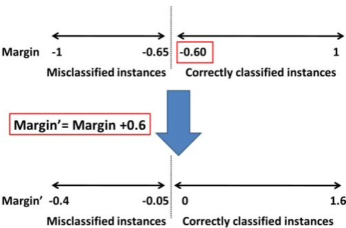
To solve the problem previously mentioned related to the margins (both supervised and unsupervised) based on a sum operation, a shift is performed before data importance calculation. The shifted margin values are achieved by subtracting the minimum margin value of the samples of the training set which are correctly classified from their original margin values. An example is used to

(11)

Misclassified instances Correctly classified instances

Margin -1 -0.65 -0.60 1

Misclassified instances Correctly classified instances

Margin’ -0.4 -0.05 0 1.6

[image:11.595.170.422.86.252.2]

Margin’= Margin +0.6

Figure 2.Shift procedure for sum operation based margin.

4.2. A Novel Bagging Method Based on Ensemble Margin

The proposed ensemble margin based imbalance learning method is inspired by

SMOTEBagging [8], a major oversampling method which has been defined in the previous

section. It combines under sampling, ensemble and margin concepts. Our method pays more

attention to low margin instances. It could overcome the shortcomings of bothSMOTEBagging[8] and

UnderBagging[38]. This method has lower computational complexity thanSMOTEBaggingand focuses

more on important instances for classification tasks thanUnderBagging.

The proposed method has three main steps:

1. Computing the ensemble margin values of the training samples via an ensemble classifier.

2. Constructing balanced training subsets by focusing more on small margin instances.

3. Training base classifiers on balanced training subsets and constructing a new ensemble with a

better capability for imbalance learning.

DenoteS = {X,Y}= {xi,yi}ni=1as training samples. The first step of our method involves a

robust ensemble classifier:baggingwhich is constructed using the whole training set. The margin value

of each training instance is then calculated. In the second phase, we aim to select the most significant

training samples for classification to form several new balanced training subsets. SupposeLis the

number of classes andNi the number of training instances of theithclass. We sort those classes in

descending order according to their number of instances. Therefore,NLis the training size of classL,

which is the smallest, andN1is the training size of class 1 which is the largest. The training instances

of each class, 16c6 L, are sorted in descending order according to the margin based importance

evaluation function (Equation (5)) previously introduced. For each classc, the higher the importance

valueW(xi)of an instancexi ∈c, the more important this instance is for classification decision. Then,

as inSMOTEBagging[8], a resampling rateais used to control the amount of instances which should

be chosen in each class to contract a balanced data set. All the instances of the smallest class are kept. The detailed steps of our method are shown in Algorithm 1.

The range ofais set from 10 to 100 first. For each classc6=L,Lrepresenting the smallest class,

NLinstances are bootstrapped from the firstN1·a% of the importance ordered samples of classcto

construct subsetSc1. All the subsets are balanced. When the amount of classc(26c6L−1)is under

N1·a%,NL instances are bootstrapped from the firstNcsamples of classc, which is the same as in

UnderBagging. Then theNLsmallest class samples are combined withSc1(c=1, ...,L−1)to construct

the first balanced data. In the next phase, the first base classifier is built using the obtained balanced

training set. Figure3presents the flowchart of our method with an ensemble sizeTand a range of

10–100% fora. The elements in the range ofacould construct an arithmetic progression denoted asA.

(12)

resampling ratesaranging from 10% to 100%, as inSMOTEBagging. However, whileSMOTEBagging

usesN1, the training size of the largest class 1, as a standard for carrying out oversampling (SMOTE) on

other relative minority classes, our method useNL, the training size of the smallest classL, as a standard

for performing an instance importance based undersampling on other relative majority classes.

Algorithm 1:A novel ensemble margin based bagging method (MBagging).

Training phase Inputs:

1. Training setS= (x1,y1),(x2,y2,),· · ·,(xn,yn);

2. Number of classesL;

3. Ni is the number of training instances of ith class NL 6 Ni 6 N1 (L = smallest class,

1=largest class);

4. Ensemble creation algorithmζ;

5. Number of classifiersT;

6. Range of resampling ratea.

7. E=∅: an ensemble

Iterative process:

1. Construct an ensemble classifier Hwith all then training data(xi,yi) ∈ S and compute the

margin of each training instancexi.

2. Obtain the weightW(xi)of each training instancexi.

3. Order separately the training instancesxi of each class, according to the instance importance

evaluation functionW(xi), in descending order.

4. Fort=1 toT do

(a) Keep all theNLinstances of the smallest classL

(b) Forc=1toL−1

i. IfNc>a%·N1

Get a subsetSct of sizeNL by performing a boostrap from firstN1·a% ordered

samples of the training setSc.

ii. else

Get a subsetSctof sizeNLby performing a boostrap fromNcsamples ofSc.

End

(c) Construct a new balanced data setStby combining theNLsmallest class training instances

withSct(c=1, ...,L−1).

(d) Train a classifierht=ζ(St).

(e) E←E∪ht.

(f) Change percentage a%.

End

Output:The ensembleE

Prediction phase Inputs:

1. The ensembleE={ht}T_t₌₁;

2. A new samplex∗.

Output:Class labely∗=argmax∑T

(13)

Combine into Tbalanced training sets

Sort training data in descending order according to their importance W

Get subsets of size N (L) by performing a boostrap from first N(1)* a% samples of ordered class

Construct an ensemble classifier with all the training data and compute the margin of each training instance

Train a series of base classifiers

[image:13.595.74.515.94.421.2]

Output an ensemble

Figure 3. Flowchart of margin based imbalanced ensemble classification (ensemble size T = 10,

range of resampling ratea10–100%).

5. Experimental Results

5.1. Data Sets

We applied our margin-based imbalance learning method on 18 UCI data sets including

17 multi-class and 1 binary data (Table2). Among these imbalanced data,Optdigit,PendigitandVehicle

are artificially imbalanced data. The 18 data sets are characterized by different sizes, class numbers and features. Furthermore, they differ in class imbalance ratio.

Table2summaries the properties of the selected data-sets, including the number of classes (CL),

the number of attributes (AT), the number of examples (EX) as well as the number of instances for each

class (Ci).

5.2. Experimental Setup

In all our experiments, Classification and Regression Trees (CART) are used as base classifiers for

training all the classification models. StandardBagging[71] is utilized to obtain the margin values of

training instances. All the ensembles are implemented with 100 trees. Each data set has been randomly divided into two parts: training set and test set. In order to avoid the case that all the minority class instances are in the training set (or test set), and there are no samples of the smallest class in the test set (or training set), the percentage of the instances used for training and testing is set to 1:1, i.e., 50% original data is obtained via adopting random sampling without replacement to form a training set, and all the unselected instances compose a test set. All the reported results are mean values of a

(14)

[image:14.595.89.510.110.321.2]

Table 2.Imbalanced data sets.

Data EX AT CL C1 C2 C3 C4 C5 C6 C7 C8 C9 C10

Car 1600 6 4 62 66 359 1113

Cleveland 297 13 5 13 35 35 54 160

Covtype.data 8000 54 7 33 139 241 278 481 2985 3843

Glass 214 10 6 9 13 17 29 70 76

Hayes-roth 160 4 3 31 64 65

Newthyroid 215 5 3 30 35 150

Optdigit 1642 64 10 20 40 180 187 191 196 197 197 210 224

Page-blocks 5472 10 5 28 87 115 329 4913

Penbased 1100 16 10 105 105 106 106 106 114 114 114 115 115

Pendigit 3239 16 10 20 20 362 379 394 396 397 408 426 437

Segment 2000 19 7 279 280 281 286 289 291 294

Statlog 5000 36 6 485 539 540 1061 1169 1206

Urbanlandcover 300 147 9 11 13 19 28 30 45 46 47 61

Vehicle 684 17 4 50 199 217 218

Wilt 4839 5 2 261 4578

Wine 178 13 3 48 59 71

Wine quality-red 1599 11 6 10 18 53 199 638 681 Wine quality-white 4898 11 7 5 20 163 175 880 1457 2198

5.3. Evaluation Methods

In the framework of imbalanced data-sets, standard metrics such as overall accuracy are not the most appropriate, since they do not distinguish between the classification rates of different classes,

which might lead to erroneous conclusions [45]. Therefore we adopt minimum accuracy per class,

F-measure,average accuracyanddiversityas performance measures in our experiments.

• Recall, also called per class accuracy, is the percentage of instances correctly classified in each

class. [10] strongly recommends using the dedicated performance measureRecallto evaluate

classification algorithms, especially when dealing with multi class imbalance problems. Letnii

andnijrepresent the true prediction of theith class and the false prediction of theith class into

jth class respectively. The per class accuracy for classican be defined as (6).

Recalli = _∑Lnii

j=1nij (6)

whereLstands for the number of classes

• Average accuracyis a performance metric that gives the same weight to each of the classes of the problem, independently of the number of examples it has. It can be calculated as the following equation:

AverageAccuracy = ∑iL=1Recalli

L (7)

• F-Measureis one of the most frequently used measurements to evaluate the performance of an algorithm for imbalance data classification. It is a family of metrics that attempts to measure the trade-offs between precision, which measures how often an instance that was predicted as positive is actually positive, and recalls by outputting a single value that reflects the goodness of

a classifier in the presence of rare classes [72].

F−measure= 2_L ∑Li=1Recalli∑Li=1Precisioni

∑L

i=1Recalli+∑iL=1Precisioni (8)

wherePrecisionican be computed by_∑Lnii

(15)

• KW Diversity[73] is a performance metric that gives the same weight to each of the classes of the problem, independently of the number of examples it has. It can be calculated as the following

equation [69]:

KW =− 1

NT2 ∑iN=1t(xi)(T−t(xi)) (9)

where diversity increases with KW variance,Tis the size of the ensemble of classifiers,t(xi)is the

number of classifiers that correctly recognize samplexi, andNrepresents the number of samples.

5.4. Imbalance Learning Performance Comparative Analysis

These experiments evaluate the classification performance of the proposed ensemble margin based imbalance learning algorithm, and its comparison to original bagging as well as state of the

art algorithms UnderBagging [38] and SMOTEBagging [8]. In addition, the performances of four

ensemble margin definitions in our margin based ensemble are compared. The best results are marked

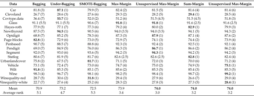
[image:15.595.88.514.320.481.2]

in bold. The values in parentheses of the Tables3–5represent the rank of the comparative methods.

Table 3.Average accuracy of standard bagging, UnderBagging, SMOTEBagging and margin-based bagging with four margins.

Data Bagging Under-Bagging SMOTE-Bagging Max-Margin Unsupervised Max-Margin Sum-Margin Unsupervised Max-Margin Car 79.7 (7) 91.9 (5) 84.0 (6) 93.4(1) 92.6(3) 92.7(2) 92.3 (4) Cleveland 28.1 (6) 29.2 (2.5) 28.9 (4) 29.2 (2.5) 28.0 (7) 29.5(1) 28.4 (5) Covtype.data 32.0 (7) 67.9 (3) 65.7 (6) 67.4 (5) 67.6 (4) 67.9 (3) 68.1(1) Glass 91.6 (6) 92.9 (5) 91.2 (7) 93.4(1) 93.4(1) 93.1 (3) 93.1 (3) Hayes-roth 77.3 (5) 76.8 (6) 76.1 (7) 79.2 (4) 79.9 (2.5) 82.9(1) 79.9 (2.5) Newthyroid 81.7 (7) 93.6 (5) 85.6 (6) 94.0 (3.5) 94.0 (3.5) 94.2 (2) 94.3(1)

Optdigit 69.4 (7) 87.5 (5) 80.4 (6) 89.7 (3) 90.5(1) 89.6 (4) 90.0 (2) Page-blocks 81.3 (7) 94.5 (2.5) 91.8 (6) 94.0 (5) 94.5 (2.5) 95.0(1) 94.3 (4) Penbased 90.6 (5) 88.4 (7) 88.7 (6) 92.5 (2.5) 92.5 (2.5) 92.6(1) 92.2 (4) Pendigit 62.4 (7) 88.0 (5) 76.9 (6) 90.2 (3) 90.3 (2) 90.4(1) 90.0 (4) Segment 91.4 (7) 92.5 (6) 93.3 (5) 93.8 (3) 93.9(1) 93.9(1) 93.8 (3) Statlog 78.7 (7) 81.5 (5) 81.4 (6) 82.3 (2.5) 82.3 (2.5) 82.8(1) 82.2 (4) Urbanlandcover 75.0 (2) 68.9 (7) 81.8(1) 72.2 (5) 73.2 (3) 71.5 (6) 72.4 (4) Vehicle 71.2 (7) 72.8 (6) 73.4 (5) 76.1 (4) 76.4 (2) 76.2 (3) 76.6(1) Wilt 87.2 (7) 94.7 (6) 95.0 (5) 95.5 (3) 95.5 (3) 95.6(1) 95.5 (3) Wine 98.2 (5) 96.9 (7) 98.0 (6) 98.3(4) 98.5 (3) 98.8 (2) 99.2(1) Wine quality-red 27.9 (7) 33.8 (2) 36.7(1) 33.3 (3) 31.6 (5) 30.6 (6) 33.1 (4) Wine quality-white 21.8 (7) 34.7 (4) 31.3 (6) 36.9 (3) 37.5 (2) 34.2 (5) 40.1(1)

Mean accuracy 69.2 77.0 75.6 78.4 78.5 78.4 78.6

[image:15.595.89.514.526.687.2]

Average rank 6.2 4.9 5.3 3.2 2.8 2.4 2.9

Table 4.F-measure of standard bagging, UnderBagging, SMOTEBagging and margin-based bagging with four margins.

Data Bagging Under-Bagging SMOTE-Bagging Max-Margin Unsupervised Max-Margin Sum-Margin Unsupervised Max-Margin Car 81.8 (3) 87.1(1) 79.9 (7) 82.4 (2) 81.5 (5) 81.6 (4) 81.4 (6) Cleveland 26.7 (7) 28.6 (3) 27.6 (6) 29.3 (2) 28.2 (5) 29.4(1) 28.5 (4) Covtype.data 36.4 (7) 53.7(1) 52.0 (2) 51.2 (6) 51.5 (4.5) 51.5 (4.5) 51.8 (3) Glass 91.1 (5.5) 91.1 (5.5) 90.6 (7) 91.8(1) 91.8(1) 91.6 (2.5) 91.6 (2.5) Hayes-roth 77.9 (5) 77.1 (7) 77.3 (6) 79.2 (4) 80.0 (2) 82.9(1) 79.9 (3) Newthyroid 87.5 (7) 94.5(1) 90.5 (6) 94.0 (3.5) 94.0 (3.5) 94.1 (5) 94.3 (2) Optdigit 68.8 (7) 85.2 (5) 78.3 (6) 87.3 (3) 87.9(1) 87.1 (4) 87.6 (2) Page-blocks 82.8(1) 72.9 (6) 73.0 (5) 72.9 (7) 74.1 (3) 74.4 (2) 73.9 (4) Penbased 90.7 (5) 88.5 (7) 88.8 (6) 92.3 (3) 92.4 (2) 92.5 (1) 92.1 (4) Pendigit 69.0 (7) 84.9 (5) 76.0 (6) 86.3 (3) 86.7(1) 86.6 (2) 86.2 (4) Segment 92.0 (7) 93.0 (6) 93.6 (5) 94.2 (3) 94.3(1) 94.2 (3) 94.2 (3) Statlog 80.6 (7) 81.9 (5) 81.7 (6) 82.6 (2.5) 82.6 (2.5) 82.8(1) 82.4 (4) Urbanlandcover 75.8 (2) 67.5 (7) 81.7(1) 71.1 (5) 72.0 (3) 70.0 (6) 71.2 (4) Vehicle 73.1 (5) 72.4 (7) 73.0 (6) 74.7 (4) 75.0 (2) 74.9 (3) 75.1(1) Wilt 91.8(1) 85.3 (5) 85.1 (7) 85.6 (2) 85.3 (5) 85.4 (3) 85.3 (5) Wine 98.3 (4) 96.7 (7) 98.1 (6) 98.2 (5) 98.4 (3) 98.7 (2) 99.2(1) Winequality-red 28.7 (5) 30.6 (2) 31.8(1) 29.4 (3) 27.9 (6) 26.6 (7) 29.0 (4) Winequality-white 22.7 (7) 27.6 (4) 25.2 (6) 28.3 (2) 27.8 (3) 27.3 (5) 28.4(1)

Mean 70.9 73.2 72.5 73.9 74.0 74.0 74.0

Average rank 5.1 4.7 5.3 3.4 3.0 3.2 3.2

5.4.1. Average Accuracy

Table3shows the average accuracy achieved by the proposed margin based extended bagging

algorithm, bagging, UnderBagging as well as SMOTEBagging on the 18 imbalanced data sets of

Table2. The experimental results in this table show that all the imbalance learning algorithms lead

(16)

[image:16.595.90.515.270.432.2]

ensemble classifiers such as margin based bagging and UnderBagging outperform oversampling based ensemble classifiers (SMOTEBagging). This result is consistent with the state-of-the-art work presented in the previous section, where we have explained that oversampling based methods have a risk of injecting additional noise into the training set. The ensemble model based on margin achieves the best performance, especially in addressing the imbalance problem of many-majority and less-minority classes, that often occurs in the real world. These results put a clear emphasis on the importance of preprocessing the training set prior to building a base classifier by focusing on the examples with low margin values and not treating them uniformly. Although there are not obvious differences between the performances of the four ensemble margin definitions, unsupervised margins perform slightly better than supervised margins. Max margins have very similar performances as sum margins.

Table 5. Minimum accuracy per class of standard bagging, UnderBagging, SMOTEBagging and

margin-based bagging with four margins.

Data Bagging Under-Bagging SMOTE-Bagging Max-Margin Unsupervised Max-Margin Sum-Margin Unsupervised Max-Margin Car 59.3 (7) 87.0 (4) 68.5 (6) 88.8 (1) 88.4 (2) 87.9 (3) 86.8 (5) Cleveland 0.0 (7) 0.0 (7) 0.0 (7) 7.4(1) 4.4 (3) 5.7(1) 3.4 (4) Covtype.data 0.0 (7) 41.2 (2) 46.4(1) 31.4 (4) 30.8 (6) 31.8 (3) 31.0(5) Glass 80.0 (3.5) 79.8 (7) 80.0 (3.5) 80.0 (3.5) 80.0 (3.5) 79.8 (7) 79.8 (7) Hayes-roth 47.6 (6) 53.5 (5) 41.1 (7) 68.1 (2) 69.2(1) 67.8 (3) 64.4 (4) Newthyroid 61.8 (7) 87.8(1) 72.4 (6) 85.0 (2.5) 85.0 (2.5) 84.2 (4.5) 84.2 (4.5)

Optdigit 0.0 (7) 71.4 (5) 61.3 (6) 78.1 (3) 79.6(1) 76.7 (4) 79.3 (2) Page-blocks 54.2 (7) 89.4 (3) 80.8 (6) 88.8 (5) 89.8 (2) 90.9(1) 88.9 (4) Penbased 79.4 (2.5) 76.9 (7) 76.9 (6) 78.8 (5) 79.4 (2.5) 79.7(1) 79.1 (4) Pendigit 0.0 (7) 77.8 (5) 33.3 (6) 72.8(1) 71.9 (2) 71.0 (3) 70.9 (4) Segment 79.3 (7) 79.3 (7) 79.7 (5) 82.5 (4) 83.3 (2) 83.4(1) 82.8 (3) Statlog 45.8 (7) 69.2(1) 67.7 (2) 59.1 (6) 59.2 (4.5) 62.8 (3) 59.2 (4.5) Urbanlandcover 37.3 (7) 40.9 (6) 66.7(1) 49.9 (3) 52.7 (2) 49.2 (4) 46.8 (5)

Vehicle 31.3 (7) 43.9 (2) 47.0(1) 40.8 (4) 39.1 (6) 41.7 (3) 39.3 (5) Wilt 74.0 (7) 92.8 (6) 94.4 (5) 95.4(1) 95.3 (2.5) 95.2 (4) 95.3 (2.5) Wine 94.7 (5) 94.1 (7) 94.1 (7) 96.7 (4) 97.3 (3) 97.7 (2) 98.2(1) Winequality-red 0.0 (7) 15.9 (4) 0 (7) 15.9 (4) 19.6(1) 14.2 (6) 16.9 (2) Winequality-white 0.0 (7) 9.7 (5) 0.0 (7) 13.0(1) 11.9 (3) 10.7 (4) 12.3 (2)

Mean accuracy 41.4 61.3 56.1 62.9 63.1 62.8 62.1

Average rank 6.4 4.7 5.0 3.1 2.8 3.2 3.8

5.4.2. F-Measure

For F-measure results presented in Table4, we can observe that, the best average of F-measure

is still achieved by margin based bagging. The achieved improvement of our algorithm is about

6%(data setHayer-roth) compared to UnderBagging and about10%(data setPendigit) with respect

to SMOTEBagging. Moreover, unsupervised margins slightly outperform supervised margins in

our method. In addition, for the binary dataWiltand multi-class dataPage-blockswhich is with the

imbalance ratio of up 175, all the improved bagging methods lose effectiveness. This means that imbalance classification algorithms still face great challenges in avoiding hurting the accuracy of majority class when increasing the accuracy of minority class in the case of very high imbalance rate.

5.4.3. Minimum Accuracy Per Class

Table5organized as the previous table, presents the results on minimum accuracy per class

obtained on the 18 imbalanced data sets of Table2by margin based bagging, traditional bagging,

UnderBagging as well as SMOTEBagging. This table shows that our extended bagging algorithm outperforms traditional bagging on the recognition of the most difficult class. With respect to

UnderBagging, the win frequency of our method is13/18and its improvement in per class classification

accuracy is up to15%(data setHayes-roth). When compared with SMOTEBagging, the margin based

method also obtains a win frequency of13/18and improves the minimum accuracy per class of up to

39%(data setPendigit). Unlike in the previous average accuracy margin analysis, unsupervised max

(17)

5.4.4. Statistical Analysis of Results

The above analysis of the behaviour and performance of classifiers was based on the groupings

formed by consideringaverage accuracy,F-measureandminimum accuracy per classon the datasets.

In order to extend the analysis provided above, a non-parametric statistical test [74,75] is conducted for

validating the effectiveness of margin based bagging method. The Friedman test is recognised as one of the best tests when multiple different datasets are used. Therefore, in our experiment, the Friedman

test [74] is leveraged to verify whether there is a significant difference among the mean ranks of

different alternatives when different algorithms provide varying performances on different data sets.

Tables3–5have provided a summary of mean ranks of comparative algorithms on all datasets. The null

hypothesisH0that we used was that the ranks ofaverage accuracy,F-measureandminimum accuracy

per classacross the three reference classifiers and the proposed method with four margin definitions

was the same. When the significant level is selected as 0.05, the null hypotheses H0in terms of all

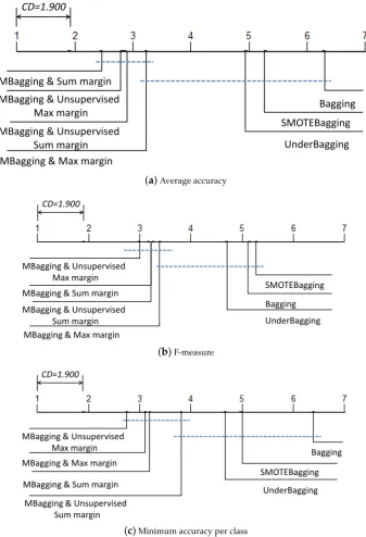
three metrics can be rejected. To verify whether our method performs better than other algorithms, we compute the critical difference (CD) chosen by the Bonferroni–Dunn post-hoc test.

Figure4presents the results of post-hoc tests onaverage accuracy,F-measureandminimum accuracy

per classfor comparative algorithms over all the datasets. If the difference between the mean ranks of two algorithms in terms of an evaluation metric is greater or equal to CD, then we can state that there is

a statistical difference between the two algorithms. As CD = 1.900, the Tables3and4performances of

margin based method are significantly better than that of bagging, UnderBagging and SMOTEBagging. Theminimum accuracy per classperformance of the proposed method with first three margin definitions is significantly better than that of bagging and other state-of-the-art methods. From the above analysis, we can state that the proposed method obtains a good tradeoff between the majority class and minority class performances when tested on multi-class imbalanced data sets. Furthermore, unsupervised max margin statistically outperforms other margins especially for the improvement of the classification of the smallest class instances.

5.4.5. Diversity

Ensemble diversity is a property of an ensemble with respect to a set of data. It has been recognized as an important characteristic in classifier combination. Ensemble methods can effectively make use of diversity to reduce the variance-error without increasing the bias-error. In other words, ensemble learning is very effective, mainly due to the phenomenon that base classifiers have different “biases”.

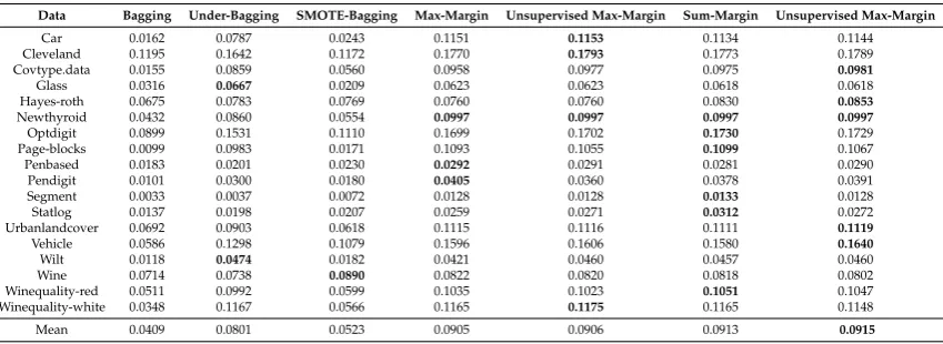
Table 6shows the ensemble diversity of the proposed method, original bagging, UnderBagging

and SMOTEBagging. This table shows that, with respective to the traditional data sampling based methods, the margin guiding ensemble is not only more accurate for the classification of multi-class imbalanced data, but also leads to more ensemble diversity. Hence, the ability of the novel algorithm is demonstrated again.

5.4.6. Time Complexity and Space Complexity

Over sampling techniques such asSMOTEBaggingare computationally more expensive than

traditional bagging and under sampling based methods as a result of having a larger training set.

The time complexity of bagging isO(NF(X)), whereNandF(X)respectively stands for the number

of samples in a datasetXand the training complexity of an algorithm given a datasetX[76]. The time

complexity ofUnderBaggingisO(RF(Q)), whereRis the number of samples in a datasetQwhich

is a subset taken from the datasetX[76]. The time complexity of our approach arises mainly from

two sources: the computing of the training instances margins using bagging and the building of the following under sampling combined bagging model. Therefore, the overall time complexity of

our proposal is the sum of that of bagging andUnderBagging,O(NF(X) +RF(Q)), i.e., the proposed

(18)

our method is slightly more computationally consuming, the time complexity of our method will decrease with the increase in imbalance ratio, because it is based on the under sampling technique.

CD=1.900

MBagging & Sum margin

Bagging SMOTEBagging MBagging & Unsupervised

Max margin

MB i & U i d gg g

UnderBagging MBagging & Max margin

MBagging & Unsupervised Sum margin gg g g

(a)Average accuracy

CD=1.900

Bagging SMOTEBagging

MBagging & Unsupervised Max margin MBagging & Sum margin MBagging & Unsupervised

Sum margin

(b)F-measure

CD=1.900

Bagging SMOTEBagging

MBagging & Unsupervised Max margin

MBagging & Sum margin MBagging & Unsupervised

Sum margin

[image:18.595.126.464.131.626.2]

(c)Minimum accuracy per class

Figure 4. Bonferroni-Dunn (95% confidence level) for the comparative methods on all data sets (ensemble size = 100).

The space complexity of bagging andUnderBaggingare allO(ND)whereDis the number of

(19)

[image:19.595.88.513.122.277.2]

Table 6. Ensemble diversity of standard bagging, UnderBagging, SMOTEBagging and margin-based bagging with four margins.

Data Bagging Under-Bagging SMOTE-Bagging Max-Margin Unsupervised Max-Margin Sum-Margin Unsupervised Max-Margin

Car 0.0162 0.0787 0.0243 0.1151 0.1153 0.1134 0.1144

Cleveland 0.1195 0.1642 0.1172 0.1770 0.1793 0.1773 0.1789

Covtype.data 0.0155 0.0859 0.0560 0.0958 0.0977 0.0975 0.0981

Glass 0.0316 0.0667 0.0209 0.0623 0.0623 0.0618 0.0618

Hayes-roth 0.0675 0.0783 0.0769 0.0760 0.0760 0.0830 0.0853

Newthyroid 0.0432 0.0860 0.0554 0.0997 0.0997 0.0997 0.0997

Optdigit 0.0899 0.1531 0.1110 0.1699 0.1702 0.1730 0.1729

Page-blocks 0.0099 0.0983 0.0171 0.1093 0.1055 0.1099 0.1067

Penbased 0.0183 0.0201 0.0230 0.0292 0.0291 0.0281 0.0290

Pendigit 0.0101 0.0300 0.0180 0.0405 0.0360 0.0378 0.0391

Segment 0.0033 0.0037 0.0072 0.0128 0.0128 0.0133 0.0128

Statlog 0.0137 0.0198 0.0207 0.0259 0.0271 0.0312 0.0272

Urbanlandcover 0.0692 0.0903 0.0618 0.1115 0.1116 0.1111 0.1119

Vehicle 0.0586 0.1298 0.1079 0.1596 0.1606 0.1580 0.1640

Wilt 0.0118 0.0474 0.0182 0.0421 0.0460 0.0457 0.0460

Wine 0.0714 0.0738 0.0890 0.0822 0.0820 0.0818 0.0802

Winequality-red 0.0511 0.0992 0.0599 0.1035 0.1023 0.1051 0.1047

Winequality-white 0.0348 0.1167 0.0566 0.1165 0.1175 0.1165 0.1148

Mean 0.0409 0.0801 0.0523 0.0905 0.0906 0.0913 0.0915

5.5. Influence of Model Parameters on Classification Performance

5.5.1. Influence of the Ensemble Size

The results presented so far were about the ”final” bagging made of 100 trees. In order to study the

influence of ensemble size on bagging construction, we present in Figure5the evaluation of theaverage

accuracy,F-measureandminimum accuracy per class, which are average values through all the datasets, with respect to ensemble size throughout the bagging induction processes, i.e., from 1 up to 150 trees for all the bagging methods. We can observe that a larger ensemble size is beneficial to the classification improvement of the multi-class imbalance data. However, it could lead to increased computational complexity. In particular applications, the balance between the computational complexity and the performance should be considered. One of the main objectives with the design of our algorithm is to obtain a performance improvement while ensemble less trees, faster and in a more straightforward way than with traditional bagging, UnderBagging and SMOTEBagging. Although, the curves of

Figure5have similar trends for those imbalance learning algorithms. The margin based bagging

curves have a faster increase from 1 to about 30 trees. This has a practical interest since it means that designing a stopping criterion based on performance will be possible for the margin based bagging induction to achieve good performance with low time complexity. This stopping criterion has not yet been included in the process of our margin based algorithm, but it is an important mechanism to design in future work.

5.5.2. Influence of the Resampling Rate

This section aims to study the influence of the resampling ratea on margin-based bagging

performance in imbalanced classification. We first employ the following example to illustrate our

experimental design. The maximum value of the resampling rateashould be equal to or less than 100.

When the size ofA, the associated set ofavalues, is set to 5, the elements ofAare{20, 40, 60, 80, 100},

i.e., the range of a is 20–100. When A = {100}, our margin based method becomes similar to

UnderBagging.

In this experiment, the sizeT of the bagging ensemble is set to 100 and the tested number of

elements inAis set from 1 to 40. Figures6–8exhibits the optimal range ofawhich respectively lead

to the bestaverage accuracy, F-measureandminimum accuracy per classfor each of the four margin

definitions, on all the data sets. Almost all the classification results are improved compared with those

of Tables3–5. The best increase in average accuracy is about 1.5% for most data. The best increase

in minimum accuracy per class is about10%for datasetsCovtype,StatlogandVehicle. Hence, it is

(20)

0 1 5 3 0 4 5 6 0 7 5 9 0 1 0 5 1 2 0 1 3 5 1 5 0 5 5

6 0 6 5 7 0 7 5 8 0

B a g g i n g U n d e r B a g g i n g S m o t e B a g g i n g M a x - m a r g i n

U n s u p e r v i s e d m a x - m a r g i n S u m - m a r g i n

U n s u p e r v i s e d s u m - m a r g i n

A

(%

)

N u m b e r o f c l a s s i f i e r s

(a)Average accuracy

0 1 5 3 0 4 5 6 0 7 5 9 0 1 0 5 1 2 0 1 3 5 1 5 0

5 0 5 5 6 0 6 5 7 0 7 5

F

-m

e

a

s

u

re

(%

)

(b)F-measure

0 1 5 3 0 4 5 6 0 7 5 9 0 1 0 5 1 2 0 1 3 5 1 5 0

3 0 3 5 4 0 4 5 5 0 5 5 6 0 6 5

M

in

im

u

m

a

c

u

ra

c

y

p

e

r

c

la

s

(%

)

[image:20.595.84.510.89.479.2]

(c)Minimum accuracy per class

Figure 5.Evolution of the average accuracy, F-measure and minimum accuracy per class according to the ensemble size.

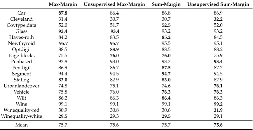
Tables 7–9 respectively present the average accuracy, F-measure and minimum accuracy

per class, achieved by our margin-based bagging algorithm using respectively max-margin, unsupervised max-margin, sum-margin and unsupervised sum-margin with optimal resampling ranges, on all the data sets. The exhibited results correspond to the classification results presented in

Figures6–8. From these tables, we can see that sum margins obtain slightly better results compared

(21)

[image:21.595.78.516.122.348.2]

Table 7. Average accuracy of margin-based bagging involving four margins with optimal resampling range.

Max-Margin Unsupervised Max-Margin Sum-Margin Unsupervised Sum-Margin

Car 94.1 93.7 93.8 93.9

Cleveland 30.6 28.0 31.0 29.4

Covtype.data 67.8 68.1 67.9 68.1

Glass 94.3 94.3 94.3 94.3

Hayes-roth 84.3 83.8 84.3 83.4

Newthyroid 95.8 95.7 95.9 95.1

Optdigit 90.5 90.9 90.9 90.9