CFD study of fluid flow changes with erosion

CFD study of fluid flow changes with erosion

Alejandro L´opeza,∗, Matthew T. Sticklanda, William M. Dempstera

a_{Department of Mechanical and Aerospace Engineering, Strathclyde University, Glasgow,}

United Kingdom

Abstract

For the first time, a three dimensional mesh deformation algorithm is used to

assess fluid flow changes with erosion. The validation case chosen is the Jet

Im-pingement Test, which was thoroughly analysed in previous works by Hattori

et al [1], Gnanavelu et al. in [2, 3], Lopez et al in [4] and Mackenzie et al in

[5]. Nguyen et al showed the formation of a new stagnation area when the wear

scar is deep enough by performing a three-dimensional scan of the wear scar

after 30 minutes of jet impingement test in [6] . However, in the work developed

here, this stagnation area was obtained solely by computational means. The

procedure consisted of applying an erosion model in order to obtain a deformed

geometry, which, due to the changes in the flow pattern lead to the formation

of a new stagnation area. The results as well as the wear scar were compared

to the results by Nguyen et al [6] showing the same trend. OpenFOAMR was

the software chosen for the implementation of the deforming mesh algorithm

as well as remeshing of the computational domain after deformation.

Differ-ent techniques for mesh deformation and approaches to erosion modeling are

discussed and a new methodology for erosion calculation including mesh

defor-mation is developed. This new approach is independent of the erosion modeling

approach, being applicable to both Eulerian and Lagrangian based equations

for erosion calculation. Its different applications such as performance decay in

machinery subjected to erosion as well as modeling of natural erosion processes

∗_{Corresponding author}

are discussed here.

Keywords: Erosion, OpenFOAM, multiphase, discrete phase model, Fluid

Surface Interaction, Mesh Deformation

1. Introduction

Erosion is responsible, amongst others, for destroying a wide variety of

equip-ment and causing vast losses in all kinds of industries. For over 50 years,

en-gineers have been trying to understand the process and, as a result, a large

number of scientific papers have been published on this subject. Most of these

authors have captured their very own and specific ideas about the way erosion

mechanisms work as well as the equations to predict wear in a number of

differ-ent geometries. Meng and Ludema [7] carried out a broad literature review of

more than 5000 papers dating from 1957 to 1992. In their article they identified

28 separate erosion models out of the almost 2000 existing empirical models,

a fact which exemplifies the poor agreement between authors on this subject.

One of the few theories on which there seems to be some kind of agreement

describes two mechanisms acting together to produce the wear scar: cutting

and deformation wear. When particles hit the surface and they tear material

away with them in a cutting action, it is called cutting wear. This mechanism is

the predominant one for ductile materials and particles impinging at low angles

of attack with respect to the surface being eroded. Alternatively, several

par-ticles might impact on the same place transferring some of their kinetic energy

to the surface in the form of hardening work [8]. According to this theory, in

a given collision with the target material, as soon as the particle contacts the

surface, stress concentrations appear as a result of the elastic deformation that

takes place. If these stresses are not over the elastic limit of the target material,

and also leaving aside fatigue damage effects, they should cause no

deforma-tion. However, if the elastic limit is reached, plastic deformation will occur at

the location of the maximum stress. The repeated impacts then create a

collisions. This deformation causes hardening and increases the elastic limit in

that region turning the material harder and more brittle until it reaches a point

where it can no longer be plastically deformed. Eventually, upon further load,

pieces of the material’s surface separate from the target and are carried away

by the fluid. This hypothesis was studied by Davies in [9], and Van Riemsdijk

and Bitter in [10] and then adopted by several authors [11, 8, 12, 13, 14]. This

mechanism is called deformation wear and it predominates for high angles of

impingement and in brittle materials. Erosion by solid particle impingement,

however, is just one of the types of erosion investigated and to which the

defor-mation algorithm can be coupled. Another recurrent erosion type, especially in

natural processes, is described in [15], [16], [17] and [18]. This type of erosion

is a consequence of erodible bodies moving in viscous fluids which results in a

purely fluid-mechanical erosion driven by the fluid’s shear stress acting on the

eroding boundaries. In processes such as erosion-corrosion, pure fluid erosion

could play a role in increasing material losses once the outer layers of the target

are corroded, thus increasing the total mass losses and possibly accounting for

synergistic effects. Synergy has been defined as the additional wear rate

experi-enced by the target material when both erosion and corrosion occur at the same

time. The synergistic effect can be calculated by substracting the pure erosion

and corrosion rates from the combined erosion-corrosion wear rate [19]. This

can be represented in the form of equation 1. Where T is the total wear rate,

E and C are the pure erosion and corrosion wear rates respectively and S is the

synergistic effect.

S=T−(E+C) (1)

By means of a combination of both types of erosion (purely fluid and solid

particle erosion), a new approach for calculating erosion-corrosion scars could be

derived, including the corrosion rate of the material in addition to fluid erosion

as well as solid particle erosion. In order to acquire a better understanding of

This algorithm enables knowing how erosion changes the shape of the domain,

how the fluid flow changes with it and its effect on the erosive process. In

addition, coupling the algorithm with different erosion approaches could provide

new insights into other erosive processes.

2. Erosion calculation in an Eulerian-Lagrangian frame

In this approach, previously discussed in [4], the Eulerian equations are

solved for the fluid phase and Newton’s equations (2, 3) are integrated for the

particles constituting the Lagrangian phase.

mp

dup

dt =Fp (2)

dxp

dt =up (3)

Where mp andup are the mass and velocity of the particle,Fp represents

the forces acting on the particle andxp the position of the particle.

Impingement information, such as impact velocity and impact angle, is

gath-ered by a function as particles hit the walls of the geometry. This information is

introduced in an erosion model implemented in OpenFOAM in order to obtain

an erosion field. The erosion formula chosen for comparison is the one developed

by Tabakoff et al in [20].

3. Eulerian phase steady-state

An equivalent domain to the one used by Nguyen et al in [6] was set up. The

mesh was composed of 2057316 elements, mainly hexahedral and the boundary

types used are shown in figure 1. Convergence criteria were satisfied for the

fluid phase when the residuals fell below 10−4 with second order schemes. The

results of the steady state simulation for velocity and pressure are shown in

Figure 2: Velocity contours of the uneroded geometry (m_s)

Different turbulence models were assessed for the jet impingement. The

first one was the k− model [21], which has repeatedly been used to predict

erosion in the jet impingement test as well as other configurations [6, 22, 2, 3]

and the second one was thek−ωSST model [23]. The k−model is a

semi-empirical model composed of two equations offering reasonable accuracy at an

acceptable computational cost. These reasons make it very popular in industrial

applications and over a wide range of flow regimes [24]. On the other hand, the

Shear Stress Transport (SST)k−ω brings togetherk-ω’s robust and accurate

formulation near the walls withk−’s free-stream independence in the far field

[24]. In a recent publication, the validity and accuracy of some of the most

widely used turbulence models (includingk− and k−ωSST) was assessed

by Mackenzie et al in [5] against Particle Image Velocimetry of the fluid phase,

concluding from the profiles of the velocities close to the impingement area that

the most widely used one, which is the k− model, is able to capture the

general trend of the axial and radial velocities at a reasonable computational

cost. With the known limitations of two-equation turbulence models, thek−

model seems like a reasonable approach, given that it is the general trend of the

velocity vectors, what will define the form that the wear scar takes. Additionally,

thek−model was also used by Nguyen et al after validating its accuracy in

[6] and, given that the aim in this work is to reproduce the results obtained

experimentally in that previous study, the same turbulence model is used here.

4. Discrete phase modeling

Once the steady-state values for the main flow field variables were obtained,

these were set as the initial conditions for the transient simulations. Particle

tracking is carried out by numerically integrating the sum of the forces acting

on the particles in order to obtain velocities and positions. The force balance

according to equation 2 for the case considered is shown in equation 4:

Fp=mp

dup

No forces other than the drag force were considered since their values

rela-tive to the drag force were negligible. Several additional simulations were run

incorporating other forces such as added mass, gravity etc with no significant

differences in the results for the averages of the velocity and impact angle on the

target. The drag force (FD) on spherical particles takes the form of equation

5 and the drag coefficient is obtained from equation 6, which is composed of

three parts corresponding from top to bottom of the equation to the Stokes’

Law region, the Transition region and the Newton’s Law region respectively.

FD=mp

18µ ρpd2p

CDRep

24 (u−up) (5)

CD=          24

Rep :Rep<1

24

Rep(1 + 0.15Re

0.687

p ) : 1≤Rep≤1000

0.44 :Rep>1000

(6)

Some of the features corresponding to the transient simulation are shown in

Table 1:

Variable Units Value

Time-step s 1∗10−05

Number of time-steps - 1∗106

Particle diameter distribution - Rosin-Rammler [25]

Particle diameter maximum Value m 180∗10−6

Particle diameter minimum Value m 125∗10−6

Coupling between phases - One-way

Forces - Drag

Drag coefficient - nonSphereDrag

Phi (Sphericity coefficient) - 0.58

Particle density Kg_m3 2400

Table 1: Transient simulation features

not spherical, a sphericity coefficient phi was set for the non-spherical drag

equation.

5. Erosion calculation and mesh deformation in OpenFOAM

In the following section, the procedure followed to deform the mesh according

to the erosion field is explained in detail. First, the application used to compute

the erosion field is described. Thereafter, the procedure consists of a series of

operations with the erosion field until the desired output is reached. It is after

this transformations that the mesh boundary will be deformed by means of an

extension of an application calleddeformedGeom, which allows moving the mesh

boundary according to a field of vectors stored at each time step.

5.1. Erosion modelling in OpenFOAM

In order to calculate erosion in OpenFOAM, one of the available Lagrangian

libraries was extended. One of the classes OpenFOAM provides the users with

is theCloudFunctionObjects. This is a templated library that adds additional

capabilities to the Lagrangian. The main template discussed here is called

particleErosion. This set of files create the particle erosion field on the

user-specified patches. The result is a field of scalars, which, at each face, will be the

sum of the volume eroded by all the particle hits. Impingement information,

such as impact speed and impact angle, is gathered as particles hit the walls of

the geometry. These are then introduced in the desired formulae, when different

erosion models, as in this case, are implemented inside the library. Functions

within the library give access to the particle variables at the moment of impact

with the target so that these values can be introduced in the erosion formula in

order to compute the erosion field.

One of the common issues that was addressed relates to the number of

im-pacts needed to obtain a good average for the erosion field. In order to calculate

how many impacts on the target are needed for an accurate representation of

Once the steady state in the transient simulation is reached, i.e., the number

of particles within the control volume doesn’t change or fluctuates around a

number, the parameters that allow calculation of the size of the sample needed

are obtained. Three new fields are also computed which give some insight into

how the averages are evolving during the simulations. These can be written to

memory at any time step. For the particular case of a discretised plane, as in

the boundary being impinged by particles, the total area (surface of the target)

is divided into a set of faces. This means that, as the simulation progresses, a

mean and a standard deviation can be calculated for each of the faces of the

boundary. By running a transient simulation, a time for which the mean values

and the standard deviation stop changing can be found. Once that simulation

has been studied and the mean and standard deviation values satisfying the

criteria are met, two meaningful values for each of the faces (the mean and the

standard deviation) are produced. With these two values and the formula used

for calculating the size of a sample, the minimum number of particles necessary

for a good average can be obtained. In order to calculate the size to obtain a

good average of the erosion field first, the level of confidence has to be specified.

In this case, if this level is set to be 99%, looking on the table of the Normal

Distribution it can be inferred thatzα

2 = 2.576. In addition to that, the error

needs also be specified. For this variable, a 5 per cent of the mean velocity at

each cell is chosen. The procedure is illustrated equations 7 and 8, of which

the latter is used for calculating the sample size for each of the faces of the

boundary.

δ=z

α

2σ √

n (7)

n= (z

α

2σ

δ )

2 ₍₈₎

Where δ is the maximum error of the estimate or the half-width of the

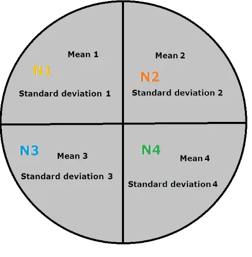
confidence interval, n is the size of the sample andσis the standard deviation

Figure 4: Representation of a circular domain divided in four faces, where N1, N2, N3 and

With the statistical analysis outlined in this section the minimum number

of impacts needed to obtain both velocity and impact angle averages with a

certain degree of confidence can be calculated. In order to do this, 10 seconds of

erosion were simulated for the case studied by Nguyen et al [6]. Initially, a visual

inspection of the results for different times, showed that the wear scar variations

after the first second of simulation were negligible, as shown in figure 5, where

the wear scar was obtained using the formula developed by Tabakoff et al [20].

These figures show how the contours only increase their values without changing

the shape of the scar from the first second of simulation. The formula used in

the calculations is shown in equation 9, whereis equal to the erosion per unit

mass of particles,β1is the relative angle between the particle trajectory and the

surface,β0 the angle of maximum erosion, V1 the velocity of the particle and

RT the tangential restitution ratio. Values for the empirical constantsK1,K12

andK3were calculated for aluminium in [20] and their values are 1.56988e−6,

0.3193 and 2.0e−12 respectively.

=K1f(β1)V12cos2β1(1−RT2) +f(VIN)

RT = 1−0.0016V1sinβ1

f(β1) = [1−CKK12sin(90_β0)β1]2

CK =







1 β1≤3β0

0 β1>3β0

(9)

Since one of the aims is to optimise the computational time invested in

run-ning the simulation, the results between time 0 s and 1s were analysed every

0.1 s of simulation. In addition to this, with the aid of the statistical fields

developed, the minimum number of impacts required per face were calculated.

The results after 10 seconds of simulations were used in order to calculate this

minimum number of impacts with a confidence level of 99%. The number of

particles released after 10 seconds was 1 million. Additionally, an application

was compiled in order to sum up the minimum number of impacts required at

each face for the impact angle and impact velocity averages. Of the two numbers

Figure 5: Contours of erosion per unit mass of impacting particles at 4 different simulation

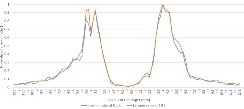
Figure 6: Contours of erosion per unit mass of impacting particles at 0.5 and 10 seconds of

simulation

value obtained for the simulation was 48677 impacts (or 0.48677 s). However,

this value only accounts for the time at which the particles are released. Thus,

the average time that a particle spends inside the domain was added to the

0.48677 seconds. The calculation of the average time a particle spends in the

domain was obtained from the log of OpenFOAM’s particle variables and

esti-mated to be 0.02 seconds for this simulation. It was after this simulation time

that the number of particles within the domain fluctuated around a constant

value. Therefore, the total time was rounded up to 0.5 seconds of simulation.

A qualitative comparison between the erosion contours at time 0.5 seconds and

10 seconds is shown in figure 6. Figure 7 shows a comparison of the normalised

erosion ratio between the same two time-steps plotted along the radius of the

target. The average difference between lines is 1.19%, which validates the

sta-tistical accuracy of the erosion contours at 0.5 s.

However, this process can be made in two different ways: an escape condition

can be set up at the target’s boundary (as done by Gnanavelu et al in [2, 3]) in

which the particles are eliminated from the domain as soon as they reach any of

the faces of the boundaries, or a rebound model may be chosen (or implemented)

in which rebound coefficients are defined for the particles. If the latter is used,

Figure 7: Comparison of the normalised erosion ratio over the radius of the probe (mm)

8 and 9 since the first impacts have the highest kinetic energy and a big part of

it is lost thereafter.

Differences are also spotted in the mean angle of impingement and also, the

number of impacts is around 1.5∗105_{times higher, as can be observed in images}

10, 11, 12 and 13.

5.2. Influence of the rebound model

The computational erosion obtained by Nguyen et al in [6] incorporated a

different erosion model than the default one in OpenFOAM. The model used

was developed by Forder et al in [27]. Forder’s model was implemented in

Open-FOAM and a 10 s simulation was obtained for each model. The erosion contours

obtained after 10 seconds are shown in figure 14. As can be observed, the wear

scars obtained with both models are practically identical. The only difference

between both scars relates to the magnitude of the erosion. This indicates that

a simple model, which would also be less computationally expensive, would be

sufficient to calculate erosion with enough accuracy for this configuration.

For validation of the mesh deformation algorithm a total of 10 seconds of

transient simulation is set up and the fields are monitored every 0.2 seconds.

Figure 8: Face-wise impact velocity average (m_s) after 10 seconds with an escape condition at the target’s boundary

Figure 10: Face-wise impact angle average (degrees) after 10 seconds with an escape condition

at the target’s boundary

Figure 12: Face-wise impact number after 10 seconds with an escape condition at the target’s

boundary

Figure 13: Face-wise impact number after 10 seconds with Forder’s [27] rebound model at the

Figure 14: Contours of erosion per unit mass of impacting particles for the same erosion model

[20] and different rebound models. Forder et al [27] (left) and OpenFOAM’s default rebound

model (right)

impacts and the velocity and angle averages will be taken from the case with

the rebound model developed by Forder et al [27] that was also implemented in

OpenFOAM. This rebound model was also the same one used by Nguyen et al

in [6].

5.3. Mesh deformation according to erosion

Once the erosion field has been calculated, the mesh deformation can be

accomplished through modification of the surface and by moving the boundary

points. Once steady state erosion is reached, the wear scar varies in magnitude

but its location and shape remain unchanged. Hence, the erosion field can be

subjected to an amplification which would be the equivalent of advancing the

simulation in time. This seems reasonable provided that, after a certain number

of impacts which can be calculated through sample size determination, the shape

of the scar does not vary significantly until the flow does. This so called steady

state erosion has been observed before by Huttunen-Saarivirta et al and Head

et al among others in [28, 29]. The erosion field calculated contains a value at

each of the boundary faces and it has a value of zero for all the internal cells.

A field that contains all the surface area vectors is then created. A surface area

the face and its magnitude is the area of the face. At the boundaries, the face

area vectors will point outside of the domain and these will give the direction

for the point displacement. As the magnitude of the displacement of the mesh

points will be equal to the magnitude of the erosion, unit normal vectors are

required. By dividing the face area vectors by their magnitude, the unit face

area normal vectors are obtained as defined in equation 10.

ˆ

u= u

kuk (10)

A field of vectors orthogonal to each of the boundary faces is stored to

memory. This field will be used to multiply it by the erosion field of scalars.

The final step before being able to move the mesh points is to interpolate the

field values contained at each face of the boundaries to each point of those

faces using an inverse distance weighting interpolation algorithm. The same

methodology for mesh deformation was applied in combination with dynamic

meshing. In doing this, a new solver for erosion calculation was created in

which the mesh is updated according to the user’s instructions and after mesh

deformation, the flow field is recalculated, thus, avoiding extra computational

time.

5.4. Validation of the 3-dimensional wear scar

An equivalent case to that one of Nguyen et al [6] was set up for validation.

Steady state results were computed first and after that, an Euler-Lagrange

sim-ulation was run in OpenFOAM in order to calculate erosion induced by solid

particle impingement. The parameters of the simulation were set to be the same

as the ones used by Nguyen et al in [6]. The formula used for prediction of the

erosion contours was developed by Tabakoff et al in [20] and implemented in

OpenFOAM. This model was run alongside other models such as the ones

devel-oped by Menguturk et in [30] (also discussed in [31] and [32]) and Nandakumar

et al [33] producing for all of them very similar erosion profiles and only differing

Figure 15: Wear scar profile depth comparison (µm) along the radius (mm) for different

scaling factors

Once the erosion ratios were calculated, the scar was scaled so that the

maxi-mum depth was 542µmand the steady state was calculated again. The scaling

factor which corresponds to 542µmof depth was 0.0349 for the erosion contours

obtained with the proposed formula. Additionally, different scaling factors were

applied in order to analyse the evolution of the fluid flow during the steady state

erosion. A radial average of the wear scars was obtained for each scaling factor

and the different profiles are shown in figure 15

A quantitative comparison between the wear scar profile obtained with

sim-ulations and the ones measured by Nguyen et al is shown in Figure 16. It was

also found that, as the scar progresses, the new stagnation point is captured,

validating the deformation algorithm. As opposed to the work developed by

Nguyen et al in [6], where the wear scar is 3D scanned and introduced into the

CFD software again, the results here were obtained entirely computationally

after 10 s of simulation . The initial contours of velocity and pressure are shown

in figures 2 and 3 respectively while the same are shown in figures 17 and 18

respectively for the deformed geometry after being eroded for a value of the

scaling factor of 0.00349.

Figure 16: Wear scar profile comparison with the experimental scars measured by Nguyen et

Figure 17: Velocity contours of the eroded geometry (m_s) for a scaling factor of 0.00349

analysed in figure 16.

Figure 20 shows the different surfaces obtained after the mesh deformation

for the same scaling factors.

Figure 21 shows the pressure contours at the deformed surfaces for all the

scaling factors with different scales for the pressure. This figure seems to

in-dicate that the stagnation point appears even before an equivalent depth to

the experiment of Nguyen et al [6]. In the computational calculation, the first

appearance of the stagnation point was detected for a scar depth 1.766 times

smaller than that the one reported by Nguyen et al in [6].

It is worth noting that the values of the pressure around the stagnation area

increase as the wear scar progresses while the location of the stagnation point

doesn’t change its relative location. However, the maximum velocity generated

by the new scars significantly changes its value at around the same depth

anal-ysed by Nguyen et al in [6], which corresponds to a scaling factor of 0.00349.

After that point, it fluctuates between different values, not increasing any

fur-ther. Therefore, it is predicted that the fluid flow changes would be significant

enough to affect particle trajectories once the wear scar is around 540 µm in

depth which could be confirmed by calculating erosion on the updated surfaces

to see if the shape of the erosion scar changes between the different depths.

These results confirm the validity of the approach for the wear scar obtained by

Nguyen et al in [6] after 30 minutes of erosion.

5.5. Time-scaling

The proposed methodology introduces three different time-scales. These

scales are optimised in order to calculate the deformed state of the geometry

once eroded in the minimum amount of time possible.

5.5.1. Lagrangian particles

The Lagrangian time-scale is related to the time-step set in the solver in

order to calculate particle trajectories accurately. In this type of simulations the

Figure 20: Surfaces obtained for all the scaling factors. From top to bottom and left to right:

0.001976, 0.0027, 0.00349, 0.00428

are calculated accurately. The lower the Courant-number, the more accurately

these will be calculated. In theory, the Courant number should be kept below

a value of 1. In the simulations shown in this work, the Courant number was

kept between 0.2 and 0.9. The Lagrangian time-step used in the simulations for

validation was 1e−5s.

5.5.2. Erosion and mesh deformation

The time-scale related to both erosion rate and mesh deformation, will be

dependent upon the number of impacts necessary in order to calculate the wear

scar with the chosen level of confidence. The mesh deformation time-scale will

have the same value, as the algorithm will be applied when the wear scar is

accurate enough. In this case, as it was outlined in this section, this value

should be equal to 0.5 seconds.

5.5.3. Fluid flow

Finally, the fluid-flow time-step should have the same value as the erosion

Figure 21: Pressure contours (P a) at the surfaces for all the scaling factors. From top to

deformed, the fluid flow steady state has to be recalculated in order to compute

the modified particle trajectories. Regarding the number of iterations of fluid

flow in order to achieve a new steady state, this will depend on the complexity

of the geometry on which erosion is calculated.

6. Erosion calculation with a dynamic mesh solver

In section 5.4, the mesh was refined after deformation through creation of

layers between the boundary and the cells next to it. A different technique was

implemented in order to avoid having an increasing size of the cells adjacent to

the boundaries, which was to embed a dynamic mesh solver within the code that

moves the points of these adjacent cells and creates new ones where required.

Dynamic meshing with a Laplacian solver and inverse distance interpolation

[34, 35] was implemented in this case although there are other schemes available

for dynamic meshing as well as interpolation. Figures 22 and 23 represent two

series of images of the mesh and velocity contours obtained with this code for

the case studied in [6] in a smaller mesh of 230000 cells. In figure 22, it can

be observed how, as deformation progresses, the whole mesh is adapted to the

new shape of the deformed geometry according to the inverse distance weighting

algorithm.

When the dynamic mesh was used, an additional dictionary was included

where the number of fluid flow iterations after deforming the mesh was defined

as well as other parameters such as the value determining when convergence was

reached. In this case, that number was set to 10 and the values for determining

when convergence was reached was set to 10−4. Figure 23 shows the increasing

trend of the magnitude of the velocity as the erosion scar deepens. This is due

to the increasing the bend in the fluid flow which, eventually will form a new

stagnation area around the wear scar. When dynamic meshing is included, it

is important to set a sufficient number of iterations of the continuous phase to

ensure that convergence has been reached before iterating the discrete phase.

change in the flow pattern is now possible. This would allow to minimise the

number of deformation steps obtaining an eroded state of the geometry in a

much shorter period of time. Because of the time it takes to reach convergence

after the mesh is deformed, this kind of solver is considered a less efficient

approach than calculating averages and deforming the mesh a lower number of

times with an increased magnitude of deformation instead.

It is also worth noting that, the smaller the deformation steps and the higher

the damage each particle causes on the surface, the more irregular the deformed

surface becomes, as evidenced by figure 24. These surfaces were obtained by

increasing the damage the particles cause on the surface and deforming the

mesh at every time-step, yielding a very uneven geometry at the boundary

which eventually caused divergence.

7. Application to a slurry pump’s volute

Erosion in centrifugal slurry pumps was also investigated and it was found

that there is a correlation between the squared of the velocity at the cells nearest

to the walls and the erosion ratio for the static parts. A set of applications were

implemented in OpenFOAM for calculation of the erosion contours and to

de-form the mesh according to those. A visual comparison with worn pumps proves

the suitability of the technique to calculate performance decay as the pump is

being eroded. This technique could also lead to a significant improvement in

failure prediction. Figure 25 shows the volute of a centrifugal slurry pump at

two different stages. The first two show the pump before mesh deformation with

and without erosion contours. The following two show the deformed volute after

the algorithm was applied. The volume flow rate of the centrifugal pump in the

simulation was 0.235 m_s3 and its rotational speed was 1100rpm.

Finally, Figure 26 shows the computationally eroded pump next to the

vo-lutes of two real slurry pumps. In these images it can be observed how a very

good approximation of the erosion pattern found in real volutes can be

Figure 26: Computationally eroded volute and volutes obtained from pumps operating in the

the computational and the field erosion could be due to the position relative to

the floor of the pump, as gravity affects the movement of the slurry or small

differences in the volume flow rate or rotational speed of the slurry pump.

8. Conclusions

A new methodology has been developed for erosion calculation including

mesh deformation according to the erosion rate. The mesh deformation

algo-rithm is independent of the geometrical configuration and as such, applicable

to any geometry subjected to erosion. With the aid of the implementation of

a number of erosion formulae in OpenFOAM, it was proved that, as erosion

progresses in the jet impingement, a new stagnation ring appears around the

wear scar as the velocity increases induced by the higher bend the fluid

experi-ences. As opposed to Nguyen et al [6], in this work, the deformed surface was

obtained only by computational means. The algorithm was also applied to a

centrifugal slurry pump’s volute and the results compared well to real eroded

pumps obtained from some of the clients of The Weir Group PLC. The

defor-mation algorithm can also be used in combination with dynamic meshing for

many other applications such as simulating progressive pipe blockage or even

the blood flow in arteries progressively blocked by accumulating bodies. In

these cases, the direction of the surface normal vectors would be inverted as the

geometry represented by the fluid path would be becoming smaller instead of

bigger. Deformation can be coupled not only to erosion but also to other fields

such as pressure or velocity to simulate other types of processes.

9. Acknowledgement

Results were obtained using the EPSRC funded ARCHIE-WeSt High

Perfor-mance Computer (www.archie-west.ac.uk). EPSRC grant no. EP/K000586/1.

The funding provided by The Weir Group PLC is gratefully acknowledged, along

References

[1] S. H. Kenichi Sugiyama, Kenji Harada, Influence of impact angle of solid

particles on erosion by slurry jet, Wear 265 (2008) 713–20.

[2] A. G. et al., An integrated methodology for predicting material wear rates

due to erosion, Wear 267 (2009) 1935–44.

[3] A. G. et al., An investigation of a geometry independent integrated method

to predict erosion rates in slurry erosion, Wear 271 (2011) 712–9.

[4] A. Lopez, M. Stickland, W. Dempster, W. Nicholls, CFD study of Jet

Impingement Test erosion using Ansys Fluent and OpenFOAM, Computer

Physics Communications 197 (2015) 88–95.

[5] A. Mackenzie, A. Lopez, K. Ritos, M. Stickland, W. Dempster, A

compar-ison of CFD software packages’ ability to model a submerged jet, Eleventh

International Conference on CFD in the Minerals and Process Industries,

CSIRO, Melbourne, Australia .

[6] V. N. et al, A combined numerical-experimental study on the effect os

surface evolution on the water-sand multiphase flow characteristics and

the material erosion behavior, Wear 319 (2014) 96–109.

[7] K. C. L. H. C. Meng, Wear models and predictive equations: their form

and content, Wear 181 (1995) 443–57.

[8] I. M. Hutchings, A model for the erosion of metals by spherical particles

at normal incidence, Wear 70 (1981) 269–81.

[9] R. M. Davies, The determination of static and dynamic yield stresses using

a step ball, Proceedings of the Royal Society of London 197A (1949) 416–

432.

[10] J. G. A. B. A.J. Van Riemsdijk, Erosion in gas-solid systems, Fifth World

Petroleum Congress, Section VII, Engineering, Equipment and Materials

[11] G. G., T. W., An experimental investigation of the erosion characteristics

of 2024 aluminum alloy, Department of Aerospace Engineering Tech. Rep.,

University of Cincinnati (1973) 73–7.

[12] J. G. A. Bitter, A study of erosion phenomena Part I, Wear 6 (1963) 5–21.

[13] J. G. A. Bitter, A study of erosion phenomena Part II, Wear 6 (1963)

169–90.

[14] J. H. Neilson, A. Gilchrist, Erosion by a stream of solid particles, Wear 11

(1968) 111–22.

[15] L. Ristroph, M. N. J. Moore, S. Childress, M. J. Shelley, J. Zhang, Sculpting

of an erodible body by flowing water, PNAS, Proceedings of the National

Academy of Sciences 109 (48) (2012) 19606–9.

[16] M. N. J. Moore, L. Ristroph, S. Childress, J. Zhang, M. J. Shelley,

Self-similar evolution of a body eroding in a fluid flow, Physics of Fluids 25

(2-13) 116602(1–25).

[17] W. H. Mitchell, S. Spagnolie, A generalized traction integral equation for

Stokes flow, with applications to near-wall particle mobility and viscous

erosion, Journal of Computational Physics 333 (2017) 462–82.

[18] J. N. Hewett, M. Sellier, Evolution of an eroding cylinder in single and

lattice arrangements, Journal of Fluids and Structures 70 (2017) 295–313.

[19] S. Rajahram, T. Harvey, R. Wood, Evaluation of a semi-empirical model

in predicting erosion-corrosion, Wear 267 (2009) 1883–93.

[20] W. Tabakoff, R. Kotwal, A. Hamed, Erosion study of different materials

affected by coal ash particles, Wear 52 (1979) 161–73.

[21] B. E. Launder, D. Spalding, Lectures in Mathematical Models of

[22] K. Abdellatif et al, Predicting initial erosion during the hole erosion test

by using turbulent flow CFD simulation, Applied Mathematical Modellling

36 (2012) 3359–70.

[23] F. Menter, Two-Equation Eddy-Viscosity Turbulence Models for

Engineer-ing Applications, AAIA Journal 32 (1994) 1598–605.

[24] Ansys Inc., Ansys Fluent User Guide, Ansys, Inc., 2009.

[25] P. A. Vesilind, The Rosin-Rammler particle size distribution, Resource

re-covery and conservation 5 (1980) 275–7.

[26] P. Mathews, Sample Size Calculations: Practical Methods for Engineers

and Scientists, Mathews Malnar and bailey, Inc., 2010.

[27] A. Forder, M. Thew, D. Harrison, A numerical investigation of solid particle

erosion experienced within oilfield control valve, Wear 216 (1998) 184–-193.

[28] E. Huttunen-Saarivirta, H. Kinnunen, J. Turiemo, Erosive wear of boiler

steels by sand and ash, Wear 317 (2014) 213–24.

[29] W. Head, M. Harr, The development of a model to predict the erosion of

materials by natural contaminants, Wear 15 (1970) 1–46.

[30] M. Menguturk, E. F. Sverdrup, Calculated tolerance of a large electric

utility gas turbine to erosion damage by coal gas ash particles, ASTM

Special Technical Publications 664 (19) 193–224.

[31] K. Sun, L. Lu, H. Jin, Modeling and numerical analysis of the solid particle

erosion in curved ducts, Abstract and Applied Analysis 2013 (2013) 1–8.

[32] X. Song, J. Z. Lin, J. Zhao, T. Y. Shen, Research on reducing erosion by

adding ribs on the wall in particulate two-phase flows, Wear 193 (1996)

1–7.

[33] K. Nandakumar et al, A phenomenological model for erosion of material in

[34] D. Shepard, A two-dimensional interpolation function for irregularly spaced

data, Proceedings 1968 ACM National Conference 1 (1968) 517–24.

[35] G.Allasia, Some physical and mathematical properties of inverse distance

weighted methods for scattered data interpolation, Calcolo 29 (1992) 97–