Renewable Energy Substitution in Lieu of Fossil Fuel based Energy for India

(1)

International Journal of Innovative Technology and Exploring Engineering (IJITEE) ISSN: 2278-3075, Volume-8 Issue-10, August 2019



Abstract: Rapid globalization and industrialization is witnessed across the globe. This has led to a rapid increase in energy demand. In India, it is found that energy consumption is growing exponentially. A sustainable energy model that helps in optimizing the energy consumption is the need of the hour. The model should help policymakers to put proactive plans in place. A two-step process has been carried out. A demand prediction model is proposed to forecast the fossil based energy demand for India upto 2040-41. 92 econometric models have been were developed and the best fit was found. The requirement was found to be coal and lignite = 32203.42 pJ oil = 20396.92 PJ, natural gas = 3460.77 pJ and electricity = 9887.71 pJ. The total energy requirement in 2040-41 will be 65948 pJ in 2040-41. Using constraints such as energy return on investment, acceptability, reliability and CO2 emissions a multi-objective optimization model that maximizes efficiency and minimizes cost is developed. Renewable energy substitution scenarios are developed. Solar energy is expected to dominate and polices have to designed to ensure that the naturally available solar energy is being utilized to a larger extent. Smart grid technology is at its nascent stage of development in India. Research and development has to be done to enhance the use of smart grid so that decentralized energy generation from renewable energy can be increased.

Index Terms: energy model, optimization, renewable energy substitution, smart grid.

I. INTRODUCTION

India stands third in position in terms of energy consumption[1]. The coal reserves in India are found only in certain regions in abundance namely in the east and south-central part. The energy reserves [2] as on 31.03.18 are as follows: coal 319.04 billion tonnes (BT), lignite 45.66 BT, crude oil 594.49 million tonnes (MT), natural gas 1339.57 billion cubic meters (bcm). However the energy being supplied is not sufficient to meet the requirement and energy is being imported to meet the demand. This is a great strain on the foreign reserve position of the country. A major consumption of commercial energy consumption for India during 2017-18 [3], [4] was from coal – 424 million tonnes oil equivalent (Mtoe) and oil 221.1 Mtoe. The other energy sources were only nominal with natural gas 46.6 Mtoe, hydroelectricity 30.7 Mtoe, renewable energy 21.8 Mtoe and nuclear energy 8.7 Mtoe.

To augment the requirement, the government is taking active measures by installing renewable energy systems. India, being situated in the tropics has sunshine throughout the year. Also with a vast coastline, it has abundant potential for wind and biomass. India has the world’s fourth-largest

Revised Manuscript Received on August 05, 2019.

L.Suganthi, Department of Management Studies, College of Engineering Guindy, Anna University Chennai 600025, India.

wind energy system of which the major installations are present in southern India. In addition, plans are in progress to increase the installation capacity of solar energy to hundred GW by 2020 [5].

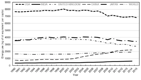
[image:1.595.312.542.365.496.2]

The energy use per capita has an increasing trend yet in terms of quantum it is very low (Figure 1). For developed countries, it is found that energy use per capita is almost constant or is having a declining trend. The energy use per capita is almost double than that of the United Kingdom or Japan. However, for clean sustainable energy use, it is advocated to be low and to have a declining trend. Measures need to be taken to provide sufficient energy to the users without detrimental to the environmental. This calls for a major shift over from the conventional sources to renewable energy sources.

Fig 1. Per capita energy consumption

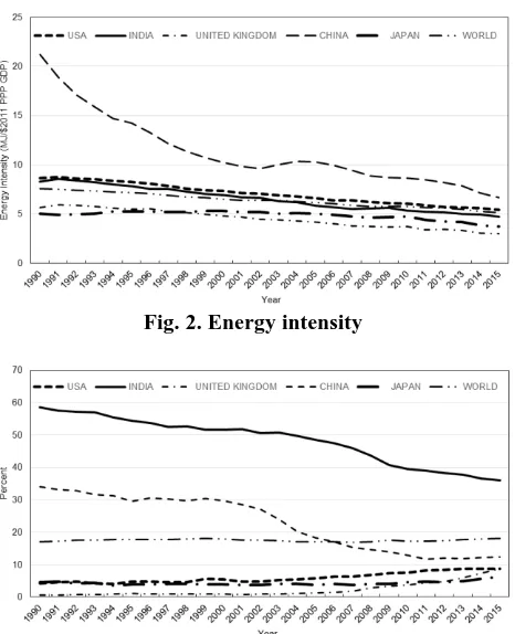
The energy intensity is compared across the various countries (Figure 2). The energy intensity is declining over the years for the Indian subcontinent. Though this is a positive sign, however, the rate of decline needs to be improved, since the rate of energy consumed needs to be far lesser against the national income of the country. This is mainly because of the large amount of fossil fuel imports. If the import of fossil fuel is restricted and to that extent, if renewable energy is used, then, far lesser energy intensity for the country will be witnessed.

The renewable energy was studied. A steady increase was witnessed. However in terms of percentage contribution, there is a decrease over the years. This is seen from the Figure 3. Measures have to be taken at a massive level so that the renewable energy is being utilized in a commercial manner and it is available to the consumers as an easy, cheap energy option. Until this happens it is very difficult. Policymakers should strategize the renewable energy utilization so that it is readily available to the common man as an alternative energy to electricity.

Renewable Energy Substitution in Lieu of Fossil

Fuel Based Energy For India

(2)

[image:2.595.54.287.47.334.2]

Fig. 2. Energy intensity

Fig. 3. Percentage of renewable energy utilization

Research has been done on how to enforce increased renewable energy utilization. Energy forecasting and optimization has been carried out to identify strategies for increasing renewable energy substitution. The energy Prediction of various fossil based energy fuels requirement is made upto 2040-41. This will help policymakers to proactively plan their requirement. Strategies are proposed to commercialize the renewable energy utilization.

II. LITERATURE REVIEW

Review of literature was undertaken in the domain of energy forecasting and optimization. The meta-analysis carried out by Suganthi and Samuel [6] highlights the energy planning models used. It includes from time series, regression and econometric models. Furthermore, autoregressive integrated moving average (ARIMA) have also been used for load forecasting wherein variations are hourly, daily and monthly. In addition soft computing tools have also been used namely particle swarm optimization (PSO), grey prediction, unit root test and co-integration models, support vector regression. Hybrid models such as artificial neural network, neuro-fuzzy, have also used.

Review indicated regression models are being used for energy forecasting [7],[8]. A hybrid model of ARIMA with particle swarm optimization has also been proposed for better forecasting accuracy [9]. To improve on the accuracy, more complex models have also been developed.

Econometric models were also being used to predict energy demand. Several researchers have worked on econometric models for prediction of energy demand [10],[11]. The supremacy of each model is presented based on their prediction accuracy.

Several soft computing techniques are also being used.

ANN has been used to predict monthly, hourly electric demand [12]. Also, vector autoregressive (VAR) models and internal multilayer perceptron (iMLP) are also being used in electric demand prediction [13]. Genetic algorithm (GA) has been used for forecasting monthly electricity demand considering population, gross domestic product and other variables [14]. Simulation process have also been explored for prediction.

Independent component analysis and ICA- SVR [15] was used for oil price prediction. Neuro-fuzzy inference system was used to forecast wind energy [16] while stochastic dual dynamic programming was used to predict hydro energy needs. The review indicated that adopting sophisticated models result in a higher degree of accuracy.

Linear optimization models [17], [18] try to optimize the different energy needs based on the energy demand. In some instances models were developed for specific energy needs, for instance.

From the review of literature the following inferences were drawn. Firstly energy return on investment that includes energy per capita and energy intensity have not been studied in detail in energy planning models. Secondly, the energy constraints of a country have to be given importance. Thirdly optimization model that considered targeted renewable energy substitution have not been developed.

These research gaps are being addressed in this research work.

III. METHODOLOGY

The data regarding energy consumption for past three decades was collected from government published statistics [2]. The constraints used in the optimization model was determined [19]. Energy return on investment was also collected [20] for various renewable energy sources.

A. Energy Forecasting

Time series models were built to find the best fit energy demand. Then using the results of time series models, econometric models were determined for 2040-41. The fossil fuel based energy requirement was found. The time series model used linear, logarithmic, power, exponential and quadratic models. The parameters used in the econometric model include

Ebest = Best fit time series energy demand.

Et-1 = Demand in the preceding year t-1.

PRi = Wholesale price index.

HC = Human capital.

NI = Gross National Product Index.

i = energy in terms of coal and lignite, oil and gas, electricity.

FER = Forecasted energy requirement.

The various models proposed are given in Table 1. Additive and multiplicative models were found totaling 91 models. The best fit is determined considering the R2, squared error and Durban Watson

(3)

[image:3.595.68.268.80.785.2]

till 2040-41 is predicted using the best fit.

Table 1. Econometric Models

Sl. No Models

1 FER = f(Ebest, PRi , NI)

2 FER = f(Et_1, PRi , NI)

3 FER = f(Ebest, PRi, NI, HC)

4 FER = f(E t-1, PRi, NI, HC)

5 FER = f(Ebest , NI)

6 FER = f(E t-1, NI)

7 FER = f(Ebest , PRi)

8 FER = f(E t-1, PRi)

9 FER = f (Ebest , HC)

10 FER = f (E t-1 , HC)

11 FER = f(PRi, NI)

12 FER = f(PRi, HC)

13 FER = f(NI, HC)

14 FER = f(Ebest , PRi, HC)

15 FER = f(E t-1, PRi, HC)

16 FER = f(Ebest , NI, HC)

17 FER = f(E t-1, NI, HC)

18 FER = f(PRi, NI, HC)

19 FER = f(Ebest , PRi/NI)

20 FER = f(E t-1, PRi/NI)

21 FER = f(Ebest , NI/PRi)

22 FER = f(E t-1, NI/PRi)

23 FER = f(Ebest , PRi/HC)

24 FER = f(E t-1, PRi/HC)

25 FER = f(Ebest , NI/HC)

26 FER = f(E t-1, NI/HC)

27 FER = f(Ebest , PRi/NI, HC)

28 FER = f(E t-1, PRi/NI, HC)

29 FER = f(Ebest , NI/PRi, HC)

30 FER = f(E t-1, NI/PRi, HC)

31 FER = f(Ebest , PRi/HC, NI)

32 FER = f(E t-1, PRi/HC, NI)

33 FER = f(Ebest , NI/HC, PRi)

34 FER = f(E t-1, NI/HC, PRi)

35 FER = f(Ebest / NI, PRi)

36 FER = f(E t-1 / NI, PRi)

37 FER = f(Ebest / NI, HC)

38 FER = f(E t-1 / NI, HC)

39 FER = f(Ebest / NI, PRi, HC)

40 FER = f(E t-1 / NI, PRi, HC)

41 FER = f (Ebest / HC, PRi)

42 FER = f(E t-1 / HC, PRi)

43 FER = f(Ebest / HC, NI)

44 FER = f(E t-1 / HC, NI)

45 FER = f(Ebest / HC, PRi, NI)

46 FER = f(E t-1 / HC, PRi, NI)

B. Optimization model

Using the fossil fuel energy requirement in 2040-41, the percentage renewable energy to be substituted is determined. An optimization model is constructed. The combination of different renewable energy sources to be utilized are determined.

Consumer acceptance, demand, potential, reliability, CO2 emissions, human capital availability and energy return on investment are the constraints. The model is run with 38 variables and 32 constraints to find the maximum amount of renewable energy distribution in 2040-41

The objective function is as follows

subject to the following constraints i.Social acceptance .. 6 constraints

ii.Demand .. 6 constraints

iii.Potential .. 6 constraints

iv.Reliability 6 constraints

v.CO2 emission .. 1 constraint

vi.Human capital availability .. 1 constraint

vii.Energy return on investment .. 6 constraints

where

 = efficiency of the system C = cost of the system D = renewable energy demand E = emission factor

EROI = energy return on investment F = employment factor

(4)

T = target emission

X = quantum of renewable energy

Subscripts

i = renewable energy system j = enduse

k = resource

n = emission from CO2

l = number of systems in respective enduses l = 5 for lighting

l = 7 for cooking l = 7 for pumping l = 7 for heating l = 6 for cooling l = 6 for transportation m = renewable energy

m = 16 for solar m = 6 for wind

m = 6 for biomass gasifier

m = 2 for biomass direct combustion m = 6 for biogas

m = 2 for ethanol

Renewable energy substitution at 40, 50 and 60% in the total energy scene has been determined. Strategies are proposed for commercial utilization of renewable energy.

IV. RESULTS

A. Prediction of Energy demand

Time series models are used to predict the fossil fuel based energy. The energy demand is predicted using year as the dependent variable. The best fit for energy demand Ebest was selected using R2 and SE.

In almost for all types of fossil based energy, quadratic equation dominated the scene indicated an exponential growth in energy consumption as shown in Appendix 1. The best fit time series model is used as one of the variables in the econometric models.

Econometric models was used with the past data to find the model equation. The variables used were best fit demand, energy price, GNP and population. The various models given in Table 1 were fitted using regression equation in SPSS. R2, SE and DW was used to validate the models. Though there are several methods used for validation, in this research these three techniques were adopted. A combined rank was used and the top ranking models identified. The details are given in Appendix 2. t-test was used to find the best fit and the results are presented in Appendix 3 for coal. Similarly it is carried out for other fossil fuel based energy sources.

[image:4.595.308.547.59.239.2]

The best fit econometric models is given in Table 2. Additive models emerged as the best fit models. Looking at the models, it is inferred that energy consumption pattern is strongly dependent on the preceding year’s energy consumption. Coal consumption is strongly dependent on price and population. Oil consumption is dependent on the national income and population. Natural gas is influenced by population and national income. Electricity consumption is dependent on national income and price.

Table 2. Best fit Econometric Model Sourc

e

Best fit Econometric Model

Coal FER = - 406808 + 0.566*(E t-1) -

4305.961*(PRi) + 1751.455*(HC)

R2 = 0.8410 SE = 70115.080 DW = 2.13 Oil FER = - 1097830 + 0.377*( E t-1) +

27949.563*(NI/HC)

R2 = 0.995 SE = 66496.02 DW = 1.451 Natura

l gas

FER = - 106930 + 646958.3*(E t-1/HC) +

2388.004*NI

R2 = 0.986 SE = 29268.12 DW = 1.866 Electri

city

FER = 56249.564 + 1.003*( E t-1) -

14413.5*(NI/PRi)

R2 = 0.998 SE = 13919.88 DW = 1.091

The energy demand is predicted until 2040-41 using the best fit model. The total fossil fuel based energy needs in 2030-31 is for coal & lignite = 23729.91 petajoule (pJ), oil =16224.78 pJ, natural gas = 2884.62 pJ and electricity=7242.38 pJ. In 2040-41 it is expected to be coal & lignite =32203.42 pJ oil =20396.92 pJ, natural gas =3460.77 pJ and electricity=9887.71 pJ. The total energy requirement in 2030-31 will be 50081 pJ and in 2040-41 it will be 65948 pJ. If this is the total energy requirement, the contribution from renewable energy sources is calculated and the results are taken as input into the optimization model.

B. Optimization model

[image:4.595.313.540.499.660.2]

The optimization model is run for 40%, 50% and 60% renewable energy penetration in 2040-41 in the total energy scene using solver add-in in Excel. If 40% of renewable energy has to be used in the total energy scene in 2040-41 the proportion of various renewable sources in different enduses have been determined and given in Figure 4.

Figure 4. Renewable energy distribution pattern in 2040-41

The results clearly indicate that solar energy utilization is the mostly preferred resource considering the various constraints. Necessary steps have to be taken to ensure solar energy utilization is

(5)

V. RECOMMENDATIONS

Considering the energy requirement in 2040-41 and the optimization plan proposed it is found that solar energy is the most optimal resource. To implement solar energy at a large scale, it is suggested that smart grid is the best solution. Implementing smart grid technology requires the support of several technologies like sensors, robotics, and advanced analytics, which together form advanced, interconnected systems. These technologies need to be capable of receiving and transferring enormous amount of data. Also it requires analysis of the data for optimally understanding the requirements and transferring the power. These systems are very sensitive and critical. They are the brain behind the smart grid operation. It needs to be flexible and agile to quickly decipher the large quantum of data getting transferred through the systems. As it processes and decides on the data the system learns and become intelligent in the process thus becoming smart. analyzing large amounts of data. Furthermore, with the advent of internet of things, there emerges a suite of technologies which aid in integrating the various devices to communicate among themselves.

In earlier days, when the electricity goes off, it was the responsibility on the part of the customer to inform the electricity board. Presently with sensors on the electricity line, when the electricity line goes off, an alert is immediately sent out. This aids in immediately rectifying the problem. Similarly when the utilities are equipped with smart gird technologies, it will help in delivering qaulity power from the grid to the consumers. Furthermore the power from the smart grid will be clean and renewable in nature. However, the communication system network is evolving. Research and development is being carried out to bring in wireless connectivity and thus offer better quality of life. With the new revolution happening in the IoT front, the comunications network is becoming an enabler of smart gird adoption. Utilities are hence able to offer more efficient customer service.

Smart grid enabled IoT offers opportunities for utilities to efficiently and effectively utilize the research innovations. The performance of the power grid using IoT enabled smart grid can be improved through three stages: (i) by collecting the data from the various devices and sensors and analyzing the data to make the grid more robust (ii) to ensure the utilities are optimally using the solar and wind energy being received from various generation points and (iii) allowing an optimal decision support system to intelligently manage and decide the energy resource to be used at a point in time for the benefit of all stakeholders [89]. As far as India is concerned we are in the evolving state. In future, a detailed study needs to be done on how to adopt smart grid technology that integrates the decentratlized renewable energy generated at sources using the IoT devices, supplies it to the grid which then distributes it back to the enduser in an optimal manner. In addition, detailed research is required to find the prevailing conditions, social acceptance, technical viability and economic feasibility of introducing smart grid with IoT devices.

VI. CONCLUSION

As expected, the results from the forecasting model indicates the energy requirement in India is going to double. Policy makers have to ensure that renewable energy sources are getting utilized to a larger extent. For this the energy from renewable sources should be easily and readily available. Also it has to be competitive with the existing electricity pricing. The optimization model indicates that solar energy is the most optied renewable energy source considerign the various constriaints. Solar energy need to be commercialized so that it is available as an alternate energy in decentralized locations. The technology in research and development stage need to moved to commercialization stage. If smart grid becomes economically and technically feasible then electricity from renewable energy can be plugged into the grid. Globally the world is marching towards advanced research in IoT device and smart grid optimization methodologies. The national status reveals that this technology is being propagated by Government of India by giving training programs and encouraging research and development activities. The research highlights the need for commercializing the renewable energy technologies and make a viable option for the consumers.

APPENDIX

Appendix 1. Best fit Time series Model.

Source Best fit Time series Model

Coal Ebest = 1043987 + 60907.8 t – 1420.3 t2

R2 = 0.7825 SE = 89256.51 Oil Ebest = 1226610.99 + 49609.66 t +

4311.96 t2

R2 ₌

0.990016 SE = 108199.1 Natural

gas

Ebest = -6105.02 + 1385.09 t + 708.69 t2

R2 = 0.9761 SE = 40249.23 Electricity

Ebest = 72405.35 – 10623.95 t – 625.91 t2

R2₌

0.991088 SE = 38178.99

Appendix 2. Top ten Econometric Models

Model Type R2 _SE _DW _Rank

Coal

FER = f(E t-1, PRi, NI, HC)

Add model

0.84115

1 70103.65 2.147477 1

FER =f(E t-1, PRi, HC)

Add model

0.84110

3 70115.08 2.125131 2

FER =f(E t-1, PRi, NI)

Add model

0.81797

1 75042.17 2.343611 3

FER =( E t-1, NI/HC, PRi)

Add model

0.81469

6 75714.14 2.267665 4

FER =f(E t-1, PRi, NI, HC)

Mult model

0.81974

7 74765.27 1.945845 5

Mult model

0.81969

4 75576.08 1.912408 6

FER =( E t-1, NI/PRi, HC)

Add model

0.82182

5 74247.11 1.873227 7

FER =( E t-1, PRi/HC, NI)

Add model

0.80961

1 76745.85 2.210422 8

Mult model

0.81562

(6)

Mult model

0.81617

2 75597.53 1.888278 10

Oil

Add model

0.99705

8 55014.18 1.590992 1

FER =( E t-1, NI/HC, PRi)

Add model

0.99645

1 60422.04 1.557119 2

FER =f(Ebest, PRi, NI, HC)

Add model

0.99584

2 66732.23 1.503687 3

FER =( E t-1, NI/HC)

Add model

0.99570

1 66496.02 1.451783 4

FER =f(E t-1/ HC, PRi, NI)

Add model

0.99640

1 60835.38 1.369393 5

FER =f(Ebest, PRi, NI)

Add model

0.99578

6 67168.47 1.448191 6

FER =f(Ebest, NI, HC)

Add model

0.99559

9 68645.52 1.50946 7

Add model

0.99647

7 60191.98 1.280157 8

FER =f(E t-1/ HC, PRi, NI)

Mult model

0.99607

4 64058.74 1.302302 9

FER =( Ebest, PRi/HC, NI)

Add model

0.99563

8 68349.25 1.401933 10

Natural gas

FER =f(E t-1 / HC, PRi, NI)

Add

model 0.98647 29267.53 1.863239 1

FER =f(E t-1/ HC, NI)

Add model

0.98646

9 29268.12 1.866548 2

FER =f( E t-1, PRi/NI, HC)

Add model

0.98521

1 30598.61 1.878257 3

FER =f( E t-1, NI/PRi, HC)

Add model

0.98573

5 30051.26 1.846731 4

FER =f(E t-1/ HC, PRi)

Add model

0.98322

4 32588.91 2.045588 5

Add model

0.98573

3 30053.72 1.803188 6

FER =f(E t-1, NI, HC)

Mult model

0.98376

1 32534.64 1.880705 7

Add

model 0.98503 30785.46 1.86288 8

Add

model 0.98527 30537.43 1.782798 9

FER =f( E t-1, NI/PRi)

Add model

0.98204

4 33715.7 1.923457 10

Electricity

Add model

0.99880

9 13690.46 1.16236 1

Add model

0.99877

1 13905.34 1.225802 2

Add model

0.99880

9 13692.23 1.160374 3

Add model

0.99880

2 13729.19 1.134825 4

FER =f(E t-1, NI/PRi, HC)

Add model

0.99879

1 13796.05 1.078435 5

FER =f(E t-1, NI/PRi)

Add model

0.99876

9 13919.88 1.091388 6

FER =f(E t-1, NI/HC, PRi)

Add model

0.99874

3 14062.7 1.197076 7

FER =f(E t-1, HC)

Add model

0.99876

7 13931.64 1.044245 8

FER =f(E t-1, NI/HC, PRi)

Mult model

0.99875

7 14049.62 1.062016 9

FER =f(E t-1, PRi/NI, HC)

Add

model 0.99877 13914.64 1.025626 10

Appendix 3. Econometric models.

CR Models for

Coal

Typ e

Variabl es

t Signif O

Ran k

1 FER = f(E t-1, PRi, NI, HC)

Add Constant -1.388 .176

E t-1 3.423 .002 PRi -2.091 .046

NI .092 .927

HC 2.021 .053

2 FER =f(E t-1, PRi, HC)

Add Constant -1.435 .162 1

E t-1 4.196 .000 PRi -2.521 .017 HC 2.523 .017 3 FER =f(E t-1,

PRi, NI)

Add Constant .497 .623

E t-1 10.480 .000

PRi -1.377 .179

NI 1.367 .182

4 FER =( E t-1, NI/HC, PRi)

Add Constant -.210 .835

E t-1 10.400 .000 NI /HC 1.150 .259

PRi -1.162 .255

5 FER =f(E t-1, PRi, NI, HC)

Mult Constant .059 .953

E t-1 5.001 .000

PRi -.038 .970

NI -.957 .347

HC .645 .524

6 FER =f(E t-1, NI, HC)

Mult Constant .319 .752

E t-1 5.100 .000

NI -1.263 .216

HC 1.276 .212

7 FER =( E t-1, NI/PRi, HC)

Add Constant 2.293 .029

E t-1 5.692 .000 NI/PRi -1.591 .123

HC -1.143 .262

8 FER =( E t-1, PRi/HC, NI)

Add Constant .882 .385

Et-1 8.590 .000

PRi/HC -.734 .469

NI .725 .474

9 FER =( E t-1, PRi/HC, NI)

Mult Constant 1.984 .057

E t-1 6.083 .000

PRi/HC 1.052 .301

NI -1.003 .324

10 FER =f(E t-1, PRi, NI)

Mult Constant 2.054 .049

E t-1 5.931 .000

PRi 1.087 .286

NI -1.047 .304

REFERENCES

1. http://energyatlas.iea.org/#!/profile/WORLD/IND. [Accessed: 10-Jun-2019].

2. http://mospi.nic.in/sites/default/files/publication_reports/Energy Statistics 2019-finall.pdf.

3. https://en.wikipedia.org/wiki/Energy_policy_of_India. [Accessed: 10-Jun-2019]. 4. https://www.bp.com/content/dam/bp/business-sites/en/global/ corporate/pdfs/energy-economics/statistical-review/bp-stats-review-2 018-full-report.pdf. 5. https://economictimes.indiatimes.com/news/politics-and-nation/ will-try-to-achieve-pledged-renewable-energy-targets-in-less-than-fou r-and-half-years-piyush-goyal/articleshow/49687054.cms. [Accessed: 10-Jun-2019].

6. L. Suganthi and A. A. Samuel, “Energy models for demand forecasting - A review,” Renew. Sustain. Energy Rev., vol. 16, no. 2, pp. 1223–1240, 2012.

7. K. B. Debnath, M. Mourshed, and S. P. K. Chew, “Modelling and Forecasting Energy Demand in Rural Households of Bangladesh,” Energy Procedia, vol. 75, pp. 2731–2737, Aug. 2015.

8. V. Dordonnat, A. Pichavant, and A. Pierrot, “GEFCom2014 probabilistic electric load forecasting using time series and semi-parametric regression models,” Int. J. Forecast., vol. 32, no. 3, pp. 1005–1011, 2016.

9. J. Wang, S. Zhu, W. Zhang, and H. Lu, “Combined modeling for electric load forecasting with adaptive particle swarm optimization,” Energy, vol. 35, no. 4, pp. 1671–1678, Apr. 2010.

10. L. Suganthi and A. A. Samuel, “Modelling and forecasting energy consumption in India: Influence of socioeconomic variables,” Energy Sources, Part B Econ. Planning, Policy, vol. 11, no. 5, pp. 404–411, May 2016.

(7)

towards achieving of China’s 2020 carbon emission reduction target—A discussion of low-carbon energy policies at province level,” Energy Policy, vol. 39, no. 5, pp. 2740–2747, May 2011.

12. M. Kankal, A. Akpınar, M. İ. Kömürcü, and T. Ş. Özşahin, “Modeling and forecasting of Turkey’s energy consumption using socio-economic and demographic variables,” Appl. Energy, vol. 88, no. 5, pp. 1927–1939, May 2011.

13. C. García-Ascanio and C. Maté, “Electric power demand forecasting using interval time series: A comparison between VAR and iMLP,” Energy Policy, vol. 38, no. 2, pp. 715–725, Feb. 2010.

14. O. E. Canyurt and H. K. Ozturk, “Application of genetic algorithm (GA) technique on demand estimation of fossil fuels in Turkey,” Energy Policy, vol. 36, no. 7, pp. 2562–2569, Jul. 2008.

15. L. Fan, S. Pan, Z. Li, and H. Li, “An ICA-based support vector regression scheme for forecasting crude oil prices,” Technol. Forecast. Soc. Change, vol. 112, pp. 245–253, Nov. 2016.

16. I. Okumus and A. Dinler, “Current status of wind energy forecasting and a hybrid method for hourly predictions,” Energy Convers. Manag., vol. 123, pp. 362–371, Sep. 2016.

17. J. T. Wilkerson, B. D. Leibowicz, D. D. Turner, and J. P. Weyant, “Comparison of integrated assessment models: Carbon price impacts on U.S. energy,” Energy Policy, vol. 76, pp. 18–31, Jan. 2015. 18. D. Lauinger, P. Caliandro, J. Van herle, and D. Kuhn, “A linear

programming approach to the optimization of residential energy systems,” J. Energy Storage, vol. 7, pp. 24–37, Aug. 2016.

19. L. Suganthi and A. Williams, “Renewable energy in India - A modelling study for 2020-2021,” Energy Policy, vol. 28, no. 15, pp. 1095–1109, 2000.

20. C. A. S. Hall, J. G. Lambert, and S. B. Balogh, “EROI of different fuels and the implications for society,” Energy Policy, vol. 64, pp. 141–152, Jan. 2014.

AUTHORSPROFILE