2005 Performance
2005 Performance
Optimization and Tuning
Handbook
Ken England
Gavin Powell
Amsterdam • Boston • Heidelberg • London • New York • Oxford Paris • San Diego• San Francisco • Singapore • Sydney • Tokyo
Linacre House, Jordan Hill, Oxford OX2 8DP, UK
Copyright © 2007, Elsevier Inc. All rights reserved.
No part of this publication may be reproduced, stored in a retrieval system, or transmitted in any form or by any means, electronic, mechanical, photocopying, recording, or otherwise, without the prior written permission of the publisher.
Permissions may be sought directly from Elsevier’s Science & Technology Rights Department in Oxford, UK: phone: (+44) 1865 843830, fax: (+44) 1865 853333, E-mail: [email protected]. You may also complete your request online via the Elsevier homepage (http://elsevier.com), by selecting “Support & Contact” then “Copyright and Permission” and then “Obtaining Permissions.”
Recognizing the importance of preserving what has been written, Elsevier prints its books on acid-free paper whenever possible.
Library of Congress Cataloging-in-Publication Data
Application Submitted.
British Library Cataloguing-in-Publication Data
A catalogue record for this book is available from the British Library.
ISBN: 978-1-55558-319-4
For information on all Elsevier Digital Press publications visit our Web site at www.books.elsevier.com
Printed in the United States of America
Introduction xv
1 Performance and SQL Server 2005 1
2. Logical Database Design for Performance 19
3. Physical Database Design 65
4. SQL Server Storage Structures 75
5. Indexing 121
6. Basic Query Tuning 193
7. What Is Query Optimization? 217
8. Investigating and Influencing the Optimizer 257
9. SQL Server and Windows 307
10. Transactions and Locking 355
11. Architectural Performance Options and Choices 409
12. Monitoring Performance 421
Appendices
A. Syntax Conventions 445
B. Database Scripts 447
C. Performance Strategies and Tuning Checklist 477
Introduction xv
1 Performance and SQL Server 2005 1
1.1 Partitioning tables and indexes 1
1.2 Building indexes online 2
1.3 Transact SQL improvements 2
1.4 Adding the .NET Framework 3
1.5 Trace and replay objects 4
1.6 Monitoring resource consumption with SQL OS 4
1.7 Establishing baseline metrics 4
1.8 Start using the GUI tools 7
1.8.1 SQL Server Management Studio 8
1.8.2 SQL Server Configuration Manager 9
1.8.3 Database Engine Tuning Advisor 9
1.8.4 SQL Server Profiler 12
1.8.5 Business Intelligence Development Studio 14
1.9 Availability and scalability 15
1.10 Other useful stuff 16
1.11 Where to begin? 17
2 Logical Database Design for Performance 19 2.1 Introducing logical database design for performance 19
2.2 Commercial normalization techniques 21
2.2.1 Referential integrity 22
2.2.2 Primary and foreign keys 23
2.2.3 Business rules in a relational database model 25
2.2.4 Alternate indexes 26
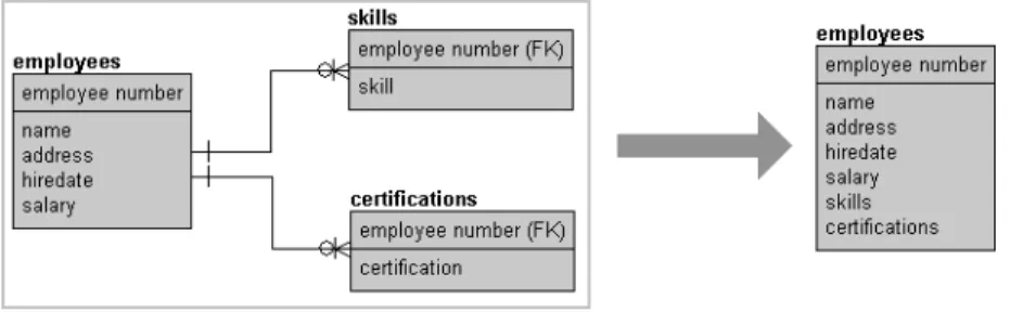
2.3.1 What is denormalization? 31
2.3.2 Denormalizing the already normalized 31
2.3.2.1 Multiple table joins (more than two tables) 32 2.3.2.2 Multiple table joins finding a few fields 32
2.3.2.3 The presence of composite keys 34
2.3.2.4 One-to-one relationships 35
2.3.2.5 Denormalize static tables 37
2.3.2.6 Reconstructing collection lists 38
2.3.2.7 Removing tables with common fields 38
2.3.2.8 Reincorporating transitive dependencies 39
2.3.3 Denormalizing by context 40
2.3.3.1 Copies of single fields across tables 40
2.3.3.2 Summary fields in parent tables 42
2.3.3.3 Separating data by activity and
application requirements 43
2.3.3.4 Local application caching 44
2.3.4 Denormalizing and special purpose objects 44
2.4 Extreme denormalization in data warehouses 48
2.4.1 The dimensional data model 51
2.4.1.1 What is a star schema? 53
2.4.1.2 What is a snowflake schema? 54
2.4.2 Data warehouse data model design basics 56
2.4.2.1 Dimension tables 57
2.4.2.2 Fact tables 60
2.4.2.3 Other factors to consider during design 63
3 Physical Database Design 65
3.1 Introducing physical database design 65
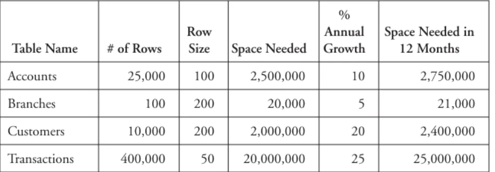
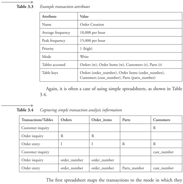
3.2 Data volume analysis 67
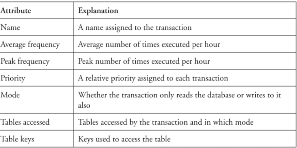
3.3 Transaction analysis 69
3.4 Hardware environment considerations 73
4 SQL Server Storage Structures 75
4.1 Databases and files 75
4.2 Creating databases 79
4.3 Increasing the size of a database 83
4.4 Decreasing the size of a database 84
4.4.1 The autoshrink database option 86
4.4.2 Shrinking a database in the SQL Server
4.4.3 Shrinking a database using DBCC statements 88
4.5 Modifying filegroup properties 90
4.6 Setting database options 92
4.7 Displaying information about databases 95
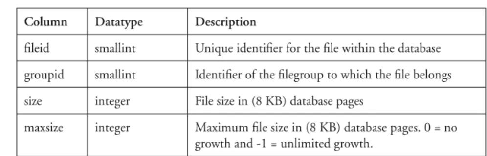
4.8 System tables used in database configuration 98
4.9 Units of storage 102
4.10 Database pages 104
4.11 Looking into database pages 108
4.12 Pages for space management 112
4.13 Partitioning tables into physical chunks 115
4.13.1 Types of partitions 117
4.13.2 Creating a range partition 117
4.13.3 Creating an even distribution partition 118
4.14 The BankingDB database 119
5 Indexing 121
5.1 Data retrieval with no indexes 121
5.2 Clustered indexes 122
5.3 Non-clustered indexes 127
5.4 Online indexes 129
5.5 The more exotic indexing forms 129
5.5.1 Parallel indexing 129
5.5.2 Partition indexing 130
5.5.3 XML data type indexes 130
5.6 The role of indexes in insertion and deletion 131
5.7 A note with regard to updates 141
5.8 So how do you create indexes? 142
5.8.1 The Transact-SQL CREATE INDEX statement 142
5.8.2 The SQL Management Studio 153
5.8.3 The SQL Distributed Management
Framework (SQL-DMF) 155
5.9 Dropping and renaming indexes 157
5.10 Displaying information about indexes 158
5.10.1 The system stored procedure sp_helpindex 158
5.10.2 The system table sysindexes 159
5.10.3 Using metadata functions to obtain information
about indexes 161
5.10.4 The DBCC statement DBCC SHOWCONTIG 163
5.11 Creating indexes on views 167
5.12 Creating indexes with computed columns 170
5.13.1 Retrieving a single row 173
5.13.2 Retrieving a range of rows 175
5.13.3 Covered queries 177
5.13.4 Retrieving a single row with a clustered index on
the table 178
5.13.5 Retrieving a range of rows with a clustered index on
the table 179
5.13.6 Covered queries with a clustered index on the table 180 5.13.7 Retrieving a range of rows with multiple non-clustered
indexes on the table 180
5.14 Choosing indexes 182
5.14.1 Why not create many indexes? 183
5.14.2 Online transaction processing versus decision support 184
5.14.3 Choosing sensible index columns 185
5.14.4 Choosing a clustered index or a non-clustered index 189
6 Basic Query Tuning 193
6.1 The SELECT statement 194
6.1.1 Filtering with the WHERE clause 195
6.1.2 Sorting with the ORDER BY clause 196
6.1.2.1 Overriding WHERE with ORDER BY 197
6.1.3 Grouping result sets 198
6.1.3.1 Sorting with the GROUP BY clause 198
6.1.3.2 Using DISTINCT 199
6.1.3.3 The HAVING clause 199
6.2 Using functions 200
6.2.1 Data type conversions 200
6.3 Comparison conditions 201
6.3.1 Equi, anti, and range 202
6.3.2 LIKE pattern matching 203
6.3.3 Set membership 204
6.4 Joins 204
6.4.1 Efficient joins 205
6.4.1.1 Intersections 205
6.4.1.2 Self joins 206
6.4.2 Inefficient Joins 207
6.4.2.1 Cartesian Products 207
6.4.2.2 Outer Joins 207
6.4.2.3 Anti-joins 209
6.4.3 How to tune a join 209
6.5.1 Correlated versus non-correlated subqueries 210
6.5.2 IN versus EXISTS 210
6.5.3 Nested subqueries 210
6.5.4 Advanced subquery joins 211
6.6 Specialized metadata objects 213
6.7 Procedures in Transact SQL 214
7 What Is Query Optimization? 217
7.1 When is a query optimized? 218
7.2 The steps in query optimization 218
7.3 Query analysis 219
7.3.1 Search arguments 219
7.3.2 OR clauses 223
7.3.3 Join clauses 224
7.4 Index selection 225
7.4.1 Does a useful index exist? 226
7.4.2 How selective is the search argument? 226
7.4.3 Key distribution statistics 227
7.4.4 Column statistics 233
7.4.5 Updating index and column statistics 234
7.4.6 When can we not use statistics? 240
7.4.7 Translating rows to logical reads 241
7.4.7.1 No index present 242
7.4.7.2 A clustered index present 242
7.4.7.3 A non-clustered index present 243
7.4.7.4 A non-clustered index present and a clustered
index present 245
7.4.7.5 Multiple non-clustered indexes present 245
7.5 Join order selection 246
7.6 How joins are processed 247
7.6.1 Nested loops joins 248
7.6.2 Merge joins 251
7.6.3 Hash joins 253
8 Investigating and Influencing the Optimizer 257
8.1 Text-based query plans and statistics 259
8.1.1 SET SHOWPLAN_TEXT { ON | OFF } 259
8.1.2 SET SHOWPLAN_ALL { ON | OFF } 260
8.1.3 SET SHOWPLAN_XML { ON | OFF } 265
8.1.5 SET STATISTICS IO { ON | OFF } 267
8.1.6 SET STATISTICS TIME { ON | OFF } 268
8.1.7 SET STATISTICS XML { ON | OFF } 270
8.2 Query plans in Management Studio 270
8.2.1 Statistics and cost-based optimization 275
8.3 Hinting to the optimizer 282
8.3.1 Join hints 283
8.3.2 Table and index hints 283
8.3.3 View hints 284
8.3.4 Query hints 285
8.4 Stored procedures and the query optimizer 289
8.4.1 A stored procedure challenge 292
8.4.1.1 Changes to the table structure 295
8.4.1.2 Changes to indexes 295
8.4.1.3 Executing update statistics 295
8.4.1.4 Aging the stored procedure out of cache 295
8.4.1.5 Table data modifications 295
8.4.1.6 Mixing data definition language and data
manipulation language statements 296
8.4.2 Temporary tables 297
8.4.3 Forcing recompilation 298
8.4.4 Aging stored procedures from cache 300
8.5 Non-stored procedure plans 301
8.6 The syscacheobjects system table 304
9 SQL Server and Windows 307
9.1 SQL Server and CPU 307
9.1.1 An overview of Windows and CPU utilization 307
9.1.2 How SQL Server uses CPU 309
9.1.2.1 Priority 309
9.1.2.2 Use of symmetric multiprocessing systems 311
9.1.2.3 Thread use 312
9.1.2.4 Query parallelism 313
9.1.3 Investigating CPU bottlenecks 314
9.1.4 Solving problems with CPU 321
9.2 SQL Server and memory 323
9.2.1 An overview of Windows virtual memory management 323
9.2.2 How SQL Server uses memory 325
9.2.2.1 Configuring memory for SQL Server 326
9.2.3 Investigating memory bottlenecks 329
9.3 SQL Server and disk I/O 335
9.3.1 An overview of Windows and disk I/O 336
9.3.2 How SQL Server uses disk I/O 339
9.3.2.1 An overview of the data cache 340
9.3.2.2 Keeping tables and indexes in cache 343
9.3.2.3 Read-ahead scans 344
9.3.2.4 Shrinking database files 346
9.3.3 Investigating disk I/O bottlenecks 348
9.3.4 Solving problems with disk I/O 352
10 Transactions and Locking 355
10.1 Why a locking protocol? 356
10.1.1 Scenario 1 356
10.1.2 Scenario 2 357
10.2 The SQL Server locking protocol 358
10.2.1 Shared and exclusive locks 358
10.2.2 Row-, page-, and table-level locking 360
10.2.2.1 When are row-level locks used? 361
10.2.2.2 When are table-level locks used? 362
10.2.3 Lock timeouts 363
10.2.4 Deadlocks 364
10.2.5 Update locks 365
10.2.6 Intent locks 367
10.2.7 Modifying the default locking behavior 367
10.2.7.1 Transaction isolation levels 368
10.2.7.2 Lock hints 369
10.2.8 Locking in system tables 373
10.2.9 Monitoring locks 374
10.2.9.1 Using the sp_lock system stored procedure 375 10.2.9.2 Using the SQL Server 2005 Management Studio 379
10.2.9.3 Using the System Monitor 381
10.2.9.4 Interrogating the syslockinfo table 383 10.2.9.5 Using the system procedure sp_who 386
10.2.9.6 The SQL Server Profiler 387
10.2.9.7 Using trace flags with DBCC 388
10.3 SQL Server locking in action 393
10.4 Uncommitted data, non-repeatable reads, phantoms, and more 398
10.4.1 Reading uncommitted data 398
10.4.2 Non-repeatable reads 399
10.4.3 Phantoms 401
10.5 Application resource locks 406
10.6 A summary of lock compatibility 407
11 Architectural Performance Options
and Choices 409
11.1 The Management Studio and the .NET Framework 410
11.2 Striping and mirroring 410
11.2.1 RAID arrays 410
11.2.2 Partitioning and Parallel Processing 411
11.3 Workflow management 411
11.4 Analysis Services and data warehousing 412
11.4.1 Data modeling techniques in SQL Server 2005 413
11.5 Distribution and replication 414
11.6 Standby failover (hot spare) 417
11.6.1 Clustered failover databases 418
11.7 Flashback snapshot databases 419
12 Monitoring Performance 421
12.1 System stored procedures 422
12.2 System monitor, performance logs, and alerts 424
12.3 SQL Server 2005 Management Studio 427
12.3.1 Client statistics 427
12.3.2 The SQL Server Profiler 428
12.3.2.1 What events can be traced? 429
12.3.2.2 What information is collected? 430
12.3.2.3 Filtering information 431
12.3.2.4 Creating an SQL Server profiler trace 431 12.3.2.5 Creating traces with stored procedures 438
12.3.3 Database Engine Tuning Advisor 442
12.4 SQL OS and resource consumption 443
A Syntax Conventions 445
B Database Scripts 447
C Performance Strategies and Tuning Checklist 477
What is the goal of tuning an SQL Server database? The goal is to improve performance until acceptable levels are reached. Acceptable levels can be defined in a number of ways. For a large online transaction processing (OLTP) application the performance goal might be to provide sub-second response time for critical transactions and to provide a response time of less than two seconds for 95 percent of the other main transactions. For some systems, typically batch systems, acceptable performance might be mea-sured in throughput. For example, a settlement system may define accept-able performance in terms of the number of trades settled per hour. For an overnight batch suite acceptable performance might be that it must finish before the business day starts.
Whatever the system, designing for performance should start early in the design process and continue after the application has gone live. Per-formance tuning is not a one-off process but an iterative process during which response time is measured, tuning performed, and response time measured again.
There is no right way to design a database; there are a number of possi-ble approaches and all these may be perfectly valid. It is sometimes said that performance tuning is an art, not a science. This may be true, but it is important to undertake performance tuning experiments with the same kind of rigorous, controlled conditions under which scientific experiments are performed. Measurements should be taken before and after any modifi-cation, and these should be made one at a time so it can be established which modification, if any, resulted in an improvement or degradation.
inappro-priate indexes and badly written queries, as well as some other contributing factors, can negatively influence the query optimizer such that it chooses an inefficient strategy.
To give you some idea of the gains to be made in this area, I once was asked to look at a query that joined a number of large tables together. The query was abandoned after it had not completed within 12 hours. The addition of an index in conjunction with a modification to the query meant the query now completed in less than eight minutes! This magnitude of gain cannot be achieved just by purchasing more hardware or by twiddling with some arcane SQL Server configuration option. A database designer or administrator’s time is always limited, so make the best use of it! The other main area where gains can be dramatic is lock contention. Removing lock bottlenecks in a system with a large number of users can have a huge impact on response times.
Now, some words of caution when chasing performance problems. If users phone up to tell you that they are getting poor response times, do not immediately jump to conclusions about what is causing the problem. Circle at a high altitude first. Having made sure that you are about to monitor the correct server, use the System Monitor to look at the CPU, disk subsystem, and memory use. Are there any obvious bottlenecks? If there are, then look for the culprit. Everyone blames the database, but it could just as easily be someone running his or her favorite game! If there are no obvious bottle-necks, and the CPU, disk, and memory counters in the System Monitor are lower than usual, then that might tell you something. Perhaps the network is sluggish or there is lock contention. Also be aware of the fact that some bottlenecks hide others. A memory bottleneck often manifests itself as a disk bottleneck.
There is no substitute for knowing your own server and knowing the normal range of System Monitor counters. Establish trends. Measure a set of counters regularly, and then, when someone comments that the system is slow, you can wave a graph in front of him or her showing that it isn’t!
Also there are special thanks to be made to Craig Mullins for his work on technical editing of this book.
So, when do we start to worry about performance? As soon as possible, of course! We want to take the logical design and start to look at how we should transform it into an efficient physical design.
Gavin Powell can be contacted at the following email address:
1
Performance and SQL Server 2005
1.1
Partitioning tables and indexes
Partitioning lets you split large chunks of data in much more manageable smaller physical chunks of disk space. The intention is to reduce I/O activ-ity. For example, let’s say you have a table with 10 million rows and you only want to read 1 million rows to compile an analytical report. If the table is divided into 10 partitions, and your 1 million rows are contained in a sin-gle partition, then you get to read 1 million rows as opposed to 10 million rows. On that scale you can get quite a serious difference in I/O activity for a single report.
SQL Server 2005 allows for table partitioning and index partitioning. What this means is that you can create a table as a partitioned table, defin-ing specifically where each physical chunk of the table or index resides.
SQL Server 2000 partitioning was essentially manual partitioning, using multiple tables, distributed across multiple SQL Server computers. Then a view (partition view) was created to overlay those tables across the servers. In other words, a query required access to a view, which contained a query, not data. SQL Server 2005 table partitions contain real physical rows.
Physically partitioning tables and indexes has a number of benefits:
Data can be read from a single partition at once, cutting down enor-mously on performance hogging I/O.
Data can be accessed from multiple partitions in parallel, which gets things done at double the speed, depending on how many processors a server platform has.
1.2
Building indexes online
Building an index online allows the table indexed against to be accessed during the index creation process. Creating or regenerating an index for a very large table can consume a considerable period of time (hours, days). Without online index building, creating an index puts a table offline. If that is crucial to the running of a computer system, then you have down time. The result was usually that indexes are not created, or never regenerated.
Even the most versatile BTree indexes can sometimes require rebuilding to increase their performance. Constant data manipulation activity on a table (record insert, update and deletions) can cause a BTree index to deteri-orate over time. Online index building is crucial to the constant uptime required by modern databases for popular websites.
1.3
Transact SQL improvements
Transact SQL provides programmable access to SQL Server. Programmable access means that Transact SQL allows you to construct database stored code blocks, such as stored procedures, triggers, and functions. These code blocks have direct access to other database objects—most significantly tables where query and data manipulation commands can be executed directly in the stored code blocks; and code blocks are executed on the data-base server. New capabilities added to Transact SQL in SQL Server 2005 are as follows:
Error handling
Recursive queries
Better query writing capabilities
There is also something new to SQL Server 2005 called Multiple Active Result Sets (MARS). MARS allows for more than a single set of rows for a single connection. In other words, a second query can be submitted to a SQL Server while the result set of a first query is still being returned from database server to client application.
1.4
Adding the .NET Framework
You can use programming languages other than just Transact SQL and embed code into SQL Server as .NET Framework executables. These pro-graming languages can leverage existing personnel skills. Perhaps more importantly, some tasks can be written in programming languages more appropriate to a task at hand. For example a language like C# can be used, letting a programmer take advantage of the enormous speed advantages of writing executable code using the C programming language.
Overall, you get support for languages not inherently part of SQL Server (Transact SQL). You get faster and easier development. You get to use Web Services and XML (with Native XML capabilities using XML data types). The result is faster development, better development, and hopefully better over database performance in the long run.
The result you get is something called managed code. Managed code is code executed by the .NET Framework. As already stated, managed code can be written using all sorts of programming languages. Different pro-gramming languages have different benefits. For example, C is fast and effi-cient, where Visual Basic is easier to write code with but executes slower. Additionally, the .NET Framework has tremendous built-in functionality. .NET is much, much more versatile and powerful than Transact SQL.
There is much to be said for placing executable into a database, on a database server such as SQL Server. There is also much to be said against this practice. Essentially, the more metadata and logic you add to a data-base, the more business logic you add to a database. In my experience, add-ing too much business logic to a database can cause performance problems in the long run. After all, application development languages cater to num-ber crunching and other tasks. Why put intensive, non-data access process-ing into a database? The database system has enough to do just in keepprocess-ing your data up to date and available.
Managed code also compiles to native code, or native form in SQL Server, immediately prior to execution. So, it should execute a little faster because it executes in a form which is amenable to best performance in SQL Server.
1.5
Trace and replay objects
Tracing is the process of producing large amounts of log entry information during the process of normal database operations. However, it might be prudent to not choose tracing as a first option to solving a performance issue. Tracing can hurt performance simply because it generates lots of data. The point of producing trace files is to aid in finding errors or performance bottlenecks, which cannot be deciphered by more readily available means. So, tracing quite literally produces trace information. Replay allows replay of actions that generated those trace events. So, you could replay a sequence of events against a SQL Server, without actually changing any data, and reproduce the unpleasant performance problem. And then you could try to reanalyze the problem, try to decipher it, and try to resolve or improve it.
1.6
Monitoring resource consumption with SQL OS
SQL OS is a new tool for SQL Server 2005, which lives between an SQL Server database and the underlying Windows operating system (OS). The operating system manages, runs, and accesses computer hardware on your database server, such as CPU, memory, disk I/O, and even tasks and sched-uling. SQL OS allows a direct picture into the hardware side of SQL Server and how the database is perhaps abusing that hardware and operating sys-tem. The idea is to view the hardware and the operating system from within an SQL Server 2005 database.
1.7
Establishing baseline metrics
An established baseline metric is a measure of normal or acceptable activity.
Metric baselines have more significance (there are more metrics) in SQL Server 2005 than in SQL Server 2000. The overall effect is that an SQL Server 2005 database is now more easily monitored, and the prospect of some automated tuning activities becomes more practical in the long term. SQL Server 2005 has added over 70 additional baseline measures applicable to performance of an SQL Server database. These new baseline metrics cover areas such as memory usage, locking activities, scheduling, network usage, transaction management, and disk I/O activity.
The obvious answer to a situation such as this is that a key index is dropped, corrupt, or deteriorated. Or a query could be doing something unexpected such as reading all rows in a very large table.
Using metrics and their established baseline or expected values, one can perform a certain amount of automated monitoring and detection of per-formance problems.
Baseline metrics are essentially statistical values collected for a set of metrics.
A metric is a measure of some activity in a database.
The most effective method of gathering those expected metric values is to collect multiple values—and then aggregate and average them. And thus the term statistic applies because a statistic is an aggregate or average value, resulting from a sample of multiple values. So, when some activity veers away from previously established statistics, you know that there could be some kind of performance problem—the larger the variation, the larger the potential problem.
Baseline metrics should be gathered in the following activity sectors:
High load: Peak times (highest database activity)
Low load: Off peak times (lowest database activity)
Batch activity: Batch processing time such as during backup process-ing and heavy reportprocess-ing or extraction cycles
Some very generalized categories areas of metric baseline measurement are as follows:
Applications database access: The most common performance problems are caused by poorly built queries and locking or hot blocks (conflict caused by too much concurrency on the same data).
In computer jargon, concurrency means lots of users accessing and changing the same data all at the same time. If there are too many concurrent users, ultimately any relational database has its lim-itations on what it can manage efficiently.
Internalized database activity: Statistics must not only be present but also kept up to date. When a query reads a table, it uses what’s called an optimizer process to make a wild guess at what it should do. If a table has 1 million rows, plus an index, and a query seeks 1 record, the optimizer will tell the query to read the index. The opti-mizer uses statistics to compare 1 record required, within 1 million rows available. Without the optimizer 1 million rows will be read to find 1 record. Without the statistics the optimizer cannot even hazard a guess and will probably read everything. If statistics are out of date where the optimizer thinks the table has 2 rows, but there are really 1 million, then the optimizer will likely guess very badly.
Internalized database structure: Too much business logic, such as stored procedures or a highly over normalized table structure, can ultimately cause overloading of a database, slowing performance because a database is just a little too top heavy.
Database configuration: An OLTP database accesses a few rows at a time. It often uses indexes, depending on table size, and will pass very small amounts of data across network and telephone cables. So, an OLTP database can be specifically configured to use lots of mem-ory—things like caching on client computers and middle tier servers (web and application servers), plus very little I/O. A data warehouse on the other hand produces a small number of very large transac-tions, with low memory usage, enormous amounts of I/O, and lots of throughput processing. So, a data warehouse doesn’t care too much about memory but wants the fastest access to disk possible, plus lots of localized (LAN) network bandwidth. An OLTP database uses all hardware resources and a data warehouse uses mainly I/O.
improved upon. In some circumstances beefing up hardware will solve performance issues. For example, an OLTP database server needs plenty of memory, whereas a data warehouse does well with fast disks, and perhaps multiple CPUs with partitioning for rapid parallel processing. Beefing up hardware doesn’t always help. Sometimes increasing CPU speed and number, or increasing onboard memory, can only hide performance problems until a database grows in physi-cal size, or there are more users—the problem still exists. For exam-ple, poor query coding and indexing in an OLTP database will always cause performance problems, no matter how much money is spent on hardware. Sometimes hardware solutions are easier and cheaper, but often only a stopgap solution.
Network design and configuration: Network bandwidth and bot-tlenecks can cause problems sometimes, but this is something rarely seen in commercial environments because the network engineers are usually prepared for potential bandwidth requirements.
The above categories are most often the culprits of the biggest perfor-mance issues. There are other possibilities, but they are rare and don’t really warrant mentioning at this point. Additionally, the most frequent and exac-erbating causes of performance problems are usually the most obvious ones, and more often than not something to do with the people maintaining and using the software, inadequate software, or inadequate hardware. Hardware is usually the easiest problem to fix. Fixing software is more expensive depending on location of errors in database or application software. Per-suading users to use your applications and database the way you want is either a matter of expensive training, or developers having built software without enough of a human use (user friendly) perspective in mind.
1.8
Start using the GUI tools
1.8.1
SQL Server Management Studio
The SQL Server Management Studio is a new tool used to manage all the facets of an SQL Server, including multiple databases, tables, indexes, fields, and data types, anything you can think of. Figure 1.1 shows a sample view of the SQL Server Management Studio tool in SQL Server 2005.
SQL Server Management Studio is a fully integrated, multi-task ori-ented screen (console) that can be used to manage all aspects of an SQL Server installation, including direct access to metadata and business logic, integration, analysis, reports, notification, scheduling, and XML, among other facets of SQL Server architecture. Additionally, queries and scripting can be constructed, tested, and executed. Scripting also includes versioning control (multiple historical versions of the same piece of code allow for backtracking). It can also be used for very easy general database mainte-nance.
SQL Server Management Studio is in reality wholly constructed using something called SQL Management Objects (SMO). SMO is essentially a very large group of predefined objects, built-in and reusable, which can be used to access all functionality of a SQL Server database. SMO is written using the object-oriented and highly versatile .NET Framework. Database Figure 1.1
administrators and programmers can use SMO objects in order to create their own customized procedures, for instance, to automate something like daily backup processing.
SMO is an SQL Server 2005 updated and more reliable version of Dis-tributed Management Objects (DMO), as seen in versions of SQL Server prior to SQL Server 2005.
1.8.2
SQL Server Configuration Manager
The SQL Server 2005 Configuration Manager tool allows access to the operating system level. This includes services such as configuration for cli-ent application access to an SQL Server database, as well as access to data-base server services running on a Windows server. This is all shown in Figure 1.2.
1.8.3
Database Engine Tuning Advisor
The SQL Server 2005 Database Engine Tuning Advisor tool is just that, a tuning advisor used to assess options for tuning the performance of an SQL Figure 1.2
Server database. This tool includes both a Graphical User Interface in Win-dows and a command line tool called dta.exe.
This book will focus on the GUI tools as they are becoming more prom-inent in recent versions of all relational databases,
The SQL Server 2005 Database Engine Tuning Advisor includes other tools from SQL Server 2000, such as the Index Tuning Wizard. However, SQL Server 2005 is very much enhanced to cater to more scenarios and more sensible recommendations. In the past, recommendations have been basic at best, and even wildly incorrect. Also, now included are more object types including differentiating between clustered and non-clustered indexing, plus indexing for view, and of course partitioning and parallel processing.
The Database Engine Tuning Advisor is backwardly compatible with previous versions of SQL Server.
New features provided by the SQL Server 2005 Database Engine Tun-ing Advisor tool are as follows:
Multiple databases: Multiple databases can be accessed at the same time.
More objects types: As already stated, more object types can be tuned. This includes XML, XML data types, and partitioning recom-mendations. There is also more versatility in choosing what to tune and what to recommend for tuning. Figure 1.3 shows available options for differing object types allowed to be subjected to analysis.
And there are also some advanced tuning options as shown in Figure 1.4.
Time period workload analysis: Workloads can be analyzed over set time periods, thus isolating peak times, off-peak times, and so on. Figure 1.5 shows analysis, allowance of time period settings, as well as application and evaluation of recommendations made by the tool.
Tuning log entries: A log file containing a record of events which the Database Engine Tuning Advisor cannot tune automatically. This log can be use by a database administrator to attempt manual tuning if appropriate.
in order to offload performance tuning testing processing. Most importantly, the test database created does not copy data. The only thing copied is the state of a database without the actual data. This is actually very easy for a relational database like SQL Server. All that is Figure 1.3
Object types to tune in the Database Engine Tuning Advisor
Figure 1.4
copied are objects, such as tables and indexes, plus statistics of those objects. Typical table statistics include record counts and physical size. This allows a process such as the optimizer to accurately estimate how to execute a query.
What-if scenarios: A database administrator can create a configura-tion and scenario and subject it to the Database Engine Tuning Advi-sor. The advisory tool can give a response as to the possible effects of specified configuration changes. In other words, you can experiment with changes, and get an estimation of their impact, without making those changes in a production environment.
1.8.4
SQL Server Profiler
The SQL Server Profiler tool was available in SQL Server 2000 but has some improvements in SQL Server 2005. Improvements apply to the recording of things or events, which have happened in the database, and the ability to replay those recordings. The replay feature allows repetition of problematic scenarios which are difficult to resolve.
Essentially, the SQL Server Profiler is a direct window into trace files. Trace for any relational database contain a record of some, most, or even all activities in a database. Trace files can also include general table and index-ing statistics as well. Performance issues related to trace files themselves is that tracing can be relatively intensive, depending on how tracing is config-ured. Sometimes too much tracing can affect overall database performance, Figure 1.5
and sometimes even quite drastically. Tracing is usually a last resort but also a very powerful option when it comes to tracking down the reason for per-formance problems and bottlenecks.
There are a number of things new to SQL Server 2005 for SQL Server Profiler:
Trace file replays: Rollover trace files can be replayed. Figure 1.6 shows various options that can be set for tracing, rollover, and subse-quent tracing entry replay.
XML: The profiler tool has more flexibility by allowing for various definitions using XML.
Query plans in XML: Query plans can be stored as XML allowing for viewing without database access.
Trace entries as XML: Trace file entries can be stored as XML allow-ing for viewallow-ing without database access.
Figure 1.6
Analysis Services: SQL Server Profiler now allows for tracing of Analysis Services (SQL Server data warehousing) and Integration Ser-vices.
Various other things: Aggregate views of trace results and Perfor-mance Monitor counters matched with SQL Server database events. The Windows Performance Monitor tool is shown in Figure 1.7.
1.8.5
Business Intelligence Development Studio
This tool is used to build something called Business Intelligence (BI) objects. The BI Development Studio is a new SQL Server 2005 tool used to manage projects for development. This tool allows for integration of various aspects of SQL Server databases, including analysis, integration, and report-ing services. This tool doesn’t really do much for database performance in general, but moreover can help to speed up development, and make devel-opment a cleaner and better coded process. In the long term, better built applications perform better.
Figure 1.7
1.9
Availability and scalability
Availability means that an SQL Server database will have less down time and is less likely to irritate your source of income—your customers. Scal-ability means you can now service more customers with SQL Server 2005. Availability and scalability are improved in SQL Server 2005 by the addi-tion and enhancement of the following:
Data mirroring: Addition hot standby databases. This is called data-base mirroring in SQL Server.
Clustering: Clustering is introduced which is not the same thing as a hot standby. A hot standby takes over from a primary database, in the event that the primary database fails. Standby is purely failover abil-ity. A clustered environment provides more capacity and up-time by allowing connections and requests to be serviced by more than one computer in a cluster of computers. Many computers work in a clus-ter, in concert with each other. A cluster of multiple SQL Server data-bases effectively becomes a single database spread across multiple locally located computers—just a much larger and more powerful database. Essentially, clustering provides higher capacity, speed through mirrored and parallel databases access, in addition to just failover potential. When failover occurs in a clustered environment the failed node is simply no longer servicing the needs of the entire cluster, whereas a hot standby is a switch from one server to another.
Replication: Replication is enhanced in SQL Server 2005. Workload can be spread across multiple, distributed, replicated databases. Also the addition of a graphical Replication Monitor tool eases manage-ment of replication and distributed databases.
Snapshot flashbacks: A snapshot is a picture of a database, frozen at a specific point in time. This allows users to go back in time, and look at data at that point in time in the past. The performance benefit is that the availability of old data sets, in static databases, allows queries to be executed against multiple sets of the same data.
Backup and restore: Improved restoration using snapshots to enhance restore after crash recovery, and giving partial, general online access, during the recovery process.
1.10
Other useful stuff
Other useful stuff introduced in SQL Server 2005 offers the potential of improving the speed of development and software quality. Improvements include the following:
Native XML data types: Native XML allows the storage of XML doc-uments in their entirety inside an SQL Server database. The term Native implies that that stored XML document is not only stored as the textual data of the XML document, but it also includes the browser interpretive XML structure and metadata meaning. In other words, XML data types are directly accessible from the database as fully executable XML documents. The result is the inclusion of all the power, versatility, and performance of XML in general—ALL OF IT! Essentially, XML data types allow direct access to XQuery, SOAP, XML data manipulation languages, XSD—anything and everything XML. Also included are specifics of XML exclusive to SQL Server [1].
XML is the eXtensible Markup Language. There is a whole host of stuff added to SQL Server 2005 with the introduction of XML data types. You can even create specific XML indexes, indexing stored XML data type and XML documents.
Service broker notification: This helps performance enormously because multiple applications are often tied together in eCommerce architectures. The Server Broker part essentially organizes messages between different things. The notification part knows what to send, and where. For example, a user purchases a book online at the Ama-zon website. What happens? Transactions are placed into multiple different types of databases:
stock inventory databases
shipping detail databases
payment processing such as credit cards or a provider like Paypal
data warehouse archives
accounting databases
The different targets for data messages are really dependent on the size of the online operation. The larger the retailer, the more distrib-uted their architecture becomes. This stuff is just too big to manage all in one place.
This type of feature helps performance in terms of overall end-user pro-ductivity, rather than SQL Server database performance specifically.
1.11
Where to begin?
Essentially, when looking at database performance, it is best to start at the beginning. Where is the beginning of a relational database? The data model logical design is the where a relational database is first created. The next chapter will examine relational data model design, as applied to improving overall SQL Server database performance.
1.12
Endnotes
2
Logical Database Design for Performance
In database parlance, logical design is the human perceivable organization of the slots into which data is put. These are the tables, the fields, data types, and the relationships between tables. Physical design is the underly-ing file structure, within the operatunderly-ing system, out of which a database is built as a whole. This chapter covers logical database design. Physical design is covered in the next chapter.
This book is about performance. Some knowledge of logical relational database design, plus general underlying operating system and file system structure, and file system functioning is assumed. Let’s begin with logical database design, with database performance foremost in mind.
2.1
Introducing logical database design for
performance
Logical database design for relational databases can be divided into a num-ber of distinct areas:
Normalization: A sequence of steps by which a relational database model is both created and improved upon. The sequence of steps involved in the normalization process is called normal forms. Each normal form improves the previous one. The objective is to remove redundancy and duplication, plus reduce the chance of inconsisten-cies in data and increase the precision of relationships between differ-ent data sets within a database.
per-formance. The extreme in denormalization helps to create specialized data models in data warehouses.
Object Design: The advent of object databases was first expected to introduce a new competitor to relational database technology. This did not happen. What did happen was that relational databases have absorbed some aspects of object modeling, in many cases helping to enhance the relational database model into what is now known as an object-relational database model.
Objects stored in object-relational databases typically do not enhance relational database performance, but rather enhance functionality and ver-satility.
To find out more about normalization [1] and object design [2] you will have to read other books as these topics are both very comprehensive all by themselves. There simply isn’t enough space in this book. This book deals with performance tuning. So, let’s begin with the topic of normalization, and how it can be both used (or not used) to help enhance the performance of a relational database in general.
So, how do we go about tuning a relational database model? What does normalization have to do with tuning? There are a few simple guidelines to follow and some things to watch out for:
Normalization optimizes data modification at the possible expense of data retrieval. Denormalization is just the opposite, optimizing data retrieval at the expense of data modification.
Too little normalization can lead to too much duplication. The result could be a database that is bigger than it should be, resulting in more disk I/O. Then again, disk space is cheap compared with processor and memory power.
Incorrect normalization is often made obvious by convoluted and complex application code.
Too much normalization leads to overcomplex SQL code which can be difficult, if not impossible, to tune. Be very careful implementing beyond 3rd normal form in a commercial environment.
Too many tables results in bigger joins, which makes for slower queries.
basis. Later in the development cycle, applications may have diffi-culty mating to a highly granular data model (highly normalized). One possible answer is that both development and administration people should be involved in data modeling. Busy commercial devel-opment projects rarely have spare time to ensure that absolutely everything is taken into account. It’s just too expensive. It should be acceptable to alter the data model at least during the development process, possibly substantially. Most of the problems with relational database model tuning are normalization related.
Normalization should be simple because it is simple! Don’t overcom-plicate it. Normalization is somewhat based on mathematical set the-ory, which is very simple mathematics.
Watch out for excessive use of outer joins in SQL code. This could mean that your data model is too granular. You could have overused the higher normal forms. Higher normal forms are rarely needed in the name of efficiency, but rather preferred in the name of perfection, and possibly overapplication of business rules into database defini-tions. Sometimes excessive use of outer joins might be akin to: Go and get this. Oh! Go and get that too because this doesn’t quite cover it.
The other side of normalization is of course denormalization. In many cases, denormalization is the undoing of normalization. Normalization is performed by the application of normal form transformations. In other cases, denormalization is performed through the application of numerous specialized tricks. Let’s begin with some basic rules for normalization in a modern commercial environment.
2.2
Commercial normalization techniques
highly of a data warehouse dimensional model, which is essentially denor-malized up the gazoo! Each approach has its role to play in the constant dance of trying to get things right and turn a profit.
2.2.1
Referential integrity
How referential integrity and tuning are related is twofold:
Implement Referential Integrity? Yes. Too many problems and issues can arise if not.
How to Implement Referential Integrity? Use built-in database constraints if possible. Do not use triggers or application coding. Triggers can especially hurt performance. Application coding can cause much duplication when distributed. Triggers are event driven, and thus by their very definition cannot contain transaction termina-tion commands (COMMIT and ROLLBACK commands). The result is that their over use can result in a huge mess, with no transac-tion terminatransac-tion commands.
Some things to remember:
Always Index Foreign Keys: This helps to avoid locking contention on small tables when referential integrity is validated. Why? Without indexes on foreign key fields, every referential integrity check against a foreign key will read an entire table without the index to read. Unfavorable results can be hot blocking on small tables and too much I/O activity for large tables.
Note: A hot block is a section of physical disk or memory with excessive activity—more than the software or hardware can handle.
2.2.2
Primary and foreign keys
Using surrogates for primary and foreign keys can help to improve perfor-mance. A surrogate key is a field added to a table, usually an integer sequence counter, giving a unique value for a record in a table. It is also totally unrelated to the content of a record, other than just uniqueness for that record.
Primary and foreign keys can use natural values, effectively names or codes for values. For example, in Figure 2.1, primary keys and foreign keys are created on the names of companies, divisions, departments, and employees. These values are easily identifiable to the human eye but are lengthy and complex string values as far as a computer is concerned. People do not check referential integrity of records, the relational database model is supposed to do that.
The data model in Figure 2.1 could use coded values for names, making values shorter. However, years ago, coded values were often used for names in order to facilitate easier typing and selection of static values—not for the purpose of efficiency in a data model. For example, it is much easier to type
USA (or select it from a pick list), rather than United States of America,
when typing in a client address.
The primary and foreign keys, denoted in Figure 2.1 as PK and FK respectively, are what apply referential integrity. In Figure 2.1, in order for a division to exist it must be part of a company. Additionally, a company can-not be removed if it has an existing division. What referential integrity does is verify that these conditions exist whenever changes are attempted to any of these tables. If a violation occurs an error will be returned. It is also pos-Figure 2.1
sible to cascade or pass changes down through the hierarchy. In other words, when cascade deleting a company all divisions, departments, and employees for that company will be removed from the database, as well as the company itself.
In a purist’s or traditional relational data model, keys are created on actual values, such as those shown in Figure 2.1. The primary key for the Company table is created on the name of the company, a variable length string. Try to create keys on integer values. Integer values make for more efficient keys than alphanumeric values. This is because both range and exact searches, using numbers, are mathematically much easier than using alphanumeric values. There are only 10 possible digits to compare (0 to 9), but many more alphanumeric characters than just 10. Sorting and particu-larly hashing are much more efficient with numbers.
Avoid creating keys on large fixed or variable length strings. Dates can also cause problems due to implicit conversion requirements, and differ-ences between dates and timestamps. Numbers require less storage and thus shorter byte lengths. The only negative aspect is that as the numbers grow, predicting space occupied becomes more difficult.
A possibly more efficient key structure for the data model in Figure 2.1 would be as shown in Figure 2.2. In Figure 2.2, all variable length strings are relegated as details of the table, by the introduction of integer primary keys. Integer primary keys are known as surrogate keys, the term surrogate
meaning substitute value or key.
A more effective form of the data model shown in Figure 2.1 and Figure 2.2 would be the data model as shown in Figure 2.3. In Figure 2.3, the rela-tionships become non-identifying.
Figure 2.2
An identifying relationship exists where a parent table primary key is part of a child table primary key (the parent identifies each child directly). A parent table primary key, which is not part of the primary key in a child table, makes the relationship non-identifying. This is because each record in the child is not directly and exclusively identified by the primary key in the parent table.
In Figure 2.3, all foreign keys have been removed from the composite primary keys, resulting in a single unique primary key surrogate key field. This is often the most effective structure for an OLTP database. However, where there is heavy reporting, it can sometimes be beneficial to retain composite indexing structures like this, but perhaps as alternate keys and not as part of the primary key.
In most relational databases, surrogate keys are most efficiently gener-ated using autonomous sequence counter objects, or auto counters.
2.2.3
Business rules in a relational database model
Business rules are the rules defining both database metadata structure, and some of the data manipulation coding (commonly seen in application cod-ing—not in the database model). The idea of modern relational databases, such as SQL Server, is that you do have the option of implementing all business rules pertaining to a set of data, and large parts of the noncustomer facing part of applications, within a database model. This does not mean that you should do so.
Business rules can be implemented in a relational database model using the combination of tables, fields, data types, relationships between tables, procedures, triggers, specialized objects, and so on.
Figure 2.3
What are business rules? This term is often used vaguely where it could quite possibly have different meanings. Some technical people will insist on placing all business rules into a database. Others will insist on the opposite. Either approach is often dependent on available skills of personnel working on a particular project.
There are two important areas with respect to business rule implementa-tion inside a relaimplementa-tional database model:
Referential Integrity: Referential integrity can be implemented in the database using constraints, triggers, or application coding. Usu-ally the best option is use of constraints because they are centralized and simplistic.
SQL code: Using stored procedures, functions, and sometimes triggers.
You can put as much as you want of the business rules of an application, into a database model. Sometimes this can work well for performance. In a practical situation it makes the database model just too complex. It is better to divide up structural and processing requirements between database and application coding. There is a very simple reason for this: application cod-ing is much more proficient at processcod-ing data than any database is.
A database is primarily built to both store data and to read and write data. A database is not built to process data.
The term process means to change data from one thing into another. This function is often called number-crunching in the case of complex numerical calculations.
An application coding tool is built to process data, not store it. In short, use the appropriate tools in the appropriate places. This is fundamental to building applications and databases with acceptable performance.
2.2.4
Alternate indexes
Alternate indexes are usually created because the primary and foreign key indexes in a data model do not cater to everything required by applica-tions. That everything would be any kind of filtering and sorting, particu-larly in SQL statements, such as queries. Filtering and sorting SQL statements is what uses indexes. Those indexes help applications to access the database quickly, scanning over much smaller amounts of physical disk space, than when reading an entire table.
A database with too many alternate indexes will have more to maintain. For example, whenever a record in a table is changed, every index created against that table must be changed at the same time. So, inserting a single record into a table with four indexes in reality requires four index additions and one table addition. That is a total of five additions, not a single addi-tion. That’s a lot of work for a database to do. That can hurt performance, sometimes very badly. On the contrary, if a database has a large number of alternate indexes, there could be a number of reasons, but not necessarily all performance friendly scenarios:
Reporting in an OLTP database: More traditional relational data-base structures, such as those shown in Figure 2.1 and Figure 2.2, include composite primary keys. Composite primary keys get a little too precise and are more compatible with reporting efficiency and perhaps only a very few specific reports. Structures such as that shown in Figure 2.3 do not have composite primary keys. Imposition of reporting requirements on the structure in Figure 2.3 would probably require composite alternate indexes, somewhat negating the useful-ness of surrogate keys.
Matching query filtering and sorting with existing keys: When existing composite primary keys do not cater to requirements then perhaps either further normalization or denormalization is a possibil-ity. Or perhaps current structures simply do not match application requirements. However, changing the data model at a late stage (post-development) is difficult. Also, further normalization can cause other problems, particularly with recoding of application and stored proce-dure code.
Surrogate keys do not negate uniqueness requirements: When using surrogate keys, such as in Figure 2.3, items such as names of people or departments may be required to be unique. These unique keys are not part of referential integrity but they can be important and are most easily maintained at the database level using unique alternate indexes.
There is no cut-and-dry answers to which alternate keys should be allowed, and how many should be created. The only sensible approach is to keep control of the creation of what are essentially extra keys. These keys were not thought about in the first place. Or perhaps an application designed for one thing has been expanded to include new functionality, such as reporting.
Alternate indexing is not part of the normalization process. It should be somewhat included at the data model design stage, if only to avoid difficul-ties when coding. Programmers may swamp database administrators with requests for new indexes, if those indexes were not added when the data model was first created. Typically, alternate keys added in the data modeling stage are those most obvious as composites, where foreign keys are inherited from parent tables, such as the composite primary keys shown in Figure 2.1 and Figure 2.2.
Composite field keys use up a lot of physical space, somewhat negating the space saving I/O advantage of creating an index in the first place. Also, a composite index will create a more complicated index. A more complicated index makes the job of specialized index searching algorithms a more diffi-cult task.
architecture would be OLTP plus data warehouse architecture in separate databases, on different computers. Unless of course you prefer to spend a small fortune on fancy computer hardware.
2.3
Denormalization for performance
Before we get to data warehouse data modeling, you need to have a brief understanding of what denormalization is. A large part of denormalization is a process of undoing normalization. This is a process of removal of too much data model granularity. Too much granularity may be preventing acceptable performance of data retrieval from a relational data model. This is true not only for reporting and data warehouse databases, but also quite significantly even for OLTP databases.
In SQL Server the SQL Analysis Server is effectively a data warehousing query analysis tool.
So, as already stated, denormalization is largely a process of undoing normalization. However, that does not cover all practical possibilities. Here are some areas of interest when it comes to undoing of granularity, in addi-tion to that of undoing of normalizaaddi-tion:
Denormalization: Undoing various normal forms, some more than others.
Context: Various tricks to speed up data access based on the context of data or application function.
Denormalization using unusual database objects: Creation of spe-cial types of database objects used to cluster, pre-sort, and pre-con-struct data. These specialized objects help to avoid excessive amounts of complex repetitive SQL.
database is only most effective for single record insert, update, and deletion transactions; changing single data items.
In the past I have even seen some very poorly performing OLTP appli-cations, even those with small transactional units. The reason for this poor performance is often the result of severely granular data models. Some of these systems did not contain large numbers of records or occupy a lot of physical space. Even so, brief data selection listings into one page of a browser, more often than not performed join queries comprising many tables.
These types of applications sometimes fail, their creators fail or both. In these cases, there is a very strong case to be said for the necessity of design-ing a data model with the functionality of the application in mind, and not just the beauty of the granularity of an enormously overnormalized rela-tional data model structure.
One particular project I have in mind had some queries with joins con-taining in excess of 15 tables, a database under 10 megabytes in size, and some query return times of over 30 seconds on initial testing. These time tests were reduced to mere seconds after extensive application code changes of embedded SQL code (to get around an impractically over normalized table structure). However, it was too late to change the data model without extensive application recoding, and thus some very highly tuned and con-voluted embedded SQL code remained. Maintenance for this particular application will probably be a nightmare, if it is even possible. In a situation such as this, it might even be more cost effective to rewrite.
In conclusion, normalization granularity can often be degraded in order to speed up SQL data retrieval performance. How do we do this? The easi-est and often the most effective method, from the perspective of the data model, is a drastic reduction to the number tables in joins. It is possible to tune SQL statements joining 15 tables but it is extremely difficult—not only to write SQL code but also for the database optimizer to perform at its best. If the data model can possibly be changed then begin with that data model. Changing the data model obviously affects any SQL code, be it in stored procedures or embedded in applications.
Some basic strategies when attempting to tune a logical database (the data model), could include the following approaches:
appli-cation task units, then you might want to denormalize or simply remove some of the tables. There may well be some redundant tables in the data model. For example, a database originally designed to store aircraft parts is later changed to a seating reservation system. This is probably an unrealistic scenario but retaining tables describing tolerances for aircraft parts is irrelevant when reserving seats for pas-sengers on flights of those aircraft.
Focus on heavily used functionality: Focus on the heavily active tables in a data model. The simple reason is that attacking the busiest parts of any system is likely to gain the best results, the quickest.
2.3.1
What is denormalization?
In most cases, denormalization is the opposite of normalization. Normal-ization is an increase in granularity by removing duplication. Denormaliza-tion is an attempt to remove granularity by reintroducing duplicaDenormaliza-tion, previously removed by normalization.
Denormalization is usually required in order to assist performance because a highly granular structure is only useful for retrieving very precise, small amounts of information, rather than large amounts of information. Denormalization is used to analyze and report, not to facilitate changing specific data items. In simple terms denormalize to decrease the number of tables in joins. Joins are slow! Simple SQL statements are fast and they are easy to tune, being the order of the day wherever possible.
It is sometimes the case that table structure is much too granular, or pos-sibly even incompatible with structure imposed by applications. This par-ticular situation can occur when the data model is designed with the perfection of normalization in mind, without knowledge of, or perhaps even consideration for, realistic application requirements. It is a lucky devel-opment team that understands application requirements completely, when the data model is being built. Denormalization is one possible solution in this type of situation.
Denormalization is not rocket science. Denormalization is antonymic with normalization. In other words, the two are often completely opposite. Both are common sense.
2.3.2
Denormalizing the already normalized
2.3.2.1 Multiple table joins (more than two tables)
A join is a query that merges records from two tables based on matching fields. When more than two tables are in a single join, it gets more difficult for a relational database to find all the records efficiently. If these types of joins are executed frequently, the result is usually a general decrease in per-formance. Queries can sometimes be speeded up by denormalizing multiple tables into fewer tables. The objective would be to reduce the number of tables in join queries overall. Query filtering (WHERE clause) and sorting (ORDER BY clause) only add to the complexity of queries. The following query is an ANSI format query showing a horribly complex join of 8 tables:
SELECT cu.customer_id, o.order_id, ol.seq#, ca.category_id
FROM customer cu JOIN orders o ON (cu.customer_id = o.customer_id) JOIN transactions t ON (o.order_id = t.order_id)
JOIN transactionsline tl ON (t.transaction_id = tl.transaction_id) JOIN ordersline ol ON (o.order_id = ol.order_id)
JOIN stockmovement sm ON (tl.stockmovement_id = sm.stockmovement_id AND ol.stockmovement_id = sm.stockmovement_id)
JOIN stock s ON (s.stock_id = sm.stock_id)
JOIN category ca ON (ca.category_id = s.category_id) WHERE ca.text = 'Software';
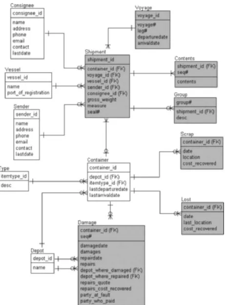
The above query is completely ridiculous but it is the sort of complexity that you might want to search for. The data model for the above query is shown in Figure 2.4.
2.3.2.2 Multiple table joins finding a few fields
Sometimes a join gets at many tables in a data model and only retrieves as little as one field, or even just a few fields, from a single table in a multiple table join. A join could be passing through one or more tables, from which no fields are retrieved. This can be inefficient because every table passed through adds another table to the join. This problem can be resolved in two ways:
By denormalizing tables to fewer tables. However, this may be diffi-cult to implement because so much denormalization could be required, that it may affect functionality in a lot of application code