Random Tournaments

(1)

Random Tournaments

Tejas Iyer

October 2016

(2)

(3)

(4)

(5)

Acknowledgements

I’d like to thank my supervisor Professor Brendan McKay and Dr Mikhail Isaev. Both of them dedicated hours to helping me with this thesis, and without them none of the work would have been possible. I am very grateful for their support.

Thanks also to Associate Professor Scott Morrison for acting as my co-supervisor within the MSI, and providing me with a lot of feedback on earlier drafts. His advice was often very helpful, and I really appreciate the time he spent proofreading.

I’d also like to thank Dr Pierre Portal, who provided me with helpful comments on the final draft of my thesis and Dr Joan Licata for her tireless efforts as Honours coordinator in making the Honours program run as smoothly as possible.

Finally, I’d like to thank my family and friends for all of their support over the years.

(6)

(7)

Introduction

Tournaments are an important class of directed graph. They were first introduced by Landau in 1953 [Lan53] in order to model dominance relations in flocks of chickens and nowadays are used widely in comparison based ranking, with applications to biology, chemistry, networks and sports.

This thesis concerns itself with results related to random tournaments, which are prob-ability distributions over tournaments. In Chapter 1, we provide a brief introduction to the theory of tournaments and prove many famous results in the area. Then, in Chapter 2, we introduce random tournaments and provides a brief survey of results in the field.

In Chapter 3, we introduce the combinatorial objects of multi-tournaments, generalised multi-tournaments and generalised tournaments which are closely related to random tour-naments. By using the tools of convex analysis, we prove some interesting results related to these objects which, for example, have interesting implications for voting theory.

Chapter 4 uses the theory developed in Chapter 3 to derive results related to a special type of random tournament called the β-model. This has many interesting applications to the study of comparison based ranking. By making use of results from this chapter, in Chapter 5 we derive an asymptotic formula for the number of tournaments with a particular score vector (see Definition 1.1.21) that works for a wide range of ‘tame’ score vectors. This provides a means for one to calculate the probability of a tournament with a particular ‘tame’ score vector with respect to any β-model random tournament.

The methodologies in Chapters 3, 4 and 5 are mostly original, inspired by similar results in the field of random graphs and the direction of the author’s supervisor Brendan McKay and Mikhail Isaev. The results are also new, unless otherwise stated.

(12)

(13)

Notation

This thesis will use the following notation:

Notation 0.0.1. Suppose n is a positive integer. We denote by [n] the set {1,2,· · ·, n}. Notation 0.0.2. Letf(x) be a complex valued function andg(x) be a real valued function with both functions taking inputs in _Rn_{. We say} _f_{(x) =}_O₍_g_{(x)) as} _x_{→ ∞} _{if there exists} some positive constant M such that

|<f(x)| ≤M|g(x)|

and

|=f(x)| ≤M|g(x)|,

for |x| sufficiently large.

Notation 0.0.3. Let f(x) and g(x) be real valued functions taking inputs in _R. We say

f(x) = Θ(g(x)) if forx sufficiently large there exist positive constants c1 and c2 such that c1|g(x)| ≤ |f(x)| ≤c2|g(x)|.

Also note that for convenience we will often write vectors inx∈_Rn_{as a list indicating the} components of the vector, so that ifxhas components x1,· · ·, xn, we writex= (x1,· · ·, xn).

(14)

(15)

Chapter 1 Tournaments

In this chapter, we will assume that the reader has some basic familiarity with graph theory.

1.1 Basic Definitions

1.1.1 Preliminaries

Intuitively we may think of a tournament on n vertices as recording the results of a round-robin competition with n players, where each game can only result in a win or a loss. In order to make this precise, we first recall some definitions about directed graphs.

Directed Graphs

Definition 1.1.1. A directed graph, ordigraph D is an ordered pair (V, E), where V is a set of vertices, and E is a set of directed edges consisting of ordered pairs of vertices in V. To avoid confusion between vertex and edge sets of different directed graphs, if D is a directed graph, we use the notationV(D) andE(D) to denote the vertex set of D and edge set of D respectively. In general, we will only consider directed graphs whose vertex set is finite. Moreover, we will assume that there are no loops, that is, edges of the form (v, v). Definition 1.1.2. Two directed graphsD and D0 are said to be vertex disjoint if V(D)∩

V(D0) =∅ and edge disjoint if E(D)∩E(D0) = ∅.

A directed graph may be represented as a diagram where each directed edge (u, v) between vertices u and v is represented as an arrow from u to v. In fact, a lot of the intuition for this subject comes from the pictures, the formalism is just a means for making these ideas rigorous.

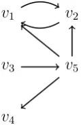
Example 1.1.3. Figure 1.1 is an example of a directed graph on 5 vertices represented as a diagram.

(16)

v1 v2

v3 v5

[image:16.595.275.335.103.195.2]

v4

Figure 1.1: A directed graph on 5 vertices

Definition 1.1.4. LetD be a directed graph. For any vertex v ∈ V(D) the out-degree of

v, denoted deg+(v), is the number of directed edges in E(D) directed from v (i.e edges of the form (v, u), where u ∈ V(D)). The in-degree of v, denoted deg−(v) is the number of directed edges in E(D) directed to v (i.e edges of the form (u, v), where u ∈ V(D)). An isolated vertex v has deg+(v) = deg−(v) = 0.

Example 1.1.5. In Figure 1.1, deg+(v5) = 3 and deg−(v5) = 1.

Often it is useful to consider digraphs contained in larger digraphs.

Definition 1.1.6. Let D be a digraph. A subdigraph D0 of D is a digraph such that

V(D0)⊆V(D) andE(D0)⊆E(D). Given a subsetU ⊆V(D), the subdigraph ofDinduced by U is the subdigraphDU = (U, E(DU)) such that each edge (u, v)∈E(D) with u, v ∈U is contained in E(DU).

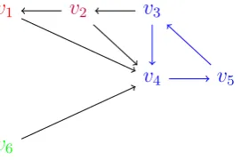
Example 1.1.7. Figure 1.2 shows a digraphD on vertex setV(D) ={v1, v2, v3, v4, v5}, and

the subdigraph DU induced by U ={v2, v3, v5}coloured in red.

v1 v2

v3

v4

v5

Figure 1.2: A subdigraph induced by a set of vertices.

It is also useful to consider directed paths and directed cycles in directed graphs. Definition 1.1.8. A directed trail from vertices v0 to vn in a directed graph D is an alternating sequence v0e1v1e2. . . vn−1envn of vertices vi ∈ V(D) and directed edges ei ∈

E(D), where each ei = (vi, vi+1). Moreover, every edge in the sequence is distinct. The

[image:16.595.256.357.515.602.2]

(17)

1.1. BASIC DEFINITIONS 3 Definition 1.1.9. A Hamiltonian path in a directed graph D is a spanning directed path in it, that is a directed path that hits every vertex inD. AHamiltonian cycle is a spanning directed cycle. A digraph that consists of exactly 1 Hamiltonian cycle is called a cycle digraph or a cycle.

Example 1.1.10. Figure 1.3 below illustrates a directed path (red) and a directed cycle (purple) in a digraph.

v1 v2 v3

v4 v5

[image:17.595.264.409.235.325.2]

v6

Figure 1.3: A directed path in a digraph from vertex v6 to vertex v3 (red), and a directed

cycle (purple).

Definition 1.1.11. Let D be a digraph. If, given vertices u and v in V(D), there is a directed path from u to v, we say that {u → v}. This induces a binary relation on V(D), called the reachability relation. In this case we say v is reachable from u.

A special type of digraph has every vertex reachable from each other:

Definition 1.1.12. A digraph D is called strongly connected or strong if, given any pair of vertices u, v ∈ V(D), {u → v} and {v → u}. A strongly connected component is a subdigraph of D which is strongly connected.

Since a single vertex digraph is strongly connected, evidently the vertices in the strongly connected components of a digraphD partition V(D).

Example 1.1.13. Figure 1.4 shows the digraph of Figure 1.3 partitioned into strongly connected components.

v1 v2 v3

v4 v5

v6

[image:17.595.268.404.653.743.2]

(18)

Oriented Graphs

The main type of directed graph we will encounter in this thesis, is called anoriented graph. Definition 1.1.14. An oriented graph is a directed graph D = (V, E) such that between any pair of vertices u, v ∈V, there can only be one directed edge: (u, v) or (v, u).

The terminology ‘oriented graph’ comes from the fact that these directed graphs may be thought of as graphs where each edge is assigned an orientation, or direction. In particular, given a graph G = (V, E), an orientation of G is a map ψ : E → V ×V, such that each unordered pair of vertices{u, v} ∈Emaps to exactly one of theordered pairs (u, v)∈V×V

or (v, u)∈V ×V. Such an orientation ofGyields a directed graph (V, ψ(E)) in the natural way. Conversely, the condition that there can be exactly one directed edge between any two vertices implies that any oriented graph D is the orientation of some simple graph.

Definition 1.1.15. Given an oriented graph D = (V, E), the underlying simple graph

S(D) is the graph obtained by removing the orientation of each edge. Precisely, S(D) = (V, ψ−1₍_E_{)), where} _ψ−1 _{maps any ordered pair (}_{u, v}₎_∈_E _{to the unordered pair} _{_{u, v}_}_.

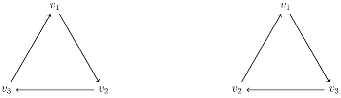
Example 1.1.16. Figure 1.5 shows an oriented graph D on three vertices {v1, v2, v3}, and

the underlying simple graph S(D).

v1 v2 v3

(a) An oriented graph D = (V, E) on three ver-tices. Here V ={v1, v2, v3}and

E ={(v1, v2),(v2, v3)}.

v1 v2 v3

(b) The underlying simple graphS(D)

Figure 1.5: An oriented graph and its underlying simple graph.

We now have the terminology we need to definetournaments.

1.1.2 Tournaments

Definition 1.1.17. A tournament on n vertices is a directed graph obtained by orienting every edge of the complete graph Kn. If, given vertices u and v, an edge is oriented from

u to v, we say that u dominates v. Given u, v ∈ V(T), a game between u and v is the unordered pair {u, v} in the underlying simple graph Kn.

We may thus this of a tournament as the results of the n₂

possible different games between n players, where the result is recorded by orienting the edge.

Example 1.1.18. Figure 1.6 shows a complete graph on five vertices{v1, v2, v3, v4, v5}(left),

(19)

1.1. BASIC DEFINITIONS 5

v1

v2

v3 v4

v5

(a) The complete graphK5

v1

v2

v3 v4

v5

[image:19.595.140.517.88.241.2]

(b) A tournament on 5 vertices.

Figure 1.6: A tournament on 5 vertices obtained by orienting each edge of K5

We denote by _Tn the set of all tournaments on a set of vertices {v1,· · ·, vn}. Such a tournament contains n₂ edges, each of which can be oriented in exactly 2 ways,

|_Tn|= 2(

n

2)_.

Continuing with the analogy of a round-robin competition, the out-degree of the vertex

u then records the total number of wins by u, or the totalscore of u in the competition. Definition 1.1.19. Given a tournamentT, thescore of a vertexv ∈V(T) is the out-degree of v inT.

It is often useful to record the results of each player in a round-robin tournament in a list. This leads us to the following definitions:

Definition 1.1.20. Let T be a tournament on n vertices. An ordering of the vertices of

V(T) is a bijectionπ :V(T)→[n].

Definition 1.1.21. LetT be a tournament onn vertices, with an orderingπ. Ascore vector corresponding toπ is a vectors∈_Rn_{such that each entry}_s

i is the score of the vertexπ−1(i) inT.

If a tournament T has an indexed vertex set {v1, . . . , vn}, we will generally use the term score vector to mean the score vector corresponding to the natural mapπsuch that for each

i∈[n], vi 7→i.

Often it is convenient to arrange the entries in the score vector in non-decreasing order, so that the score vector conveys information about the performance of the players. We give this type of score vector a name:

Definition 1.1.22. A score sequence of a tournament T on n vertices is a score vector s with an ordering such that the entries of the score vector are in non-decreasing order, i.e

(20)

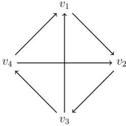
Example 1.1.23. The following tournament on 4 vertices, has score vector s= (2,1,2,1). The score sequence of this tournament is (1,1,2,2).

v1

v2

v3 v4

Figure 1.7

Remark 1.1.24. Note that summing the scores of each of the vertices counts the total number of possible edges between vertices (one may think of this as the total number of games played), so that, for a tournament on n vertices, the sum of the scores will be n₂. This is evident in Example 1.1.23, as we see that that 2 + 1 + 2 + 1 = 6 = 4₂

. Notation 1.1.25. We denote by _T(s) the set of tournaments with score vector s.

If T is a tournament, then any subset U ⊆ V(T) induces a subdigraph which is also a tournament. We call this a subtournament induced by U.

Notation 1.1.26. If U is a subset of V(T) for a tournament T, then we denote byTU the subtournament induced by vertex set U.

Example 1.1.27. Figure 1.8 shows a tournament and a subtournament induced by a vertex set in red.

v1

v2

v3

v4

v5

[image:20.595.243.370.147.298.2]

v6

Figure 1.8: A subtournament of a tournament on 6 vertices induced by the vertex set

{v1, v2, v3, v5}.

Definition 1.1.28. If T is a tournament, and u ∈ V(T), we denote by W(u) the set of vertices in V(T) that are dominated by u, and L(u) the set of vertices that dominate u. Thus, {u},W(u) and L(u) partition V(T).

(21)

1.2. LANDAU’S THEOREM 7

1.2 Landau’s Theorem

An interesting question to ask is which sequences of length n correspond to score sequences of a tournament. Suppose s= (s1, s2,· · ·, sn) is the score sequence of a tournament T. For any subset A ⊆V(T) of sizek let (sA₁,· · ·, sA_k) be the score sequence of the subtournament

TA. We then find that, if Ais the subset of vertices corresponding to the firstk terms of the score sequence,

k

X

i=1 si ≥

k

X

i=1 sA_i =

k

2

.

Thus,

k

X

i=1 si ≥

k

2

for all positive integers k ≤ n, with equality when k = n. In 1953, Landau showed that these conditions are also sufficient [Lan53]:

Theorem 1.2.1 (Landau’s Theorem). A sequence of non-negative integers s1 ≤s2 ≤ · · · ≤ sn is a score sequence for some tournament T ∈Tn if and only if

k

X

i=1 si ≥

k

2

(1.1)

for all positive integers k < n, and

n

X

i=1 si =

n

2

. (1.2)

The following clever proof is due to Carsten Thomassen, from ([Cha81], pages 589-591). We first require the following Definition and Lemma:

Definition 1.2.2. Ifv is a vertex in a tournamentT such that v can reach any other vertex via a path of length 1 or 2,v is called a king.

Lemma 1.2.3. In any tournament T the vertex with the highest score is a king.

Proof. Suppose the vertex with the highest score isv. If u6=v is a vertex such thatu is not reachable from v via a path of length 1, then u dominates v. If u is also not reachable from

v via a path of length 2, then for all vertices w such that v dominates w, it is also the case that u dominates w. This implies that the score of u is strictly larger than the score of v, a contradiction.

(22)

of N.

If there exists M < N such that PM

i=1si = M₂

, the sequence x = (s1,· · ·, sm) satisfies (1.1) and (1.2). Therefore, by the minimality of N, xis the score sequence of a tournament

T1 onM vertices. Moreover,

w

X

i=1

(sM+i−M) = M+w

X

i=M+1

(si−M)≥

M +w

2

−

M

2

−M w =

w

2

for each wsuch that 1 ≤w≤N−M and with equality whenw=N −M. Thus, again by minimality of N, the sequence y = (sM+1 −M, ..., sN −M) is the score sequence of some tournament T2 on N −M vertices. Now, if we form the tournament on N vertices as a

disjoint union of T1 and T2, with edges directed from T2 toT1, then this is a tournament on N vertices with score sequence s, contradicting our assumption.

Now suppose that each inequality in (3.6) is strict when k < N. Then, in particular,s1 >0,

and sN <(N −1). One may easily check that the score sequence (s1−1,· · ·, sN−1, sN + 1) satisfies (1.1) and (1.2), and thus by minimality of s1, has a corresponding tournament.

By Lemma 1.2.3 vN is a king, so there is a directed path of length 1 or 2 from vN to v1.

By reversing the edges of this directed path we obtain a tournament with score sequence (s1,· · ·, sN), a contradiction.

Since any score sequence can be obtained by arranging the scores of a tournament in non-decreasing order, Landau’s Theorem provides conditions for _T(s) to be non empty. In particular, if I ⊆ [n] and s= (s1,· · ·, sn) is any score vector for a tournament T, then the Landau conditions are evidently equivalent to the condition that

X

i∈I

si ≥

_| I|

2

,

with equality if I = [n].

Landau’s Theorem has an interesting application to ranking in sports. Suppose we have a cricket competition consisting of 10 teams, where each team plays against each other once, and every result is either a win or a loss. Suppose the teams are ranked by their number of wins. How many possible winners are there in this competition? The answer is 9, since the sequence of integers (0,5,5,5,5,5,5,5,5,5) satisfies the conditions of Landau’s Theorem (1.1) and (1.2), but no sequence containing ten integers all greater than 4 does.

1.3 Dominance Relations

1.3.1 Relations

(23)

1.3. DOMINANCE RELATIONS 9 orientation of the edge between any pair of vertices.

Many results in the field are related to the problem of ranking vertices based on the structure of a tournament. Under the dominance relation, an unambiguous ‘winner’ of a tournament would be a vertex that dominates every other vertex. This type of vertex has a special name: Definition 1.3.1. If v is a vertex in a tournament T such that v dominates every other vertex, we call v a emperor.

Evidently, a tournament can have exactly one emperor, but it is also the case that many tournaments have no emperors at all. If we weaken the condition on a ‘winner’ v so that v

can reach every vertex via a path of length at most 2, we get the definition of a king of a tournament (Definition 1.2.2). The following Proposition can be proven in a similar way to Lemma 1.2.3.

Proposition 1.3.2 (Adapted from [FH66], Theorem 3). If a tournament T has no emperor, then it contains at least three kings.

Proof. IfT has less that 3 vertices, T always has an emperor. Thus, we may assume T has at least 3 vertices. Letv be a vertex ofT with maximum score. Then by Lemma 1.2.3, v is a king. Also, sinceT has no emperor, there is at least one point which dominatesv. Among all such points, let u be the one with highest score. A similar argument to the proof of Lemma 1.2.3 shows that this is a king. Now, choose a vertexwwith maximum score among those vertices which dominateu. The same argument again shows that this vertex is also a king. Since the dominance relation is asymmetric, and we have that w dominates u and u

dominates v, it follows that these vertices are distinct points, and the result follows.

Examples 1.3.3. Figure 1.9a illustrates an emperor in a tournament, whilst Figure 1.9b shows that Proposition 1.3.2 is tight.

v1

v2

v3 v4

v5

(a) A tournament on 5 vertices with an emperor and its directed edges in purple.

v1

v2

v3

v4 v5

[image:23.595.127.540.572.718.2]

(b) A tournament on 5 vertices with exactly 3 kings (coloured vertices).

(24)

1.4 Directed Paths

A directed path has a natural meaning with regards to tournaments: it represents a sequence of vertices where each vertex dominates the succeeding vertex. The following famous result due to R´edei in 1934 ([R´34]) shows that it is always possible to arrange every vertex in a tournament in such a sequence.

Theorem 1.4.1. Every tournament contains a Hamiltonian path.

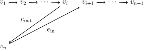
Proof. We use induction on the number of vertices in the tournament. If T denotes a tournament, the base case V(T) = 1 is trivial. If T has n vertices, fix a vertex vn ∈V(T). Then, by induction hypothesis, the subtournament TU induced by the U = V(T)− {vn} has a Hamiltonian path. Suppose this Hamiltonian path is P =v1e1v2· · ·vn−2en−2vn−1. If vn dominates v1 then by adjoining vn to P it is evident that T has a Hamiltonian path. Otherwise, let i be the minimal value of the index such that vn is dominated by vi but dominates vi+1. Then, if eout denotes the edge (vi, vn) and ein denoted the edge (vn, vi+1).

Then the path v1e1v2· · ·vieoutvneinvi+1· · ·vn−1 is a Hamiltonian path inT. v1 v2 · · · vi vi+1 · · · vn−1

vn

eout

[image:24.595.187.456.361.445.2]

ein

Figure 1.10: The above diagram illustrates the inductive step of the proof of Theorem 1.4.1. Example 1.4.2. The following picture illustrates a Hamiltonian path in a tournament on 6 vertices.

v1

v2

v3

v4 v5

v6

v1

v2

v3

v4 v5

v6

Figure 1.11: A tournament on 6 vertices (left), and a Hamiltonian path coloured in red (right).

1.5 Transitive Tournaments

[image:24.595.137.478.529.642.2]

(25)

1.5. TRANSITIVE TOURNAMENTS 11 the tournament may have cycles. However, if the tournament is such that the dominance relation is transitive, it is possible, and such tournaments have a special name:

Definition 1.5.1. A tournament istransitive if its dominance relation is transitive. The following theorem characterises transitive tournaments:

Theorem 1.5.2. The following are equivalent for any tournament T ∈_Tn: 1. T is transitive.

2. The score sequence of T is(0,1,· · ·, n−1). 3. T is acyclic (does not contain a directed cycle). 4. T contains a unique Hamiltonian path.

Proof.

1⇒2 Any transitive tournament must contain an emperor. If this emperor is removed, the resulting tournament is also transitive, and the result follows by induction.

2⇒3 Any emperor cannot be part of a directed cycle, so any such cycle must be part of the subtournament with the emperor removed and again the result follows by induction. 3⇒4 Suppose T is acyclic. If V(T) = 2 the result is clear. If V(T) =n, then the

subtour-nament induced by the vertex set with vn ∈ V(T) removed is also acyclic, and the resulting tournament contains a unique Hamiltonian path. Denote the Hamiltonian path by v1e1v2· · ·vn−2en−2vn−1. Now, reintroduce vn and the incident edges. If vn is an emperor, then the result follows immediately. Otherwise, if there are two indices

i < j such that vi dominates vn which dominates vi+1 (and similarly for vj), then the resulting tournament contains a cycle, as is illustrated in blue in the Figure below.

· · · vi vi+1 · · · vj vj+1 · · ·

vn

Figure 1.12

It follows that there is exactly one index i satisfying this property, and moreover, vn dominates every vertexvj with j > i and j ≤n−1.

4⇒1 Applying a similar argument to the previous proof, if T contains a Hamiltonian path, denoted byv1e1v2· · ·vn−1en−1vn, if eachvi does not dominate every succeeding vertex

(26)

1.6 Irreducible Tournaments and Strong Score Sequences

Another special type of tournament is a reducible tournament:

Definition 1.6.1. A tournament is reducible if it is possible to partition its vertices into sets A and B such that all the vertices in set A dominate all of those in setB. Otherwise a tournament is irreducible.

IfT is a tournament with score sequence (s1, s2,· · ·, sn), evidently T is reducible if and only if for some k < n

k

X

i=1 si =

k

2

.

Therefore, tournament is irreducible if and only if each inequality in (1.1) is strict for

k < n.

Theorem 1.6.2. A tournament is irreducible if and only if it is strong.

Proof. If a tournament T is strong, evidently it must be irreducible. For the converse, suppose T is not strong. Then, for some v ∈ V(T), the set A containing v along with all vertices reachable from v is such that V(T)−A 6= ∅. By partitioning V(T) into A and

V(T)−A, it follows that T is reducible.

Theorem 1.6.3 (Adapted from [FH66], Theorem 7). If a tournament T ∈_Tn is strong, it contains a cycle of length 3,4,· · ·, n. In particular, it contains a Hamiltonian cycle.

Proof. A strong tournamentT ∈_Tnis not transitive, hence must contain a directed triangle. Now, applying induction, suppose T contains a cycle of length k < n, which we denote as

v0e0· · ·vk−1ek−1v0. Suppose for some vertex v outside this cycle, the directed edges (vi, v) and (v, vi+1) are in E(T), where the index values are taken modulo k. Then, by removing

the edge (vi, vi+1) and incorporating these edges, we can form a cycle of lengthk+ 1.

Otherwise, every vertex outside the cycle either dominates, or is dominated by the ver-tices inside the cycle. If we partition the verver-tices outside the cycle into disjoint sets A and

B corresponding to either case, then since T is strong, by Theorem 1.6.2 bothA and B are nonempty. Moreover, there must be a vertex b ∈ B which dominates a vertex a ∈ A. If

ea = (a, v0),eb = (vk−2, b) and ep = (b, a), the cycleaeav0e0· · ·vk−2ebbepais a cycle of length

k+ 1, and this completes the proof.

1.7 Regular Tournaments

(27)

1.7. REGULAR TOURNAMENTS 13 Definition 1.7.1. A regular tournament on n vertices, with n ≥ 3 is a tournament with score sequence

s=

( _n₋₁ 2 ,

n−1 2 ,· · ·,

n−1 2

, if n is odd,

n−2 2 ,

n−2 2 ,· · ·,

n−2 2 ,

n

2,· · ·,

n

2,

n

2

, if n is even. Note that in the case where n is even exactly n₂ vertices have score n−₂2.

Remark 1.7.2. Ifn is even, it is not possible for all of the vertices to have the same score, because this would imply that each vertex has score n−₂1, which is not an integer.

Examples 1.7.3. Here are some examples of regular tournaments on even and odd numbers of vertices.

v1

v2 v3

(a) A regular tournament on 3 vertices

v1

v2

v3 v4

[image:27.595.386.511.304.428.2]

(b) A regular tournament on 4 vertices.

Figure 1.13: Regular tournaments on 3 and 4 vertices.

We see that in the case of 3 vertices, each vertex has score 1, whilst in the case of 4 vertices, v1 and v2 have score 1 and the other vertices have score 2. This shows that the tournaments are regular.

1.7.1 Kelly’s Conjecture

One interesting thing about odd regular tournaments is that it appears that they always can be decomposed into edge disjoint Hamiltonian cycles. This result is known as Kelly’s Conjecture ([KO13]).

Conjecture 1.7.4. Any regular tournament on an odd number of vertices can be expressed as the edge disjoint union of Hamiltonian cycles.

This result, while easy to state, appears to be very difficult to prove. Recently, in 2013, a partial result was obtained by K¨uhn and Osthus, who proved the result to be true when the number of vertices in the tournament is sufficiently large [KO13].

(28)

Example 1.7.6. Figure 1.14 shows an example of a decomposition implied by Kelly’s Con-jecture:

v1

v2

v3 v4

[image:28.595.246.367.174.289.2]

v5

Figure 1.14: A decomposition of a tournament on 5 vertices into edge disjoint Hamiltonian cycles (blue and red).

K¨uhn and Osthus also proved that when n is even a tournament on n vertices has a decomposition into edge disjoint Hamiltonian paths [KO13].

1.7.2 Excess Sequences

We will show in Chapter 2, that in some sense ‘most’ tournaments are ‘close’ to regular (see Theorem 2.4.7). In order to quantify how ‘close’ a tournament is to regular we need excesses.

Definition 1.7.7. Let T be a tournament on n vertices with vertex set V. The excess of a vertex v ∈V(T) is the out-degree minus the in-degree of v inT.

We can then defineexcess vectors andexcess sequences in a similar way to score vectors and score sequences. Often we will use the symbol δ = (δ1,· · ·, δn) to represent an excess vector.

Example 1.7.8. If T is a regular tournament, the excess sequence of T is such that

δ =

(

(0,· · ·,0), if n is odd, (−1,· · ·,−1,1,· · ·,1), if n is even.

In some sense, kδk∞ gives an indication of how close the tournament is to regular. If

kδk∞ is large, then at least one vertex has a much larger out-degree than in-degree or much

larger in-degree than out-degree, and at leastkδk∞−1 directed edges need to be reversed to

get a regular tournament.

(29)

1.8. FURTHER REFERENCES 15

v1

v2

v3 v4

Remark 1.7.10. Note that summing the scores of the vertices and summing the in-degrees both count the number of possible edges between vertices. Thus, if we have an excess sequence δ = (δ1,· · ·, δn) of a tournamentT

n

X

i=1 δi =

X

v∈V(T)

deg+(v)− X

v∈V(T)

deg−(v) =

n

2

−

n

2

= 0.

This is in evident Example 1.7.9 where the sum of the excesses is 3−1−1−1 = 0. We will denote by _Td(δ) the set of all tournaments with excess sequence δ.

1.8 Further References

(30)

(31)

Chapter 2 Random Tournaments

2.1 Introduction

The purpose of this chapter is to give an introduction to the topic ofrandom tournaments. We will then provide a brief survey of the area. Most of the more technical proofs will be omitted, since the approaches tend to vary widely, and are not immediately relevant to the approach taken in this thesis. Results related to paired comparison models and asymptotic enumeration will be considered separately in Chapters 4 and 5. In this chapter, we content ourselves with an overview of the other main results in the field, to provide the reader a broader understanding of the area, and a context for the results proved in Chapters 3 - 5.

We will assume the reader is familiar with basic probability theory. The content of ([Fel68]) should suffice.

2.2 Preliminaries

We define a random tournament in a similar way to the way a random graph is defined ([Bol01], page xiii):

Definition 2.2.1. Arandom tournament Tnonnvertices is a probability distribution over

Tn. We will use the notation T ∈ Tn to denote a tournament valued random variable T drawn from this distribution.

As this is a probability distribution over a finite set, we can generate a random tournament by specifying the probability P(T) of each tournament T ∈ _Tn, so that the sum over all probabilities is 1.

Examples 2.2.2.

1. Theuniform random tournament Un is the uniform distribution over all tournaments defined on a set of n vertices. Each tournament has probability 1

2( n₂₎.

(32)

2. Given a tournament T, the Dirac random tournament on T gives the probability

P(T) = 1, and all other tournaments probability 0.

A more general random tournament may be generated by having each directed edge occur independently of the others, and with a specified probability:

Definition 2.2.3. Theedge model random tournament is the random tournament obtained by having each directed edge from vertex vi to vertex vj occur independently of the others, with specified probability pij.

Clearly we must have pij +pji = 1, since one of the directed edges must occur. We may think of an edge model random tournament as a type of generalised tournament, which will be defined and studied in Chapter 3.

Examples 2.2.4.

1. The uniform random tournament is an edge model random tournament where the directed edge from any vertex vi to any other vertexvj occurs with probability 1₂. 2. The Dirac random tournament is such that, ifpij is the probability of an edge directed

from vertex vi to vj, withi6=j,

pij =

(

1, (vi, vj)∈T, 0, otherwise.

3. Theβ-model random tournament onn vertices, givenstrength parameters β1,· · ·, βn has each directed edge from vertexvi to vertexvj, withi6=j, occurring with probability

pij =

eβi eβi +eβj.

We will discuss this model in depth in Chapter 4. It is used widely in the method of paired comparisons in statistics, under the name Bradley-Terry model.

We can define expected scores of vertices in a random tournament T as follows:

Definition 2.2.5. The expected score si of a vertex vi in a random tournament Tn on n vertices is the expected value of the score of a tournament T ∈ Tn. The expected score vector of a random tournament Tn is the vector ssuch that the ith component of s is si. The expected score sequence of Tn is the sequence obtained by arranging the components of the expected score vector in non-decreasing order.

If pij denotes the probability of a directed edge from vertices vi to vj in a tournament

T ∈Tn, then by linearity of expectation, we have

si =

X

j6=i

(33)

2.2. PRELIMINARIES 19 The results of interest in this chapter are related to the properties a tournament T ∈Tn is ‘expected’ to have, or those properties that occur with ‘large’ probability. Often the probability of a tournament T ∈Tn having a particular property P tends to 1 as n goes to infinity. The convention in a lot of literature related to random graphs is to say that property

P occurs almost surely ([Bol01], pages xiii), but as this is a slight abuse of terminology, we use a different expression:

Definition 2.2.6. Let P be a property of a tournament T ∈ Tn. We say T has property

P asymptotically almost surely (a.a.s.) if the probability of P tends to 1 as n tends to infinity. Equivalently, we may say asymptotically almost all (a. almost all) tournaments

T ∈Tn have propertyP. If the random tournament is the uniform random tournament Un, we will omit Un, and simply say that a. almost all tournaments have property P.

Remark 2.2.7. Another term often used in discrete mathematics and computer science that means exactly the same thing is with high probability (w.h.p.).

Examples 2.2.8.

1. Let Tn be the uniform random tournament, and fix a tournament K. Then a. almost surely, a tournamentT ∈T is not equal to K, since

P(T =K) = 1 2(n2)

=O2−n(n−2 1)

.

2. LetW denote the event that a tournamentT ∈T has a vertexv that dominates every other vertex. ThenW does not occur a.a.s, since

P(W) = n

2n−1 =O 2

−cn

for a constant c >0.

2.2.1 A Note on the ‘Probabilistic Method’

One of the most important, and most beautiful, contributions of the theory of random tournaments is the birth of the probabilistic method. The probabilistic method is a non-constructive proof technique used widely in combinatorics, number theory and other areas. This technique is attributed to Szele, who, in 1943 [Sze43], used it to prove that there are tournaments which contain a large number of Hamilton paths.

Theorem 2.2.9 (Szele, 1943). Let H(T) denote the number of Hamiltonian paths in a tournament T on n vertices. Then there exists T such that

H(T)≥ n!

(34)

Proof. Let Un denote the uniform random tournament. In any Hamiltonian path in a tour-nament X ∈ Un, each of the n−1 directed edges in the path occurs with probability 1₂. Thus, the probability of a particular path is ₂n−11. As there aren! possible Hamiltonian paths (corresponding to the n! arrangements of the vertices), by linearity of expectation

EH(X) = n!

2n−1.

But as

EH(X) =

X

K∈_Tn

P(K)H(K)≤ max K∈_Tn

H(K),

it follows that some tournament T has H(T)≥ n! 2n−1.

In this way, the probabilistic method can be used to convert results about random tour-naments into existence results for tourtour-naments. For more about the probabilistic method, the author strongly recommends reading [?].

2.3 The Regular Random Tournament

In 1974, in [Spe74], Joel Spencer proved a number of results related to the properties a ‘random’ regular tournament is likely to have. The motivation behind this paper has been to develop an approach to attack problems specifically related to regular tournaments, for example Kelly’s Conjecture (Conjecture 1.7.4).

To make this more precise, we define the regular random tournament to be the proba-bility distribution which is uniform on all regular tournaments and zero otherwise. Let RTn denote the set of regular tournaments on a set of n vertices{v1,· · ·, vn}.

Definition 2.3.1. The regular random tournament Rn is the random tournament on n vertices such that, if T ∈Rn then

P(T) =

(

0, T /∈RTn,

1

|RTn|, otherwise.

Remark 2.3.2. We will find an explicit asymptotic formula for |RTn| in Chapter 5.

The following Theorem provides upper and lower bounds for the probability that the set of games played by vertices in a subset (with each score equal to a fixed value m) is a particular set. For T ∈ Rn let Sm be the set of all subsets A such that the score of each

vi ∈A inT is exactly m. Also given such a set A, denote by GA the set of games played by vertices in A, and set

(35)

2.4. THE UNIFORM RANDOM TOURNAMENT 21 Theorem 2.3.3 (Spencer, 1974 [Spe74]). Suppose |A|= k, with k ≤ n0.6 _and _g

1 ∈ S(A).

Then for sufficiently small ε >0 and n sufficiently large,

|S(A)|−1e−k

2 2−ε ≤P

Rn(GA=g1|T ∈RTn)≤ |S(A)|

−1 ek

2 2−ε.

The next Theorem, which is similar to the first, provides upper and lower bounds on the probability that the subtournament induced by a vertex set A, where each vertex has the same score m, is a particular tournament. WithA as defined previously, denote by _TA the set of all tournaments on vertex set A.

Theorem 2.3.4 (Spencer, 1974 [Spe74]). With A as defined previously, suppose |A|= k, with k ≤n0.6_{. Let} _T

1 ∈TA. Then for sufficiently small ε >0 and n sufficiently large

|_TA|

−1

e−(2+ε)k

3

n ≤P

Rn(TA=T1|T ∈RTn)≤ |TA|

−1

e(2+ε)k

3

n,

where TA is the subtournament induced by A.

Spencer also proved the following:

Theorem 2.3.5 (Spencer, 1974 [Spe74]). Set t= [3 log₂n].Then, for a. almost all T ∈Tn, there do not exist subsetsA, B ⊆ {v1,· · ·, vn} with A∩B =∅, |A|=|B|=t such that all of the vertices in A dominates all of those in B (or vice-versa).

In some sense this result makes precise how ‘competitive’ a regular tournament is likely to be: for n large it is very unlikely that that you can split a regular tournament into disjoint subsets of size 3 log₂n such that the vertices of one set dominate the other.

2.4 The Uniform Random Tournament

More generally, results related to the uniform random tournament allow one to make con-clusions about the properties any ‘random’ tournament is likely to have. Thus, a number of results in the literature on random tournaments concern the uniform random tournament. In this section, we provide an overview of the area.

2.4.1 Subgraph Counts

(36)

Example 2.4.1. If the tournament in Figure 3.5 was drawn fromU4, it would contain two

copies of the directed cycle in Figure 3.3 (coloured).

v1

v2 v3

(a) A directed triangle

v1

v2

v3 v4

[image:36.595.109.510.155.293.2]

(b) A regular tournament on 4 vertices.

Figure 2.1: The tournament on the right contains two copies of the directed cycle on the left. One triangle is coloured in teal and the other in purple, with the edge common to both coloured in blue (the edge (v2, v3)).

Evidently, since a tournament is an oriented graph, it can only contain copies of oriented graphs. In this subsection we review some general results related to subdigraphs in a uniform random tournament.

Three Cycles and Four Cycles

Denote by N C3(T) and N C4(T) the number of labeled directed 3 and 4 cycles respectively

in a tournament T. For example, if T1 is the tournament defined by Figure 3.5, then

N C3(T1) = 2. If we have a uniform random tournament T ∈ Un, then given three vertices

v1, v2, v3, the probability of a cycle containing these three vertices is 1₄. Indeed, there are

2 different cycles containing these vertices (illustrated below), and each of these cycles has probability 1₈.

v1

v2 v3

v1

[image:36.595.132.478.571.671.2]

v3 v2

Figure 2.2: The two possible cycles on vertex set {v1, v2, v3}.

By linearity of expectation, ifT ∈Un it follows that

EN C3(T) =

1 4

n

3

(37)

2.4. THE UNIFORM RANDOM TOURNAMENT 23 Similarly,

EN C4(T) =

3 8

n

4

.

A result by (Moran, 1947 [Mor47]) shows that the distribution of both of these are asymptotically normal.

Theorem 2.4.2 (Moran, 1947 [Mor47]). Let T ∈ Un. Then, as n tends to infinity, the distributions of

N C3(T)− 1 4

n

3

q 3 16

n

3

,

and

N C4(T)− 3 8

n

4

q 3 64

n

4

(4n−11)

,

converge to the standard normal distribution.

2.4.2 Hamiltonian Cycles

Recall that a Hamiltonian Cycle in a directed graph is a spanning cycle. Let H(T) denote the number of Hamiltonian cycles in a tournamentT. Then, a similar argument to the case of finding_EN C3(T) shows that

EH(T) = (n−1)!

2n .

In 1995, Svante Janson [Jan95] showed thatH(T) is also asymptotically normally distributed: Theorem 2.4.3 (Janson, 1995 [Jan95]). Let T ∈Un. Then as

VarH(T) =

2

n +O(n

−2

)

(_EH(T))2,

and as n → ∞

H(T)−_EH(T)

p

VarH(T)

converges in distribution to the standard normal distribution.

(38)

Paths of Length Two

Letrij denote the number of directed paths of length 2 from verticesvi tovj in a tournament

T ∈Un. Let Rλ denote the expected number of ordered pairs of distinct vertices vi and vj such that

rij −

n−2 4 > λ.

The following theorem comes from J W Moon ([Moo68], page 42-43):

Theorem 2.4.4 (Moon, 1968 [Moo68]). If w(n) is such that log(n−2) +w(n) → ∞ and

w(n)n−13 as n → ∞, and

λ =

3

4(n−2) (logn−2 +w(n))

1₂ ,

then asymptotically,

Rλ ∼(2π(logn−2 +w(n)))

−1

2 _e−2w(n)_.

Tournaments with a Given Excess Sequence

If we know that a tournament drawn from U has a given score vectorδ = (δ1,· · ·, δn), what is the probability that it contains a copy of a specified oriented graph D? In an enumera-tive result by Gao, Mckay and Wang in 1998 [GMW00], under certain circumstances, the asymptotic probability has been computed.

Let deg_iS(G) denote the degree of vertex vi in the underlying simple graph S(D). More-over, defineδi(D) to be the outdegree of vertexvi inDminus the indegree, and fix an excess sequence δ = (δ1,· · ·, δn).

Also, given an oriented graph Dand an excess sequence δ = (δ1,· · ·, δn), set

β1 =

1 2n

X

1≤j≤n

2δjδj(D)−δj2(D)

+ 1 3n3

X

1≤j≤n

δ_j3δj(D) + 1

n4 X

1≤j≤n

δ_j2 X 1≤j≤n

δjδj(D),

and

β2 =−

1 2n2

X

(j,k)∈D

(δj−δk−δj(D) +δk(D))

2 .

(39)

2.4. THE UNIFORM RANDOM TOURNAMENT 25 Theorem 2.4.5 (Gao, McKay, Wang, 1998 [GMW00]). Let D be an oriented graph con-taining m directed edges such that for each i∈[n], deg_iS(D) = On−12−ε

0

where ε0 is any positive constant. Moreover, let δ = (δ1,· · ·, δn) be an excess vector with each δi =o

n23

, and such that δidegjS(D) = o(n) for all i, j ∈ [n]. Then, for T ∈ Un and β1 and β2 as

defined above

P (D⊆T|δ)∼2−mexpm

n +β1+β2

uniformly as n → ∞.

2.4.3 Discrepancy Results

In the previous subsection we reviewed a number of results regarding random tournaments containing oriented graphs. Informally, many of these results related to drawing a fixed oriented graph on the vertex set of a tournament so that the edges overlapped. In this subsection we review results of a similar flavour: regarding discrepancy.

IfT1 andT2 are tournaments defined on sets ofn vertices, roughly speaking, thediscrepancy

betweenT1 and T2 measures how much their edges can be made to overlap if T1 is drawn on

the vertex set V(T2). More precisely, the positive discrepancy of these tournaments T1 and T2 is defined by

disc+(T1, T2) := max

φ |E(φ(T1))∩E(T2)| − 1 2

n

2

and thenegative discrepancy is defined by disc−(T1, T2) :=

1 2

n

2

−min

φ |E(φ(T1))∩E(T2)|

where the maximum and minimum are taken over all bijections φ from the vertex set of T1

to the vertex set of T2. The reason for the 1₂ n₂ term in these definitions is that any two tournaments can be drawn on the same vertex set so that at least 1

2

n

2

edges overlap.

Indeed, if T1 is drawn randomly on the same set of vertices as T2, then the probability

of a particular edge between a pair of vertices vi and vj overlapping is 1₂. By linearity of expectation, the expected number of common edges is 1₂ n₂, so that there exists at least one drawing of T1 on the vertex set of T2 satisfying the required property.

The (unsigned) discrepancy is defined as

disc (T1, T2) = max{disc+(T1, T2),disc

−

(40)

Let T Rn denote any transitive tournament on n vertices. Then, in ([Spe71], 1971), and ([Spe80], 1980), Spencer showed that a. almost all tournaments T ∈Un are such that

disc+(T, T Rn) = Θ

n32

.

The upper bound in this result was sharpened by Vega in 1983, who showed that a. almost surely

disc+(T, T Rn)≤1.73n 3 2.

In 2015, Bollab´as and Scott [BS15] considered the (unsigned) discrepancy between two tour-naments drawn from Un. They showed that ifT1, T2 ∈Un, then a. almost surely

disc (T1, T2) = Θ

n32plogn

.

This provided an asymptotic answer to the question “how much more can two random tournaments be made to agree or disagree?”

2.4.4 A Surprising Correlation

Let Un be the uniform random tournament on vertices V ={v1,· · ·, vn}. Let a, s and b be three vertices in V, and denote by{a→s} the event that there is a directed path fromato

s, and similarly define{s→b}.

Recall that two events X1 and X2 are said to be negatively correlated if

P(X1∧X2)< P(X1)P(X2),

and positively correlated if

P(X1∧X2)> P(X1)P(X2).

One might expect the events {a → s} and {s → b} to be negatively correlated. Indeed, increasing the probability of the event{a→s}might involve increasing the number of edges directed towards s which might decrease the probability of the event {s → b}. However, a result by Sven Erick Alm and Svante Linussen in 2009 [EL09] shows that, somewhat counter-intuitively this is not the case if the number of vertices n ≥4:

Theorem 2.4.6 (Alm and Linussen, 2009 [EL09]). Let Un be the uniform random tourna-ment on n vertices, with n ≥ 3 , and the events {a → s} and {s → b} as defined above. Then, these two events are negatively correlated ifn= 3, independent ifn = 4, and positively correlated otherwise.

(41)

2.4. THE UNIFORM RANDOM TOURNAMENT 27

2.4.5 Dominating Sets of Vertices

Since the universal random tournament can be expressed as an edge model random tourna-ment with each edge having probability 1₂, one might expect any tournament drawn from this distribution to be ‘competitive’ in the sense that few vertices dominate a large number of other vertices. This is indeed the case.

In 1962, Moon and Moser showed that a. almost all tournamentsT ∈Un are irreducible. In fact, they showed ([Moo62], [Moo68] pages 3-5) that ifI denotes the event that a tournament

T ∈Un is irreducible, then

P(I)− n

2n−2 < 1 2 n

2n−2 2

.

More generally, if δ denotes the excess sequence of a tournament T, a. almost all tour-naments T are such that δ ≤ On12+ε

for any ε > 0. This result has been alluded to in [Spe74], but does not appear to have been explicitly proven, hence we provide a proof here. Theorem 2.4.7. Suppose δ = (δ1,· · ·, δn) is the excess sequence of a tournament T ∈Un. Then, a. almost surely, kδk∞≤O

n12+ε

.

Proof. In Un, we may think of the score of any vertexvi as the sum of n−1 i.i.d Bernoulli random variables, with success probability 1₂. Now, for any vertex vi and constant c > 0, the probability that

P

|δi|> cn 1 2+ε

) = P

|2si−n−1|> cn 1 2+ε

.

By Hoeffding’s inequality applied to si, since Esi = n−₂1, we have

P

si−

n−1 2 > c 2n 1 2+ε

≤2 exp−c

2n ε_,

so that the probability of any vertex having excess larger thatcn12+ε is bounded above by 2nexp−c

2ε

which tends to 0 as n goes to ∞.

Unbeaten k-sets

If a set A⊆V is such that|A|=k, and at least one vertex in Adominates a vertex outside

A, Ais said to be an unbeaten k-set . In (Barbour et al. 1993 [BGQ97]), Barbour, Godbole and Qian have managed to show that the number ofk−setsin a random tournamentT ∈Un is well approximated (with respect to a probability metric) by a Poisson Distribution with mean

n k

(42)

2.4.6 Quasi-Random Results

A class of properties of tournaments is said to be quasi-random if T ∈Un (or any random tournament Tn) satisfies one of them, then a.a.s T satisfies all of them. These properties are particularly significant in relation to the uniform random tournament because it means that if n is large, then in order to verify that a tournament T satisfies a variety of properties, with a high probability it is enough to verify that one property holds.

A quasi-random class of properties have been studied in a paper by Fan Chung and Ronald Graham [Chu91]. In order to state their result we will need to introduce some terminology.

Suppose T is a tournament on vertex set V with |V|= n. Let

T T0

denote the number of copies of a digraph T0 inT.

For u, v ∈V, we denote by

same(u, v) :=|(W(u)∩W(v))∪(L(u)∩L(v))|.

Intuitively, this denotes the set of vertices w whose encounter with u and v is the same (ie

w dominates u and w dominates v orw is dominated by u and w is dominated by v).

Finally, if T has excess vector δ = (δ1, ..., δn), we say T isalmost balanced if n

X

i=1

|δi|=o(n2).

We are now able to state the main result of (Chung and Graham, 1991 [Chu91]):

Theorem 2.4.8 (Chung and Graham, 1991 [Chu91]). Let Un be the uniform random tour-nament on vertex set V, and let T ∈ Un. The following form a quasi-random class of properties of T:

1. If T0 is a tournament on s vertices, s≤n

T T0

= (1 +o(1))ns2−(s2).

2. N C4(T) = (1 +o(1)) n

4

2 .

3. P

u,v∈V

same (u, v)− n₂

=o(n3).

4. P

u,v∈V

|W(u)∩W(v)| − n₄

=o(n3).

5. For all subsets X ⊂V, the subtournament TX is almost-balanced. 6. Every subtournament of T on bn

(43)

2.5. THEP MODEL RANDOM TOURNAMENT 29 7. For every partition ofV =A∪B with |A|=bn

2c and |B|=d

n

2e, we have X

v∈A

||W(v)∩B|−|L(v)∩B||=o(n2).

8. For all A, B ⊂V,

X

v∈A

||W(v)∩B| − |L(v)∩B||=o(n2).

9. For every ordering π of T,

|{(u, v)∈E(T) :π(u)< π(v)}|= (1 +o(1))n

2

4 .

2.5 The

p

Model Random Tournament

A few results have been proved for a more general type of random tournament, which we call thep-model random tournament.

Definition 2.5.1. The p-model random tournament Tn(p) on the ordered vertex set [n] is a type of edge model random tournament where the probability of a directed edge from vertex i to vertexj isp if i < j, and 1−p otherwise.

To the author’s knowledge, this type of random tournament was first studied by (Frank, 1968 [Fra68]), who showed that for T ∈Tn(p),

EN C3(T) =

n

3

p(1−p) and

VarN C3(T) =

n

3

p(1−p)

1−p(1−p) + n−3 2

.

Note that this is consistent with the casep= 1₂ in (2.4.1).

In 1996, (Luczaks et al. [RG96]) proved a number of asymptotic results related to this random tournament, when p can vary as a function of n.

For a graph G= (V(G), E(G)), define d(G) to be the ratio

d(G) = |E(G)|

|V(G)|,

(44)

Theorem 2.5.2 (Luczacs et al. 1996 [RG96]). Let T ∈Tn(p) and letD be a oriented graph with at least one cycle. Then,

lim

n→∞P(D⊆T) =



  

  

0, if npm(S(D)) _→₀_,

1, if n(min{p,1−p})m(S(D)) → ∞,

0, if n(1−p)m(S(D)) →0.

Now, if T ∈Tn(p), define

α := min{i: (i, j)∈T for some j > i},

and

β:= max{j : (i, j)∈T for some i < j}.

In the same paper, (Luczacs et al.) showed the following:

Theorem 2.5.3 (Luczacs et al. 1996 [RG96]). Let T ∈Tn(p). If n2p→ ∞ and p ≤ 1₂, a. almost surely the set {α, α+ 1,· · ·, β} is the vertex set of a strong component of T.

Note that this result can be extended to random tournaments withp≥ 1

2 by the duality

(45)

Chapter 3 More General Types of Tournament

3.1 Introduction and Literature

In this chapter we will briefly describe some more general types of tournaments. There are three types of classes we will consider: generalised tournaments, multi-tournaments and generalised multi-tournaments.

It is difficult to find literature on these more general classes of tournaments. The class of generalised tournaments was, to the best of our knowledge, first introduced by Moon [Moo63]. In [Jec83], Jech introduced the types of tournament we will call generalised multi-tournaments, motivated by applications to comparison based ranking.

The primary motivation behind this chapter is to study these types of tournaments in the context of polytopes. As a result much of this chapter will assume basic knowledge of con-vex analysis, which may be found in any introductory text on on the subject (for example [HU01]). As generalised tournaments are closely related to random tournaments, the results proved in this chapter will be useful in Chapters 4 and 5. On the way we provide proofs of some Landau-like theorems for these types of tournaments. In particular, Theorem 3.3.12 shows that for any score vector s there exists a generalised tournament with this score vector that can be expressed as the convex combination of transitive tournaments. We will explain this more detail later on, but this has an interesting interpretation in terms of voting theory (Subsection 3.3.4).

3.1.1 A Word on Notation and Terminology

In this chapter we will use terminology and notation related to convex analysis. We will assume the reader has some familiarity with these terms.

Given a set S ⊆ _Rn _{recall that the} _{affine hull} _of _S _{is the set of affine combinations of} vectors in S.

(46)

Notation 3.1.1 (Affine Hull). We denote by aff(S) the affine hull of S.

Also recall that convex hull of a set is defined similarly, in terms of convex combinations rather than affine combinations.

We use the standard notation for open balls:

Notation 3.1.2 (Ball). Given a point p ∈ _Rn _and _r _∈

R+, we denote by Br(p) the open ball of radius r centred at p.

Finally, recall that the relative interior of a set in _Rn _{is the interior of the set when} viewed as a subset of its affine hull. Specifically, the relative interior of a set S ∈_Rn _{is the} set

{x∈S :∃ε >0 such that Bε(x)∩aff(S)⊆S} We then have the following notation:

Notation 3.1.3 (Relative Interior). Given a set S ∈_Rn_{, we denote by rint (}_S_{) the} _relative interior of S.

3.2 Multi-Tournaments

A tournament can be thought of as encoding the results of a round-robin competition, where every pair of individuals competes against each other once. A multi-tournament allows the possibility of multiple encounters, as is the case with many sporting leagues around the world. Let M be an n×n symmetric matrix with each entry mij ∈Z, and

mij

(

= 0, i=j,

>0, i6=j. (3.1)

Definition 3.2.1. A multi-tournament T on a labelled vertex set V = {v1,· · ·, vn} with schedule matrix M is an orientation of the multi-graph on the vertex setV havingmij edges between vertices vi and vj.

Remark 3.2.2. A multi-tournament is hence a type of multidigraph, or a quiver. Example 3.2.3. Figure 3.1b is an example of a multi-tournament with schedule matrix

M =



   

0 2 1 3 2 0 1 1 1 1 0 1 3 1 1 0



(47)

3.2. MULTI-TOURNAMENTS 33

v1

v2

v3 v4

(a) A multi-graph corresponding to the schedule matrixM.

v1

v2

v3 v4

(b) A multi-tournament with schedule matrix M.

Figure 3.1

We define the score of each vertex, the score vector, and score sequence in a similar way to usual tournaments so that, ifsis the score sequence of a multi-tournament, then the following Landau-like conditions are satisfied:

k

X

i=1 si ≥

X

i<j, i,j∈[k]

mij, (3.2)

for each k ∈[n], with equality if k=n.

Example 3.2.4. The score vector s of the multi-tournament in Figure 3.1b is (4,3,1,1). The score sequence is (1,1,3,4) and one may readily check that conditions (3.2) are satisfied. One may immediately wonder whether these Landau-like conditions are also sufficient. The general case appears to be difficult, but a very similar proof to Theorem 1.2.1 in Chapter 1 shows that there is a Landau-like theorem in the particular case that each mij is equal to some constant p.

Theorem 3.2.5. LetM be the schedule matrix for a multi-tournamentT where eachmij =p for i 6=j. A sequence of non-negative integers s1 ≤ s2 ≤ ...≤ sn is a score sequence for T if and only if

k

X

i=1

si ≥p

k

2

(3.3)

for all positive integers k < n, and n

X

i=1

si =p

n

2

. (3.4)

(48)

3.2.1 Generalised Multi-Tournaments

In generalised multi-tournaments every game between participants i and j results in each player given a rating corresponding to their performance. The sum of the ratings of both players is always 1. For example, if the result was a draw, both players iand j might get 1₂. Definition 3.2.6. A generalised multi-tournamentGwith schedule matrix M onn vertices is an ordered pair (V, T). Here V is a finite set of vertices {v1, ..., vn} and T is a collection of non-negative real number edges {tq_ij :i, j ∈[n], q ∈[mij]} such that tqij +t

q

ji = 1, t q jj = 0 and 0≤tq_ij ≤1. If we setK = 2P

1≤i<j≤nmij +n, we may think of the edge set as a vector t ∈_RK _{obtained by adjoining the edge values.}

Example 3.2.7. We may think of a normal tournament as a generalised multi-tournament, where each tq_ij is either 0 or 1, corresponding to whether i dominates j or

j dominates i.

Definition 3.2.8. Let G = (V, T) be a generalised multi-tournament. Given a vertex

vi ∈V, the score si of vi is the sum n

X

j=1

mij X

q=1 tq_ij.

We then definescore sequences andscore vectors in a similar way to other tournaments. It is possible to prove the following generalisation of Landau’s Theorem for generalised multi-tournaments:

Theorem 3.2.9. Let M be the schedule matrix for a generalised multi-tournament G. A sequence of non-negative real numbers s1 ≤ s2 ≤ ... ≤ sn is a score sequence for G if and only if

k

X

i=1 si ≥

X

i<j, i,j∈[k] mij,

for all positive integers k ≤n, with equality if k =n.

Proof. The proof of necessity of these conditions is straightforward. For ease of notation, we will only prove sufficiency in the specific case where each mij = 1, in Theorem 3.3.12, however the main idea is as follows:

1. Construct polytopes PM (depending on the schedule matrixM) corresponding to the necessary conditions a score vector must satisfy (similar to Definition 3.3.3).

2. Compute the vertices of this polytope using a similar argument to Proposition 3.3.7. 3. Observe that these vertices correspond to the score vector of a specific type of

(49)

3.3. SOME POLYTOPES 35

3.3 Some Polytopes

In this section we outline an approach to study generalised multi-tournaments using poly-topes. For brevity, we only study the particular case of a generalised multi-tournament where each mij = 1 for i6=j, but the results for the other cases are similar.

LetQ be the symmetric n×n matrix such that Qij = 0 ifi=j and 1 otherwise.

Definition 3.3.1. Ageneralised tournament is a generalised multi-tournament with sched-ule matrix Q.

We may think of a generalised tournament as the combinatorial structure underlying an edge model random tournament. This type of tournament G may be represented as a diagram of with directed edges from vertices vi to vj labelled with the value of the edgetij. By convention, we will only draw edges having values greater than or equal to 1₂, and assume any unlabelled directed edge has value 1.

Example 3.3.2. The following diagram illustrates a generalised tournament on 4 vertices:

v1 v2 v3 v4 2 3 1 2 4 5 2 π

Figure 3.2: A generalised tournament on 4 vertices. This tournament has score vector

7 6, 8 15, 9 5 + 2 π, 5 2 − 2 π .

The Landau-like conditions for generalised tournaments imply that the set of ‘permissible’ score vectors of a generalised tournament are those satisying a set of linear inequality and equality constraints. Indeed, if s∈_Rn _{is a score vector then}

1. si ≥0 ∀i∈[n], 2. ∀I ₍[n] P

i∈Isi ≥ |I₂|

, 3. Pn

i=1si = n₂

.

We may thus think of the set of all score vectors of generalised tournaments onn vertices as a convex polytope in _Rn_{. We call this the} _{score vector polytope} _.

Definition 3.3.3. The score vector polytope is the convex polytope defined by:

P_Qn:=

(

s∈_Rn_:_s

i ≥0 ∀i∈[n], ∀I ([n]

X

i∈I

si ≥

_| I| 2 , n X i=1 si =

n

2

)

(50)

Now if G is a generalised tournament on n vertices with score vector s, the edges {tij :

i, j ∈ [n]} that define G are also vectors that satisfy a set of linear equality and inequality constraints and thus also define a convex polytope.

Definition 3.3.4. We call the set

GTn :=

n

t ∈_Rn2

:tjk ≥0, tjj = 0, ∀k6=j tjk+tkj = 1

o

the polytope of generalised tournaments on n vertices . Definition 3.3.5. We call the convex polytope

GTn(s) :=

(

t ∈_Rn2 :tjk ≥0, tjj = 0, ∀k6=j tjk+tkj = 1, n

X

k=1

tjk =sj

)

the polytope of generalised tournaments with score vector s .

Note that by the necessity of the Landau-like conditions, we have GTn=S_s∈Pn

QGTn(s).

We now proceed to work out some details about these polytopes.

3.3.1 Vertices of the Polytopes

In this subsection we find the vertices of some of these polytopes. This is significant, because since these polytopes are bounded, they are equal to the convex hull of their vertices ([Zie95], Theorem 1.1).

Proposition 3.3.6 (Vertices ofGTn). The vertices ofGTn correspond to usual tournaments

T ∈_Tn.

Proof. This proof is rather straightforward, and follows from the definition of vertices of a polytope.

Proposition 3.3.7 (Vertices ofPn

Q). The vertices of PQnare the vectors corresponding to the

n! permutations of (0,1,2,·, n−1). Proof. Suppose s∈Pn

Q has its ith component si =n−1. Then, the conditions on PQnimply that this is the maximum possible value ofsi, so that ifsis the convex combination of vectors in P_Qn, all of these vectors have their ith components equal to n−1. The maximum value of any of the other components of these vectors is then n−2, so that if the jth component of s is n−2, then the jth component of all of these vectors is n−2. By iterating in this manner, it follows that s can only be expressed as the convex combination of itself in Pn Q and therefore must be a vertex.

Suppose that a vector s ∈ Pn

Random Tournaments