Fiscal policy, monetary policy and the transmission mechanism of shocks

Fiscal and Monetary Policy and

the Transmission Mechanism of

Shocks

Jasmine Zheng

October 2013

A thesis submitted for

the

degree of

Doctor

of Philosophy

of

The Australian

National University

Centre

for Applied

Macroeconomic Analysis ( CAMA)

Declaration

I certify that this thesis is my own original work. It contains no material which has been accepted for the award of a degree or diploma in any university and, to the best of my knowledge and belief, contains no material previously published by another person, except where due reference is made in the text of the thesis.

Jasmine Zheng

Preface

• Chapter 2 is based on a paper that is a joint work with-Renee Fry-lVIckibbin. • A version of Chapter 3 is released as Zheng, J. (2013) Effects of US

Nfon-etary Policy Shocks During Financ_ial Crises - A Threshold Vector Autore-gression Approach, Centre for Applied lVIacroeconomic Analysis Working Paper No. 64/2013.

Acknowledgments

As I near the end of my PhD journey at The Australian National

Univer-sity (ANU), I would like to express my gratitude to those who made this thesis

possible. First and foremost, I would like to express my deep and sincere grat

-itude to the Chair of my Supervisory Panel, Professor Renee Fry-l\!Ickibbin for

her supervision, advice and inspiration. I will always remember particular advice she gave me, namely that I should stop reading too much into the literature and

simply start working on what I think is right and that I should always aim to

produce cutting-edge research. I am thankful for the continuous support and

encouragement she has provided me through my studies.

I am also deeply indebted to my other supervisors, Professor Warwick l\!Ick

-ibbin and Associate Professor Ippei Fujiwara. Their comments and suggestions

have helped to improve this thesis and have provided new ideas for future re-search.

I acknowledge the funding support from the Australian Postgraduate Award and ARC Discovery Project DP0985783 during my studies.

I am grateful for the comments received at the Centre for Applied

Macroeco-nomic Analysis lunch time seminar sessions, from colleagues during my internship

at the Reserve Bank of Australia and from discussants and audience members

at the 25th PhD Qonference in Economics and Business (University of Western Australia, 2012) and the Econometric Society Australasian l\!Ieeting (University

of Syd~ey, 2013). I thank Professor John Quiggin for comments on some of the

work included in this thesis.

I would to thank my peers and the academic and administrative staff at the Research School of Economics, Centre of Applied Macroeconomic Analysis

and Crawford School of Public Policy for providing a friendly and supportive environment to work on my research over the last few years. I would also like to

thank my colleagues at the Reserve Bank of Australia for providing an intellectual

working environment for my internship, which has provided me with ideas for

future research.

Thanks also to my ex-colleagues at the Ministry of Trade and Industry in Singapore for the countless interesting conversations that have inspired me to come back to university after four years of work to start on the PhD.

This PhD journey would not have been possible if not for the support from many friends, loved ones and people who have shown care and concern for me along the way. I would like to thank Kastoori, 1\!Iushira, Rachel, Nisal, Varang, Weichen, Cody, Yixiao, Larry and Vittorio for being there for me in Canberra. Thanks also to those in Singapore, Nerine, 1\!Iinghui, Fong Yeng, Angeline, Wen-bing and Ruimin, for the conversations, continuous support and encouragement over the years, most of which have taken place virtually. Thank you for not forgetting me even when I have not been back all that much over the last few years.

Finally, I would like to thank my mom and brother for the unconditional love, support and encouragement given to me throughout my studies. This thesis is dedicated to the never ending pursuit of knowledge.

Abstract

This thesis focuses on the three central themes that have dominated the world economy in recent decades. First, in each of the localized financial crises that has taken place in the world economy, policymakers around the world have re-duced policy interest rates to help stimulate the economy. The recent subprime mortgage crisis and the subsequent Great Recession resulted in the reduction of policy interest rates in many advanced economies to historically low levels. Second, governments around the world have implemented huge fiscal stimulus packages. Third, emerging market economies and countries such as Australia, with close trade linkages to China, have remained resilient. The severity of the crisis of 2007-2011 and the resilience displayed by some economies have resulted in renewed interest among policymakers in investigating the transmission mech-anism channels of economic shocks, fiscal and monetary policies.

There are three main objectives in this thesis. The first Qbjective is to examine the impact of fiscal and monetary policies on the US economy. Chapter 2 uses the Factor Augmented Vector Autoregression (FAVAR) methodology to estimate the impact of fiscal and monetary policy shocks on the US economy. Specifically, the FAVAR model initially used in a monetary policy setting is extended to include a fiscal sector, taking into account of the debt sustainability issue.

The second oq,iective of the thesis is to investigate the asymmetry in the effects of conventional monetary policy on the economy dependent on financial stress ~onditions. A Threshold Vector Autoregression (TVAR) model is used to analyze the effects of monetary policy on the US economy during periods of low and high financial stress, specifying a financial stress index as the threshold variable.

The third objective of the thesis is to study the transmission of economic shocks from the US and Chinese economies to the Australian economy. It is also in the interest of this thesis to analyze if the resilience of the Australian economy in the recent crisis can be partially explained by the increasing trade linkages

Australia has with China. Chapter 4 in this thesis uses a FAVAR approach and a large dataset of 414 macroeconomic variables to analyze the international trans-mission mechanisms between the Australian economy and the US and Chinese

economies.

Overall, this thesis finds evidence suggesting that fiscal and monetary policies can be effective and potent in helping the US economy recover from a financial crisis. Through the analysis of the impact of fiscal and monetary policies on the US economy, this thesis finds that government spending plays an important role compared to other policy levers. The effects of a government spending shock last for a longer period of time and explain more variability in the macroeconomic variables in the US economy, with some crowding-out effects in the medium term. There is also evidence that suggest that fiscal and monetary policies move in opposite directions following a shock to one policy instrument, which weakens the overall impact of an expansionary fiscal or monetary policy. Analyzing the impact of monetary policy on the US economy during periods of low and high financial stress provides further insights. The effects of monetary policy on the US economy are found to be nonlinear. Hence, the impact of monetary policy on the US economy is found to be greater during periods of high financial stress when the size of the shock is larger. There is also evidence of a cost channel effect during periods of high financial stress which points towards a worsening of the short run inflation-output trade off during financial crises.

I

The FAVAR model developed in this thesis to analyze the international trans-mission of economic shocks from the US and China to Australia suggests that the US economy continues to play an important role in the Australian economy, despite the increase in trade linkages between Australia and China. Importantly, there is evidence that economic shocks are transmitted to the Australian econ-omy not solely via the traditional trade and financial transmission mechanisms, but also via the consumer sentiment channel.

List of Acronyn1s

ANFCI Adjusted National Financial Conditions Index CPI Consumer Price Index

DSGE Dynamic Stochastic General Equilibrium EFP External Finance Premium

FAVAR Factor Augmented Vector Autoregression FFR Federal Funds Rate

FRED Federal Reserve Economic Data database GDP Gross Domestic Product

GNE Gross National Expenditure

HQ Hannan-Quinn information criterion Il\JIF International Monetary Fund

IRF Impulse Response Function

LSTVAR Logistic Smooth Transition Vector Autoregression l\JISVAR Markov-switching Vector Autoregression

NIPA National Income and Product Accounts

OECD Organisation for Economic Co-operation and Development OLS Ordinary Least Squares

PPI Producer _J Price Index RBC Real Business Cycle S&L Savings and Loans SC Schwarz Criterion

STVAR Smooth Transition Vector Autoregression SVAR Structural Vector Autoregression

TVAR Threshold Vector Autoregression US The United States ( of America) VAR Vector Autoregression

WTI West Texas Intermediate

Contents

Contents

List of Tables

List of Figures

1 Introduction

1.1 Overview .

1.2 Key Objectives

1.3 fethodological Approaches

1.4 Thesis Outline . . . . . . . .

2 Role of monetary and fiscal policy in explaining US

nomic fluctuations: A FAVAR approach

2.1 Introduction . . . .. . . .

2.2 FAVAR U:odel of fiscal and monetary policy

2.2.1 FAVAR model .

2.2.2 Iden ification of he FAVAR

2.2.3 Identification of the factors .

2.2.4 Estimation .

2.2.5 Data . . .

2. 3 Empilical results

2.3.1 ~ fonetary polic shock

2.3.2 Government expenditure shock

Vlll

Vlll

Xll

XIV

1

1

3

4 6

macroe

co-7

7

11

12

12

16

17

18

19

19

2.3.3 Taxation revenue shock .. 2.3.4 Debt-to-GDP ratio shock .

2.4 Forecast error variance decomposition .

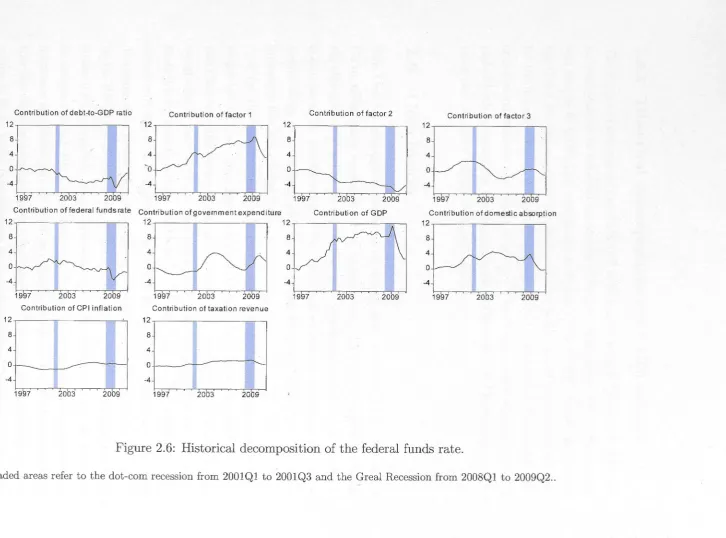
2.5 Historical decompositions . . . 2.5.1

2.5.2

2.5.3

Historical decomposition of S GDP

Historical decomposition of he federal funds ra e Historical decomposi ion of US CPI inflation 2.6 Conclusion . . . .

3 Effects of US monetary policy shocks during financial crises: A 23

25 27

30

31

31

34

34

TVAR approach 37

3.1 Introduc ion . 37

3.2 Background review

3.2.1 redit channels of monetar polic ransID1Ss1on 3.2.2 Cos channel of mone ar policy ransmis ion 3.2.3 Exiting e, 'dence

3.3 Empirical sp cilications . 3.3.1 lvfodel .. ..

3.3.2 Data and specilication is ues . 3.3.3 Tran ition raiiable . . . .

3.4 TI .. AR model estima ion and nonlineari -tes 3.5 Empirical,result . . . . .. . . .. . .

3.5.1 Regime-dependent impulse responses

40

40

42

44 47 47 4

49 49 51 52 3.5.2 Nonlinear impulse re ponses . . . . . 55 3.5.3 Effect of monetary policy hocks in different regimes 56 3.5.3.1 Expansionary monetary policy in different regime 57 3.5.3.'2 Contractionary monetary policy in different regime 59 3.5.4 EfEect of mall ver us large hocks . . .. . .. . .. . . . .. . 61 3 .. 5.4.1 Small veL us large expansionary monetary polic 61 3.5.4.2 Small versus large contractionary monetary policy 62

4

3.5.5 Extension of the sample to 2012Q4

3.5.6 Impact of monetary policy shocks on the probability of

regime switching

3.6 Conclusion . . . .

Transmission of shocks from the US and China to the Australian

economy

4.1 Introduction .

4.2 International transmission mechanism of

shocks

4.2.1 Trade and economic integration transmission

channels

4.2.2 Financial linkage transmission channel

4.3 Empirical methodology .

4.3.1 An Australian economy FAVAR

4.3.2 Identifying the factors

-4.3.3 Identifying the shocks

4.3.4 Data and estimation

4.4 Empirical results

4.4.1 Identified factors

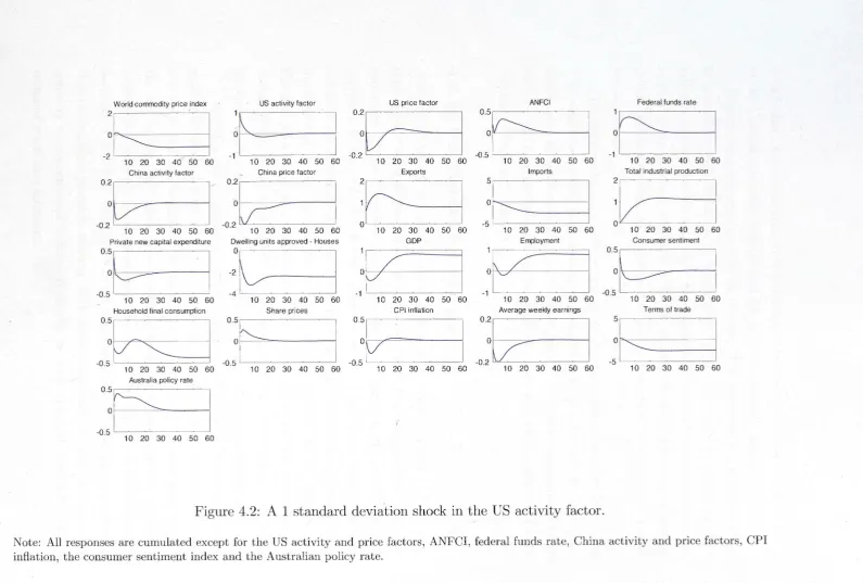
4.4.2 US activity shock

4.4.3 US price shock

4.4.4 US financial conditions shock

. 4.4.5 Federal funds rate shock

4.4.6 Chinese activity shock

4.4.7 Chinese price shock .

4.4.8 Commodity price shock .

4.5 Forecast error variance decomposition .

4.6 Robustness

4.7 Conclusion .

5 Concluding remarks

5.1 Summary .. 5. 2 Main findings 5.3 Policy implications

5.4 Future research directions

A Chapter 2 Appendices

A. l Estimation methodology A.2 The data . . . .

A.3 Additional forecast error variance decompositions

B Chapter 3 Appendices

B.1 Data . . . .

100

100 101 103 104

106

106 107 109

119

119 B.2 Algorithm for computation of nonlinear impulse responses 120 B.3 Confidence bands for nonlinear impulse responses . . . . . 121 B.4 Confidence bands for the impulse responses estimated from sample

1973Ql - 2008Q4 . . . . . . . . . . . . . . . . . 122 B.5 Impulse responses for 1973Ql - 2012Q4 sample 122 B.5.1 Regime-dependent impulse responses 132 B.5.2 Nonlinear impulse responses

C _Chapter 4 Appendices

C.l Estimation of the Australian economy FAVAR C.2" Data set ..

C.3 · Robustness

Bibliography

Xl

132

137 137 139 139

List of Tables

2.1 First criterion: Pure sign restrictions. . . . . . . . . . . 15

2.2 Contribution of shocks to variance of output (percent). 29

3.1 Asymptotic p-values for sup-Wald statistics of non-linearity tests. 51

4.1 Contribution of shocks to Australian macroeconomic variables

(per-cent). . . . . . . . . . . . . . . . . . . . . . . . . . . . 96

A.l Variables used to extract the unobserved US factors. 110

A.2 Forecast error variance decomposition due to the federal funds rate

shock. . . . 115

A.3 Forecast error variance decomposition due to government expen

-diture shock. . . . . . . . . . . . . . . . . . . . . . . . . . . . . . . 116

A.4 Forecast error variance decomposition due to government taxation

revenue shock. . . . . . . . . . . . . . . . . . . . . . . . 11 7

A.5 Forecast error variance decomposition due to debt-to-GDP ratio

shock. . . . . . . . .. . . 118

B. l Data sources.

C.l US variables.

C.2 Chinese variables.

C.3 Australian variables.

C.4 Contribution of shocks to Australian macroeconomic variables

-119

140

144

148

estimation with WTI oil price. . . . . . . . . . . . . . . . . 159

C.5 Contribution of shocks to Australian macroeconomic

variables-estimation without commodity and WTI oil prices. . . 159

List of Figures

2.1 A 1 standard deviation shock in the federal funds rate. 2.2 A 1 standard deviation shock in government expenditure. 2.3 A 1 standard deviation shock in government taxation revenue. 2.4 A 1 standard deviation shock in debt-to-GDP ratio.

2.5 Historical decomposition of GDP.

2.6 Historical decomposition of the federal funds rate. 2.7 Historical decomposition of CPI inflation . .

3.1 The Adjusted National Financial Conditions Index and its esti -mated threshold value.

3.2 Impact of a 1 standard deviation decline in the federal funds rate in the low and high financial stress regimes.

3.3 The effects of a 1 standard deviation decline in the federal funds 22 24 26

28 32

33

35

50

53

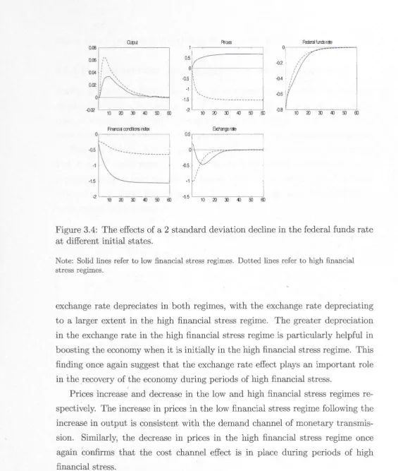
rate at different initial states. . . . . . . . . . . . . . . . . . . . . 57 3.4 The effects of a 2 standard deviation decline in the federal funds

rate at different initial states. . . . . . . . . . . . . . . . . . . . . 58 3.5 The effects of a 1 standard deviation increase in the federal funds

rate at different initial states. . . . . . . . . . .- . . . . . . . . 59 3.6 The effects of a 2 standard deviation increase in the federal funds

rate at different initial states. . . . . . . . . . . . . . . . . . . 60 3. 7 The effects of a 1 and 2 standard deviation decline in the federal

funds rate in the low financial stress regime. 61

3.8 The effects of a 1 and 2 standard deviation decline in the federal

funds rate in the high financial stress regime. . . . . . 62

3.9 The effects of a 1 and 2 standard deviation increase in the federal

funds rate in the low financial stress regime. . . . . . . 63

3.10 The effects of a 1 and 2 standard deviation increase in the federal

funds rate in the high financial stress regime. . . . . . . . . . . . . 64

3.11 Empirical probability of switching from low to high financial stress

regime over time. . . . . . . . . . . . . . . . . . . . 67

3.12 Empirical probability of switching from high to low financial stress

regime over time. . . . . . . . . . 68

4.1 Identified US and Chinese factors 82

4.2 A 1 standard deviation shock in the US activity factor. 84

4.3 A 1 standard deviation shock in the US price factor. . 86

4.4 A 1 standard deviation shock in the ANFCI. . . . . . 88

4. 5 A 1 standard deviation shock in the federal funds rate. 90

4.6 A 1 standard deviation shock in the Chinese activity factor. 92

4. 7 A 1 standard deviation shock in the Chinese price factor. . . 94

4.8 A 1 standard deviation shock in the world commodity price. 95

B. l 68 percent confidence bands for a 1 standard deviation decline in

the federal funds rate with fixed regimes. . . . . . . . . . . . 123

B. 2 68 percent confidence bands for a 1 standard deviation decline in

the federal funds rate at different initial states. . . . . . . . . . . . 124

B.3 68 percent confidence bands for a 2 standard deviation decline in

the federal funds rate at different initial states. . . .. . . . . . . . . 125

B.4 68 percent confidence bands for a 1 standard deviation increase in

the federal funds rate at different initial states. . . . . . . . . 126

B.5 68 percent confidence bands for a 2 standard deviation increase in

the federal funds rate at different initial states. . . . . . . . 127

B.6 68 percent confidence bands for a 1 and 2 standard deviation

decline in the federal funds rate in the low financial stress regime. 128

B. 7 68 percent confidence bands for a 1 and 2 standard deviation

decline in the federal funds rate in the high financial stress regime. 129

B.8 68 percent confidence bands for a 1 and 2 standard deviation

in-crease in the federal funds rate in the low financial stress regime. . 130

B.9 68 percent confidence bands for a 1 and 2 standard deviation in

-crease in the federal funds rate in the high financial stress regime. 131

B.10 Impact of a 1 standard deviation decline in the federal funds rate

in the low and high financial stress regimes. 132

B.11 Impact of a 1 standard deviation decline in the federal funds rate

at different initial states. . . . . . . . . . . . . . . . . . . . . . . . 133

B.12 Impact of a 2 standard deviation decline in the federal funds rate

at different initial states. . . . . . . . . . . . . . . . . . . . . . . . 133

B.13 Impact of a 1 standard deviation increase in the federal funds rate

at different initial states. . . . . . . . . . . . . . . . . . . . 134

B.14 Impact of a 2 standard deviation increase in the federal funds rate

at different initial states . . . . . . . . . . . . . . . . . . . . 134

B.15 Impact of a 1 and 2 standard deviation decline in the federal funds

rate in the low financial stress regime. . . . . . . . . . . . . . . . . 135

B.16 Impact of a 1 and 2 standard deviation decline in the federal funds

I

rate in the high financial stress regime. . . . . . . . . . . . . . 135 B.17 Impact of a 1 and 2 standard deviation increase in the federal funds

rate in the low financial stress regime. . . . . . . . . . . 136 B.18 Impact of a 1 and 2 standard deviation increase in the federal funds

rate in the high financial stress regime. . . . . . . .

C.1 A 1 standard deviation shock in the WTI oil price.

C.2 Comparing the effects of a 1 standard deviation shock in the World

commodity price index and WTI oil price.

XVI

136

157

Chapter

1

Introduction

1.1

Overview

In recent decades, three central overarching themes have dominated the world

economy. First, the world economy has experienced several localized financial crises over the last 40 years. These crises include the international banking cr

i-sis in 1977, savings and loans (S&L) crisis in 1984, the Asian financial crisis in

1998 and more recently, the subprime mortgage crisis in 2007 and the subsequent Great Recession. In each crisis, policymakers have implemented expansionary monetary policies to alleviate the financial stress and help move the economy towards recovery. The recent subprime mortgage crisis and the subsequent Great Recession is the worst the world economy has experienced since the Great De-pression in the 1930s. This resulted in many advanced economies reducing their policy interest rates to historically low levels, reinvigorating interest in having a deeper understanding of the transmission mechanism channels of monetary

pol-icy duriBg financial crises. Specifically, there is renewed urgency to understand the effects of the financial accelerator and credit channels on the economy during periods of high financial stress. The policy interest in this area is then clear, as understanding the transmission mechanism channels of monetary policy during financial crises can help policymakers formulate more appropriate and effective policies to hasten the pace of economic recovery.

Second, with interest rates in most advanced economies at the zero lower bound, governments around the world have moved away from conventional mon

etary policy towards unconventional monetary policy.1 At the same time, huge expansionary fiscal policies have also been implemented while trying to address

underlying issues of debt consolidation.

Third, the presence of the emerging market economies m the world econ

-omy has become increasingly striking over the last two decades, accounting for

a substantial share of the world output and global growth (Kose and Prasad

(2010)). The resilience of these emerging market economies cannot be ignored as

these economies have been able to successfully insulate themselves from shocks in

the advanced economies during the subprime mortgage crisis and the subsequent

Great Recession. The concept of decoupling was rejected at the beginning of

the subprime mortgage crisis in 2007, gaining popularity only in the later stages

of the crisis when emerging market economies continued to grow even as major

advanced countries went through significant contractions. The emerging market economies also recovered from the crisis at a faster rate than major advanced

countries. Therefore, there is an increasing amount of literature that examines

the decoupling concept and the synchronization of global business cycles (Walti

(2009); Fidrmuc and Korhonen (2010); Flood and Rose (2010); J\/Iumtaz,

Si-monelli, and Surico (2011); Kim, Lee, and Park (2011); Kose, Otrok, and Prasad (2012)). Interestingly, among the 34 advanced economies in the world, Australia

was one of the only three advanced economies that avoided a recession during the

subprime mortgage crisis.2 The resilience of the Australian economy has been

linked to the resources boom, fuelled by the growth of the Chinese economy.

The main objectives of this thesis are threefold, namely to address the three central themes that have dominated the world economy. The first is to examine

J

the role fiscal policy plays, in conjunction with monetary policy, to explain US

macroeconomic fluctuations. The second is to analyze the impact and effective

-ness of monetary policy during periods of high financial stress in the US economy.

The third focuses on the impact of the resources boom, fuelled by the Chinese

economy, on the Australian economy.

1 _{It is not poss}

ible for the policy interest rate to reach zero due to various transaction costs.

According to Krugman (1998), the economy can be considered to have reach the zero lower

bound and is trapped in a liquidity trap when the interest rate hits 0.43 percent. 2

The three advanced economies that avoided a recession in 2009 in the after -math of the Subprime mortgage crisis are Australia, Israel and South Korea. This

is based on data obtained from IMF World Economic Outlook Database, April 2013

(Source: IMF, http://www.imf.org/external/pubs/ft/weo/2013/01/weodata/index.aspx (ac

-cessed 7 July, 2013)).

The next Section discusses the three objectives in detail, and Section 1.3 sum -marizes the main methodological approaches undertaken to answer the questions in this thesis. Section 1.4 provides a brief outline of the thesis.

1.2

Key Objectives

The key objectives of this thesis are examined in three parts. Chapter 2 examines the transmission of fiscal policy in the US economy, in conjunction with monetary policy. The Chapter studies the joint behavior of fiscal and monetary authorities in the US, taking into account the sustainability of debt at the same time. The existing empirical literature typically examines either monetary policy or fiscal policy, with few empirical frameworks evaluating both policies in one model. As both monetary and fiscal policy influence the economy simultaneously, it is important to jointly analyze the impact of these policies on the economy. In addition, most of these empirical frameworks do not incorporate a feedback loop from government debt, which is important as fiscal authorities with Ricardian behavior care about the stabilization of debt (Favero and G_iavazzi ( 2007)). This chapter aims to fill this gap in the literature.

A Factor Augmented Vector Autoregression (FAVAR) framework developed

by Bernanke, Boivin, and Eliasz (2005) to analyze monetary policy is extended to incorporate fiscal policy, accounting for the Ricardian behavior of fiscal au-thorities. The monetary policy shocks are identified recursively, while the fiscal policy shocks are identified using the sign restrictions framework suitable for fiscal policy as in Dungey and Fry ( 2009).

1\!Iotivated by the renewed interest to better understand the impact of mon -etary policy on the economy during the recent crisis, Chapter 3 of this thesis focuses on examining the asymmetry in the effects of monetary policy on the US economy during periods of low and high financial stress. A Threshold Vector Autoregression (TVAR) model is used to capture the switching between low and high financial stress regimes. Using the TVAR model, this Chapter aims to ana -lyze the impact and effectiveness of conventional monetary policy during periods of low and high financial stress in the US economy. This Chapter investigates the transmission mechanism channels of monetary policy during period of low and high financial stress regimes, with specific focus on the financial accelerator

mechanism and credit channels.

The resilience of emerging market economies and the Australian economy

during the last financial crisis has motivated the analysis undertaken in Chapter

4 of this thesis. Using the Australian economy as a case study, this Chapter

looks at the impact of the resources boom, fuelled by the Chinese economy, on

the Australian economy. Specifically, Chapter 4 looks at the impact of economic shocks from the US and Chinese economies on the Australian economy. This

Chapter also aims to understand if the impact of negative economic shocks from

the US economy on the Australian economy is mitigated by the increasing trade

linkages Aus ralia has developed with China over the last two decades. Extending

the FAVAR framework in Chapter 2, this analysis is undertaken in a three block FAVAR framework, with separate blocks accounting for world commodity prices,

he Sand Chinese economies. The aim of his Chapter is also to investigate the

relative importance _{of the transmission mechanism channels whereby economic}

shocks are transmi ted from he US and Chinese economies to the Australian economy.

1.3

Methodological

Approaches

he main me hodological approaches used in this the i are described briefly in

his ec ion.

Factor Augmented Vector Autoregression (FAVAR) framework. The

frame ork,in Bemanke Boi ·n, and Eliasz (2005) is adop ed in Chapter 2 and 5. In ' hapter 2 the F AR frame ork originall used for monetary policy anal -is is e ended to include he fiscal sec or for joint analysi of he impact of

mone ary and fiscal polic on he econom . Empirical studies on monetary and fiscal polic - often e small scale ector utoregression (VAR) frameworks.

However, cen ral banks and government typically rack more variables than can

be timated b mall cale models. Hence, using AR models to estimate mone ary and fiscal poli runs into an omitted ariable bias problem. The use

of a F .. AR framework resolves his problem by summarizing a large number

of variabl into factor to be included in the model, allowing for a large number of impulse response functions to be anal zed.

In Chapter 4, a FAVAR framework is used to model the Australian economy,

and to analyze the impact of the US and Chinese economies on the Australian

economy. Existing empirical literature typically use VAR frameworks that does

not _{allow for a comprehensive examination of the linkages between the Australian,}

US and Chinese economies. Thus, employing a FAVAR model allows for more variables to be considered. In other words, this Chapter studies the transmis

-sion of economic shocks from the US and Chinese economies via multiple various

transmission channels to the Australian economy.

Signs restrictions methodology. The sign restrictions methodology sim -ilar to the one outlined in Dungey and Fry (2009) is used in Chapter 2 of the

thesis to identify fiscal shocks. Adding fiscal policy to VAR models is challenging

in the context of identification. _{Therefore, the sign restrictions methodology used}

in Chapter 2 avoids the need to choose an ordering of the fiscal variables and uses

sign restrictions on the impulse responses to identify fiscal policy shocks. The use

of this sign restrictions methodology allows simultaneous responses to the fiscal

policy shocks to take place.

Threshold Vector Autoregression (TVAR) framework. Chapter 3 in

this thesis examines the effectiveness and impact of conventional monetary policy

on the US economy during periods of low and high financial stress. Using the

Ad-justed National Financial Conditions Index (ANFOI) as the threshold variable,

the model allows the economy to endogenously switch from the low financial stress

regime to the high financial stress regime, and vice versa. The main advantage

of the TVAR fram~work is that it allows the non-linearity effects of monetary

policy as implied by the theoretical literature on the financial accelerator and

credit channels mechanism to be modeled.

Nonlinear /Generalized impulse re_sponse functions methodology. The

nonlinear impulse response functions in Chapter 3 are calculated using the

method-ology described in Koop, Pesaran, and Potter (1996). The use of nonlinear

im-pulse response functions allows the economy to switch from a low financial stress

regime to a high financial stress regime, different from the regime prevailing at

the time of the shock. The theoretical literature on the financial accelerator and

credit channels mechanism imply that it is possible for a shock to the federal

funds rate to generate movements in the financial conditions index, which then

induces regime-switching over the forecast horizon.

1.4 Thesis Outline

The remainder of the thesis is organized as follows. Chapter 2 jointly analyzes

the impact of monetary and fiscal policy on the US economy using a FAVAR

model, with the sign restrictions methodology applied to identify fiscal policy

shocks. Chapter 3 investigates the asymmetry in the impact of conventional

monetary policy on the US economy during periods of low and high financial stress

regimes. Chapter 4 examines the impact of the US and Chinese economies on

the Australian economy via various transmission mechanism channels. Chapter

5 concludes the thesis by revisiting the research questions and summarizing the

main findings. This Chapter also discusses the policy implications of the research

undertaken in this thesis and suggestions for future researc~.

Chapter 2

Role of IT1onetary and fiscal

policy in explaining

US

IT1acroeconoIT1ic fluctuations: A

FAVAR approach

2.1

Introduction

The subprime mortgage crisis in 2007 and the subsequent Great Recession in 2009 saw many advanced countries implement huge stimulus packages to boost eco

-nomic growth. The enaction of these policies generally occurred simultaneously

when policy intere~t rates in most advanced economies were at historically low levels and governments were trying to address underlying government debt

prob-lems. However, there are few empirical frameworks that examine the role of fiscal policy, in conjunction with monetary policy, in explaining macroeconomic fluctu-ations in the US economy. This Chapter seeks to investigate the joint behavior

of monetary and fiscal authorities in the United States. Modelling fiscal and monetary policy reactions simultaneously allows for more precise determination

of the effects of each policy and their reciprocal implications for each other and the macroeconomy. The Chapter extends the Factor Augmented VAR (FAVAR) framework approach developed by Bernanke, Boivin, and Eliasz (2005) for a

etary _{policy setting to incorporate fiscal policy. The fiscal} shocks are added to

the FAVAR model, and are identified using the sign restriction framework used

for fiscal policy as developed in Dungey and Fry ( 2009).

This Chapter finds that in comparing the effects of government expenditure,

taxation and the federal funds rate shocks on output, it is government expendi-ture which has the longest impact compared to other policy levers. Second, this Chapter finds evidence that the government expenditure shock, explains more

variability in macroeconomic variables than a monetary policy shock.

Impor-tantly, there is some evidence of the crowding-out effects of fiscal policy that

is predicted by the Real Business Cycle (RBC) type-models, consistent with the

existing empirical literature that often finds evidence in support of the RBC-type

models or the Keynesian models. The historical decomposition of GDP suggests

that government expenditure shocks contribute positively to output in the Great

Recession. Finally, this Chapter finds evidence that monetary and fiscal policies

are used as substitutes following a shock to one policy instrument, and hence

emphasizes the importance of analyzing monetary and fiscal policies jointly.

The consensus view of the empirical effects of monetary policy shocks (e.g.,

Romer and Romer (1994); Christiano, Eichenbaum, and Evans (2000, 2005);

Bernanke, Boivin, and Eliasz (2005)) is that following an increase in the short

term interest rate, real activity measures and monetary aggregates such as the

Ml money supply decline, prices eventually fall and in open economy models, the

domestic currency appreciates. In contrast, the range of fiscal stimulus packages

put together globally consist of different combinations of government spending, inve·stmerit and tax cuts, highlighting the debate about the nature of fiscal

pol-J

icy and its ability to stimulate the economy through the different fiscal channels. Competing economic theories of fiscal policy provide different conclusions

regard-ing its macroeconomic effects leading to no theoretical consensus. Similarly, from

an empirical viewpoint, there is no consensus on the effects of fiscal policy shocks,

partly because of difficulties in shock identification.

On the fiscal side, Ramey and Shapiro (1998), Fatas and lVIihov (2001),

Blan-chard and Perotti (2002), Perotti (2004, 2007) and Galf, Lopez-Salido, and Valles

(2007) focus on government spending shocks. These papers agree that positive

government spending shocks have persistent output effects, regardless of the cho -sen empirical methodology. A positive output response is consistent with both

Keynesian and neoclassical theories.1 However, there is no consensus on the

effects of government spending shocks on macroeconomic variables. For

exam-ple, Fatas and l\!Iihov (2001), Blanchard and Perotti (2002) and Perotti (2004,

2007) report that private consumption significantly and persistently increases in

response to a positive government spending shock. Edelberg, Eichenbaum, and

Fisher (1999) and l\!Iountford and Uhlig (2009) provide evidence that the

re-sponse of private consumption is close to zero and statistically insignificant over

the entire impulse response horizon. Ramey (2011) finds that private

consump-tion persistently and significantly falls over short and long horizons in response

to a positive government spending shock. For the responses of the real wage

and employment, Perotti (2007) finds that the real wage persistently and

signifi-cantly increases while employment does not react, while Burnside, Eichenbaum,

and Fisher (2004) and Eichenbaum and Fisher (2005) show that the real wage

and employment persistently and significantly falls and increases respectively.

Since both monetary and fiscal policy simultaneously affect fluctuations in

macroeconomic variables, it is worthwhile to qualitatively and quantitatively

eval-uate their joint impact in explaining these macroeconomic fluctuations. Empirical

analysis of fiscal and monetary policy interactions are limited. Examples for the

US include Muscatelli, Tirelli, and Trecroci (2004), l\!Iountford and Uhlig (2009)

and Rossi and Zubairy (2011). In the former, the authors use sign restrictions

in a VAR model to analyze the impact of fiscal policy shocks, while controlling

for a business cycle and monetary policy shock. The latter two studies use VAR

models to analyze the impact of fiscal policy shocks. Rossi and Zubairy (2011)

use ·a VAR model to investigate the relative importance of fiscal and monetary

I

policy shocks in explaining fluctuations in US macroeconomic variables by using

historical counterfactual analyses. This involves looking at the impact on GDP

if only fiscal or monetary policy shocks are present. l\!Iuscatelli, Tirelli, and

Tre-croci (2004) examine the interaction of fiscal and monetary policies by estimating

a New-Keynesian Dynamic Stochastic General Equilibrium (DSGE) model and

find that fiscal and monetary policies tend to work together in the case of output

shocks, while they are substitutes following inflation shocks or shocks to either

policy instrument. l\!Ielitz (2002) uses pooled data for 15 members of the

Euro-1

In the case of neoclassical theories, a positive output response occurs only if the increase

in government spending is financed by non-distortionary taxes.

pean Union and five other OECD countries to investigate the interaction between

fiscal and monetary policies. The author finds that fiscal policy responds to the

ratio of public debt to output in a stabilizing manner. Expansionary fiscal policy

also appears to lead to a contractionary monetary policy, and vice versa.

A recent strand of the literature looks at the impact of fiscal policy on

eco-nomic activity, accounting for the current state of the economy. The recent

financial crisis has resulted in renewed interest in examining the Keynesian

hy-pothesis that an increase in government spending has a greater impact on the

economy in recessions than in expansions. For example, Auerbach and Gorod

-nichenko (2012) estimate a Smooth Transition Vector Autoregression (STVAR)

model to analyze the impact of expansionary fiscal policy on output, allowing for

smooth transition between recessions and expansions. The key findings provide

evidence in support of the Keynesian hypothesis that government spending

mul-tipliers are larger in recessions than in expansions. Fazzari, Morley, and Panovska

(2013) also examine the effects of government spending on US economic activity,

depending on the state of the economy. The authors estimate a nonlinear

struc-tural Threshold Vector Autoregression model that allows parameters to switch

depending on the economic slack variable. The authors find-that the effects of a

government spending shock on output are larger and more persistent when the economy is in recession with a high degree of underutilized resources than when

the economy is in expansion and close to capacity. Overall, the empirical findings of this Chapter find state-dependent effects of fiscal policy.

Another strand of work incorporate debt as a variable in order to account

for budget deficits when estimating the effects of fiscal policy on economic ac

-J

tivity. For example, Favero and Giavazzi (2007) include a feedback loop from

government debt, allowing taxes, spending and interest rates to respond to the

level of debt over time. Fiscal authorities with Ricardian behavior care about

the stabilization of debt. Hence, feedback from debt to government revenue and spending is expected. The authors find that the fiscal policy is stabilizing in

the early 1980s but not in the 1960s and 1970s. Chung and Leeper (2007) also

include government debt into a conventional fiscal VAR, confirming the results of

Favero and Giavazzi (2007). In particular, the paper provides evidence that the

primary surplus plays a stabilizing role following shocks to taxes and transfers.

Afonso and Sousa ( 2009) estimate the macroeconomic effects of fiscal policy for

the US, UK, Germany and Italy using a Bayesian SVAR approach, including debt

dynamics. They show that government spending shocks, in general, have a small

effect on GDP, and leads to crowding-out effects.

The remainder of the Chapter is organized as follows. Section 2.2 presents

the FAVAR model for analyzing monetary and fiscal policy shocks, discusses the

identification of the model, identification of the factors, outlines the estimation

methodology and describes the wide set of US macroeconomic variables used in

the empirical investigation. Section 2.3 presents the empirical results of shocks to

the policy variables of the federal funds rate, government expenditure, taxation

revenue, and the debt to GDP ratio. This is followed by the analysis of variance

decompositions and historical decompositions of output in particular. Section 2.6

concludes.

2.2

_{FAVAR model of fiscal and monetary policy}

To analyze monetary and fiscal policy interactions and their effects on the macro -economy, the monetary policy FAVAR style of model first dev_eloped by Bernanke, Boivin, and Eliasz (2005) is extended to include a fiscal sector. The factors

in-cluded in the VAR are extracted from a large panel of US informational variables

to capture as much information about the dynamics of the economy as possible.

The addition of fiscal policy to SVAR models is a challenging area in terms of

iden-tification. The sign restriction approach is adopted to identify fiscal shocks here

similar to Dungey and Fry (2009) which avoids the need to choose an ordering of

the variables, allowiµg for simultaneous responses to cross-policy shocks by using

sign res~rictions on the· impulse responses to identify fiscal policy shocks. 2 _The

rest of the macroeconomy is identified using recursive techniques as in Bernanke,

Boivin, and Eliasz (2005). Although wider in terms of economic system modeled,

the goal_ of this Chapter is to identify shocks to the short term interest rate,

government expenditure, taxation revenue and the debt-to-GDP ratio and so is

focused accordingly.

2

Examples include Faust (1998) and Uhlig (2005) for monetary policy, and Mountford and

Uhlig (2009) and Dungey and Fry (2009) for fiscal policy. For a review of the capabilities of this method of identification, see Fry and Pagan (2011).

2.2.1

FAVAR model

The FAVAR model of fiscal and monetary policy is described as follows. Let

Yt

denote a vector of NJ x 1 observable macroeconomic variables and Xt denote a

N x 1 vector of 113 economic time series that describes the US economy. Define Ft

as a k x 1 vector of unobserved factors that summarizes the information contained

in Xt, with possible contemporaneous effects from variables ordered after the

factors removed as is explained in Section 2.2.3. The observable variables,

Yt,

include the fiscal policy variables of total government expenditure ( Gt) and total

government taxation revenue

(Tt),

funds rate (Rt), as well as the key macroeconomic variables of real domestic

absorption (GNEt), the ratio of debt held by the public to GDP (debtt), real

GDP (GDPt) and CPI inflation

(inft)-The joint dynamics of Ft and

Yt

equation 2.1

[Yt]

[

Yt-1

]

+

Ft Ft-1

(2.1)

where B(L) is a conformable lag polynomial of finite order

p,

term with mean zero and a covariance matrix D. Equation 2.1 is a standard

VAR except that Ft is an estimate of the unobserved factors from Xt. Structural

identification of the model, estimates of the relevant structural shocks

ft

l-culation of impulse responses then proceeds as normal using any of the standard

structural VAR identification methods. Further details on the structure of the

FAVAR and the identification of the factors and of are provided in Section 2.2.3

I

and Section 2.2.2 respectively.

2.2.2

·

Identification of the FAVAR

The structural elements of the model are identified in two parts. First, the

vari-ables in the transition equation 2.1 are ordered as Gt, Tt, GNEt, debtt, GD Pt,

Ft, inft and Rt and the VAR estimated using a Cholesky Decomposition. Sec

-ond, to properly identify fiscal policy shocks, this Chapter incorporates the sign

restrictions methodology as in Dungey and Fry (2009) to the impulses of the gov

-ernment expenditure and taxation shocks, with the remaining shocks, including

the monetary policy shock identified using the recursive scheme. The advantage

1s hat it is possible to have a contemporaneous taxation increase in response to a govern.men expenditure shock, and a contemporaneous government expendi

-ture increase in response to a taxation shock while still uniquely identifying both shocks.

Existing models investigating fiscal policy shocks using small-scale VAR or structural AR models without the factor augmentation use various approaches o iden ify shocks. he fir t is an 'event-based' approach introduced by Ramey and Shapiro (1998) where dummy variables capture the effects oflarge unexpected increase in go ernment spending. For example, one can use a dummy variable to race he impact of the Reagan fiscal expansion period on output. This approach

is not feasible if the fiscal policy shocks are anticipated or irrfluenced by other hocks occmTing at the ame time. _ fore recently, Romer and Romer (2010) use a narra ive approach to e timate the effects of tax changes on the US economy and find that the impact of tax increases on output are highly contractionary and ignificant and much larger than tho e obtained using broader measures of tax chanO' . Cloyne (2011) find imilar result for the UK. The second approach take into acoount the long decision and implementation lags in fiscal policy and information about the elasticity of fiscal vaiiable to econormc activity (see Blan-chard and Perotti (2002)· hung and Leeper (2007); Favero and Giavazzi (2007)

for the ). Perotti (2004) extends thi type of model to investigate the impact of fiscal policy hocks on irrflation and intere t rates in OECD countrie . The

third approach relie on recm ive orde1ing to identify £seal or monetary policy

hoc . In Fatas and Jvlihov (2001), D'Overnment pending is ordered fust on the

umption that other vaiiables uch as output cannot affect D'Overmnent spend

-:ing contemporaneously. Jin Favero (2002), D'Overnment pending is ordered last on the · umption that overnment pendinO' can affect output contemporaneously.

The fourth approach · the irn re trictions approach combined with a

re-cm ive orde1ing adopted in this Chapter. Recent literature on this area looks

at oomhi.nim, ien r trictions with '.aero restrictions in the , hort and long run

impact mat1ioes usin O' the Givens rotation matrices or the Householder transfor

-mation. Brave and Butters (2012) impose one 2Jero restriction in combination

with · l!Il 11 trictio:ns usino- Givens rotation matrices to identify a hort term

interest rate hock in their paper. Benati and Lubik (2012, 2013) and Benati

{2013a, 2013b) oombine ZJero :restrictions on the lon(J' run impact matrix with sign

restrictions using the Householder transformation. IVIore recently, Binning (2013)

show how zero short and long run restrictions can be combined with sign

restric-tions in any combination, extending the algorithm in Rubio-Ramirez, Waggoner,

and Zha (2010). In another application, Bj0rnland and Halvorsen (forthcom

-ing) combines sign and short term zero restrictions to investigate the response of

monetary policy to movements in exchange rate in six open economies, focusing

on the contemporaneous interactions between monetary policy and the exchange

rate.

For the sign restrictions component, the reduced form errors can be written as

a function of an impact matrix of shocks T coming from the estimated structure

and standard deviations, and the estimated shocks with unit variance T/t

ut = TTJt· (2.2)

This impulse responses is redefined using a Givens rotation matrix Q which is an

orthogonal matrix with the property

Q' Q

QQ

(2.3)

The inclusion of Q recombines (rotates) the original shocks to present a new set

of es ima ed shocks

r;;

Q,

matrix of 'rft, but with differen impact on each variable in the VAR through their

impulse responses Ij.

,

Following Dungey and Fry (2009), the Q is

cos 0 - sin 0 0

sin 0 cos 0 0

1

0

1

(2.4)

where 0 is chosen randoml from a uniform distribution and takes on a value

between O and 11. This choice of Q implies that only the impulse responses from the

shocks corresponding to government expenditure ( Gt) and government taxation

revenue (Tt) in the system are rotated.

As there are an infinite number of possibilities for

Q

,

functions satisfying a predetermined set of sign patterns in the impulse response

functions are drawn. The median of a set of impulse responses following Fry and

Pagan (2007) are then reported as the impulse responses for the government

expenditure and taxation shocks.

To disentangle the impulse responses to the two fiscal shocks, three levels of criteria are examined. Denoting the government expenditure and government taxation revenue impulses respectively as T

=

=

Table 2.1: First criterion: Pure sign restrictions.

G shock T shock

G

+

T

GDP

GNE

+

+

For a positive government expenditure shock (G shock), both government expenditure and GDP respond positively for the first period following the shock.

For a positive taxation revenue shock (T shock), taxation revenue increases and domestic absorption falls in the first period following the shock. 3 _{There are}

no restrictions on the _J signs of the remaining variables in both set of impulse

responses. After using the first criterion, it is possible to have some draws that remain entangled. For example, in the case where a T shock is identified, it is possible to observe a positive response for government expenditure and GDP as well. In this case, the T shock could be labelled as a G shock as well. Hence, to further disentangle the impulse responses, the second criterion, a magnitude restriction, is implemented on these draws.

3_{Given the US is not}

a small open economy, the GDP and GNE data series are not very

different. Hence, this paper also initially attempted to identify a taxation shock via a decline

in GDP for one period following the shock. However, no taxation shocks could be found in any

iterations. Hence, this implies that the US external sector remains important when it comes to identifying taxation shocks.

In each set of impulses, if the magnitude of the response of government

expen-diture is greater than the magnitude of the response of taxation, then the shock

is a G shock. However, if in a set of impulses, the magnitude of government

expenditure is less than the magnitude of the response of taxation, then the set

of impulses is considered a T shock.

In the case where both set of impulse responses appear to be both G or both

T shocks, this Chapter imposes criterion 3. This criterion examines the ratio

of the absolute value of the response of government expenditure to the response

of taxation in period one for both set of impulse responses. The absolute value

of the ratio of the impulse responses for the G and T shocks in the first period

following the shock can be denoted as I (

~

i:

:)

~

l:

)

the superscripts refer to the shocks and the subscripts refer to the responses.

Hence, comparing the ratios in the G shock impulses, if I (

~

i:

:)

>

then this implies that the G shock impulses is a G shock, while the T shock

impulses is a T shock. Comparing the ratios in the T shock impulses, if

I (

~

i:

:)

I

>

I

( ~~

:

:) I

,

a G shock.

2.2.3

Identification of the factors

The relation between the set of economic time series that describe the economy,

Xt, the observed variables

Yt

(2.5)

where AF and AY are N x K and N x M matrices of factor loadings, and the

disturbance term Vt is a N x 1 vector of idiosyncratic error terms with zero mean

and a covariance matrix a-2

. The estimation of the FAVAR given by equation

2.1 requires that the unobserved factors Ft be estimated first. The dynamics of

the US economy are captured by k factors,

Ft

=

F

k,t

)

,

the panel of US economic time series with possible contemporaneous effects from

inft and Rt removed. In this Chapter and consistent with Bernanke, Boivin,

and Elia$z (2005) , k is chosen to be 3. These US factors do not have a specific

economic interpretation, but serve as a parsimonious control for elements in the

US economy that contributes towards moyements in

Yt.

US variable is a linear combination of the US factors which are determined by the

factor loadings, and which are linked to the observable variables via the transition

equation 2.1. This implies that the response of any underlying US variable in Xt

to a shock in the transition equation 2.1 can be calculated using the estimated

factor loadings and equation 2.3.

The methodology adopted in this Chapter to obtain Ft is set out as follows.

First, three common factors are extracted from the panel of US economic series

using the principal components method, and are denoted as Ft= (F1,t, F2,t, F3,

t)-Within the panel of US economic time series, 46 time series are fast moving

vari-ables and 67 series are slow moving. With about 40 percent of the variables in Xt

as fast moving variables implies that Ft can potentially respond contemporane

-ously to variables in

Yt

and Rt on Ft.

To obtain Ft with the effects of inft and Rt removed, a multiple regression approach is adopted. First, three slow moving factors, F/10_w

₌

t°w,

, ,

F

₃

moving variables, a subset of Xt.

,

The following regression in equation 2.6 is then estimated,

where et captures the residual effects of the 46 fast moving variables, with the contemporaneous effects of inft and Rt removed.

Next,· the estimated factor Ft is calculated as the differences between Ft and

the product of the' observed factors, Rt, inftand its estimated

/3i

removing contemporaneous effects of inft and Rt·

2.2.4

Estimation

This Chapter uses the two-step procedure as in Bernanke, Boivin, and Eliasz

(2005) and Mumtaz and Surico (2009) to es~imate the parameters of the model. In

the first step, the unobserved factors and loadings are estimated via the principal components estimator. In the second step, the FAVAR model in equation 2.1 is estimated as a standard VAR via Bayesian methods. This two-step approach is chosen for computational convenience. A one-step procedure that simultaneously estimates the unobserved factors, the factor loadings and the VAR coefficients is computationally intensive.4 Details of the prior and the estimation procedure are given in Appendix A.1.

Before estimating the FAVAR, it is also necessary to consider the number of factors that explain the dynamics of the US economy, allowing for proper modelling of the simultaneous effects of monetary and fiscal policy. Bai and Ng (2002) provide a criterion to determine the number of factors present in the data set Xt. However, as pointed out by Bernanke, Boivin, and Eliasz (2005), the use of this criterion does not address the question of how many factors should be included in the VAR. Hence, three unobserved factors are included in the model,

consistent with Bernanke, Boivin, and Eliasz (2005). This choice implies that the second step in the estimation procedure involves the estimation of a standard VAR with ten endogenous variables. The VAR assumes a lag structure of p

=

2.2.5

Data

The data set is quarterly from 1972Ql to 2010Q4. The VAR system uses the natural logarithm first. difference for all variables except the CPI inflation rate and interest rate which are in percentages. The two fiscal variables in the VAR are defiIJ.ed in the same way as· in Blanchard and Perotti (2002). Thus, total government expenditure ( Gt) is total government consumption plus total

govern-'

:rp.ent investment and total government taxation revenue

(Tt)

trans-4_{Another method in}

estimating the FAVAR is to use a single-step Bayesian likelihood

ap-proach. This approach estimates the factors, factor loadings and parameters of the FAVAR simultaneously. Bernanke, Boivin, and Eliasz (2005) show that both approaches produce

qual-itatively similar results.

formed to ensure stationarity and are standardized. The dataset for Xt consist of 113 series, and is a combination of the datasets used in Bernanke, Boivin, and Eliasz (2005) and Koop and Korobilis (2009). A more detailed description of the dataset can be found in Appendix A.2.

2.3

Empirical results

This Chapter considers the following types of shocks in the FAVAR model: shocks to monetary policy, real government expenditure, real government taxation rev-enue and debt-to-GDP ratio. This section presents the impulse responses for one standard deviation shock to the errors. All responses are cumulated except for CPI inflation, new orders, civilian unemployment rate, six-month treasury bill rate and Aaa corporate bond yield. For each shock, the mean, 10th and 90th percentile of the posterior distribution of the impulse responses are plotted in the Figures 2.1 to 2.4.5 _{All impulse responses for the variables in}

the VAR

compo-nent of the model are presented excluding those for the factors. Selected impulse response functions are also calculated for the variables con~ained in Xt.

2.3.1

Monetary policy shock

In this Chapter, the monetary policy shocks are defined as temporary shocks

in the short term interest rate, such as the federal funds rate for the US. The responses of the model in Figure 2.1 generally have the expected signs and mag-nitude. The federal funds rate increases with the shock, coming back to its

J

initial value after 30 quarters. Government expenditure increases and tax

rev-enue declines, implying that fiscal policy is expansionary and acts as a substitute to the contractionary monetary policy in place. Muscatelli, Tirelli, and Trecroci (2004) obtain similar results for the US and find that fiscal and monetary policies often behave as substitutes following inflation shocks or shocks to either fiscal or monetary policy. The combination of an increase in government expenditure and a decline in tax revenue results in a budget deficit. GDP declines for 15 quarters before increasing, consistent with the contractionary monetary policy. The

debt-5_In

practice, the number of gibbs sampling iterations chosen is usually a large number, as

in this paper, 10,000 replications. Empirically, the mean and median will be the same.

to-GDP ratio increases briefly at the start due to the budget deficit, but declines

after 17 quarters, helped by the increase in GDP after 15 quarters.

CPI inflation and PPI inflation declines as expected with contractionary

mon-etary policy. The price puzzle usually observed in VAR models disappears in this

FAVAR model. This suggests that the additional information on the US economy,

summarized in the form of three common factors, adequately captures the large

information set the US Federal Reserve observes before deciding on monetary pol-icy. The increase in the federal funds rate implies that there are greater returns on the US currency. In turn, there is an increase in demand for US currency, resulting in the appreciation of the exchange rate.

The impact of the contractionary monetary policy shock on real activity

mea-sures are mostly contractionary, resulting in an initial decline in GDP, domestic

absorption and industrial production. Fixed private investment also falls, as

borrowing becomes more expensive with the increase in the federal fund rate.

Consumption declines briefly for 10 quarters before increasing. The appreciation

of the exchange rate results in a deterioration of exports. Imports fall for 16 quarters as a result of the fall in consumption. The unemployment rate responds

to the deterioration in real activity with a lag, falling for three quarters before

increasing. Real compensation declines for six quarters before increasing.

Movements in the short term and long term interest rates are within

expec-tations. With the increase in the federal funds rate, the monetary base and 1\!Il

decline, while the 6 month treasury bill rate increases. Longer term bonds such

as the 1\!Ioody's Seasoned Aaa corporate bond is often seen as an alternative

op-tion to the federal ten-year treasury bill.6 Hence, the movement in the 1\!Ioody's

J

Seasoned Aaa corporate bond yield can be anticipatory in nature, and may move

in the same or opposite direction as the federal funds rate. For example, if

in-vestors believe that the Federal Reserve has tightened monetary policy too much

resulting in slower economic growth and eventually leading to a lower federal

funds rate, the anticipatory attitude of investors will be reflected in the lower bond yields. Hence, the increase in the Aaa corporate bond yield suggests that

6_{To construct the Moody's Season}

al Aaa corporate bond yield, Moody's tries to include bonds with remaining maturities as close as possible to 30 years. Several cases where bonds are

dropped include: i) bonds with a remaining lifetime falling below 20 years; ii) likely redemption of a bond; and iii) rating changes.