https://doi.org/10.5194/angeo-37-507-2019 © Author(s) 2019. This work is distributed under the Creative Commons Attribution 4.0 License.
Effect of latitudinally displaced gravity wave forcing in the lower
stratosphere on the polar vortex stability
Nadja Samtleben1, Christoph Jacobi1, Petr Pišoft3, Petr Šácha2,3,4, and Aleš Kuchaˇr3 1Institute for Meteorology, Universität Leipzig, Stephanstr. 3, 04103 Leipzig, Germany
2Institute of Meteorology and Climatology, Universität für Bodenkultur Wien, Gregor-Mendel-Straße 33, 1180 Vienna, Austria
3Department of Atmospheric Physics, Faculty of Mathematics and Physics, Charles University, V Holesovickach 2, 180 00 Prague 8, Czech Republic
4EPhysLab, Faculty of Sciences, Universidade de Vigo, Campus As Lagoas, s/n, 32004 Ourense, Spain
Correspondence:Nadja Samtleben ([email protected]) Received: 24 January 2019 – Discussion started: 30 January 2019 Revised: 27 May 2019 – Accepted: 7 June 2019 – Published: 3 July 2019
Abstract.In order to investigate the impact of a locally con-fined gravity wave (GW) hotspot, a sensitivity study based on simulations of the middle atmosphere circulation during northern winter was performed with a nonlinear, mechanis-tic, general circulation model. To this end, we selected a fixed longitude range in the East Asian region (120–170◦E) and a latitude range from 22.5 to 52.5◦N between 18 and 30 km for the hotspot region, which was then shifted northward in steps of 5◦. For the southernmost hotspots, we observe a de-creased stationary planetary wave (SPW) with wave number 1 (SPW 1) activity in the upper stratosphere and lower meso-sphere, i.e., fewer SPWs 1 are propagating upwards. These GW hotspots lead to a negative refractive index, inhibiting SPW propagation at midlatitudes. The decreased SPW 1 ac-tivity is connected to an increased zonal mean zonal wind at lower latitudes. This, in turn, decreases the meridional poten-tial vorticity gradient (qy) from midlatitudes towards the
po-lar region. A reversedqyindicates local baroclinic instability,
which generates SPWs with wave number 1 in the polar re-gion, where we observe a strong positive Eliassen–Palm (EP) divergence. As a result, the EP flux increases towards the polar stratosphere (corresponding to enhanced SPW 1 am-plitudes), where the SPWs with wave number 1 break, and the zonal mean zonal wind decreases. Thus, the local GW forcing leads to a displacement of the polar vortex towards lower latitudes. The effect of the local baroclinic instability indicated by the reversedqy also produces SPWs with wave
number 1 in the lower mesosphere. The effect on the
dynam-ics in the middle atmosphere due to GW hotspots that are located northward of 50◦N is negligible, as the refractive in-dex of the atmosphere is strongly negative in the polar region. Thus, any changes in the SPW activity due to the local GW forcing are quite ineffective.
1 Introduction
ex-ponentially decreasing density of the atmosphere, the GW amplitude exponentially increases with height if the GWs propagate conservatively under background conditions that are constant with height. Usually, the GW spectrum is al-ready saturated in the stratosphere, which means that GW amplitudes cannot grow anymore and, according to the lin-ear theory, partly break. This effect becomes stronger as their phase speedcgets closer to the background windu. Ifcis equal to u, the GW encounters its critical line and cannot propagate anymore (Lindzen, 1981). Thus, GWs propagat-ing in the opposite direction of the background wind are usu-ally observed in the middle atmosphere. Moreover, GWs that are faster than the background wind are able to propagate, but they are mostly filtered out by the strong polar-night jet whencbecomes equal tou(at the latest). In the mesosphere GWs, which are propagating in the opposite direction ofu, saturate and deposit their momentum. For this reason, the wind reverses in the upper mesosphere and lower thermo-sphere (MLT) (Lindzen, 1981; Holton, 1982). The transfer of energy and momentum by breaking GWs is also called “GW drag”.
Owing to the variety of their sources, GWs have a large spatial and temporal variability. To capture the global distri-bution of GWs, the potential energy (Epot), momentum flux (MF) or stability indicators (Pišoft et al., 2018) can be esti-mated using satellite data (Ern et al., 2004; Fröhlich et al., 2007; Hoffmann et al., 2013; Schmidt et al., 2016). These numerous observational studies highlight a number of differ-ent local GW hotspots, which are mainly generated by orog-raphy and convection. The most common GW hotspots are the orographically induced GW hotspots near the Alps (Hi-erro et al., 2018), the Andes (Llamedo et al., 2009; Alexander et al., 2010; Lilienthal et al., 2017), the Antarctic Peninsula (Moffat-Griffin et al., 2010), the Himalayas (Kumar et al., 2012), the Mongolian Plateau (White et al., 2018), the Rocky Mountains (Lilly et al., 1982) and in the Scandinavian re-gion (Kirkwood et al., 2010). Typically, satellite observations show a characteristic structure of enhanced GW activity in the subtropical stratosphere that is caused by deep convection over Southeast Asia, America, Africa or the Maritime Con-tinent in the respective summer season (Jiang et al., 2004; Wright and Gille, 2011; Ern and Preusse, 2012). Reliable estimates of GW drag from observations are generally dif-ficult. Several methods have been established to derive the GW drag from satellite (e.g., Ern et al., 2014, 2016) or radar measurements (e.g., Reid and Vincent, 1987); however, the uncertainties of these estimates are quite large.
Model studies have indicated that GWs can already break in the lower stratosphere (LS) (e.g., Plougonven et al., 2008; Constantino et al., 2015), which leads to an additional trans-fer of momentum and energy in this region. In connection with high planetary wave (PW) activity, this greatly affects the stability of the polar vortex and can cause a sudden strato-spheric warming (SSW) (Albers and Birner, 2014). This ef-fect has also been observed in satellite measurements that
have shown enhanced GW drag before SSWs (Ern et al., 2016). Thus, an additional GW forcing may lead to a pre-conditioning of the polar vortex.
This study focuses on the role of the zonal position of lo-calized GW breaking areas and their effects on the middle at-mosphere dynamics. It is motivated by the findings of Šácha et al. (2015), who focused on the East Asian and North Pa-cific (EA/NP) region near Japan, where they observed a GW hotspot that was active during equinoxes and winter solstices. The GWs are orographically and convectively generated due to the topography located directly at the coastline and the warm Kuroshio Current. Šácha et al. (2015) analyzed the lo-cal instabilities by lo-calculating the Richardson number and by analyzing reanalysis data and found that the GWs break in this area. Based on these results, they simulated the ob-served Asian GW breaking hotspot with a general circulation model (GCM) and analyzed its effect on the middle atmo-sphere circulation (Šácha et al., 2016). According to previous publications, e.g., by Smith (2003), Lieberman et al. (2013) or Matthias and Ern (2018), Šácha et al. (2016) observed a forcing of additional stationary planetary waves (SPWs) due to a longitudinally variable GW drag. We pursue this idea by shifting the EA/NP hotspot meridionally while keeping its longitude range fixed to obtain information about its impact on the middle atmosphere at different latitudinal positions. Therefore, the EA/NP GW hotspot is our starting point, from which we displace the GW hotspot towards lower and higher latitudes in 5◦steps. In Sect. 2 of this paper, we provide a brief description of the GCM and detail the implementation of the GW hotspot within the GCM. In Sect. 3 we describe and discuss the observed effects of the GW hotspots on the circulation of the middle atmosphere by analyzing the SPW activity and the propagation conditions. Finally, the conclu-sions and outlook are presented in Sect. 4.
2 Numerical model experiments 2.1 Model description and setup
To investigate the effect of localized GW breaking hotspots in the LS, simulations were performed using the Middle and Upper Atmosphere Model (MUAM, Pogoreltsev et al., 2007). MUAM is a nonlinear mechanistic 3-D grid point model, which is an updated version of the COMMA-LIM general circulation model (Fröhlich et al., 2003a, 2007; Ja-cobi et al., 2006). The model extends in 56 layers up to an altitude of about 160 km in logarithmic pressure height
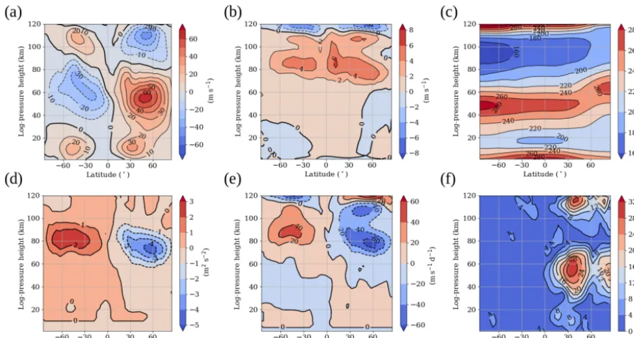
Figure 1.January zonal and monthly mean of the(a)zonal wind (m s−1),(b)meridional wind (m s−1),(c)temperature (K),(d)zonal GW fluxes (m2s−2),(e)zonal wind acceleration due to breaking GWs (m s−1d−1) and(f)SPW 1 amplitude (m s−1) extracted from the zonal wind of the reference simulation.
a geometrical height between 300 and 400 km. In the low-ermost 10 km, zonal mean temperatures are nudged to the 2000–2010 mean monthly mean ERA-Interim (Dee et al., 2011) zonal mean temperatures to correct the climatology of the troposphere, which is not included in the model in detail (Jacobi et al., 2015; Lilienthal et al., 2018). Furthermore, at 1000 hPa, which defines the lower boundary of the model, SPWs with wave numbers 1, 2 and 3 are forced, which are extracted from the 2000–2010 mean ERA-Interim monthly temperature and geopotential reanalysis data. The horizon-tal resolution of the model is 5◦ in latitude and 5.625◦ in longitude and the vertical resolution is 2.842 km. The model solves the primitive equations in flux form (e.g., Jakobs et al., 1986). MUAM includes parameterizations to simulate sub-grid processes such as GWs, absorption of solar radiation or infrared cooling. The absorption of radiation is realized ac-cording to Strobel (1986). This parameterization is focused on the absorption processes due to trace gases such as H2O (absorber in the troposphere) as well as CO2 and O3 (ab-sorbers in the stratosphere). Water vapor and ozone fields are prescribed. The heating rates are calculated by absorption bands representing the wavelength interval at which these trace gases absorb the atmospheric radiation. The infrared emission of CO2is parameterized following Fomichev et al. (1998), and ozone infrared cooling in the 9.6 µm band is cal-culated following Fomichev and Shved (1985).
GWs are parameterized after an updated linear scheme (Lindzen, 1981; Jakobs et al., 1986) with multiple break-ing levels (Fröhlich et al., 2003b; Jacobi et al., 2006). GW
amplitudes are included at an altitude of 10 km as a zonal mean with a global average of 1 cm s−1for the vertical ve-locity perturbation. This value is weighted by a prescribed zonal mean GW amplitude distribution based onEpot data obtained from GPS radio occultation measurements (Šácha et al., 2015; Lilienthal et al., 2017). Although theEpotdata still contain Kelvin waves and other possible wave struc-tures with short vertical wavelengths, which may introduce biases, the GW amplitude distribution is more realistic than the hyperbolic tangent function of the latitude, which was used in earlier experiments (Jacobi et al., 2006), and leads to an improvement of the zonal mean GW climatology. It shows maximum GW amplitudes (not shown here) at the Equator (convectively generated GWs) and at midlatitudes (orographically induced GWs). At each grid point 48 waves are induced that propagate in eight different directions with six different phase speeds ranging from 5 to 30 m s−1.
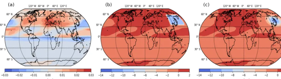
Figure 2. Zonal GW drag (m s−1d−1) at 26.9 km for the reference(a)and the H3 hotspot simulation as a box(b) and as a Gaussian distribution(c)for the last 30 d of analysis. Note the different scale for panel(a).
the spin-up period was modeled. Šácha et al. (2016) have al-ready analyzed the effect of the Asian hotspot with MUAM by performing a sensitivity study with regard to the strength of the GW forcing in the stratosphere. Their analysis time period was much shorter and the declination of the sun was different. They also nudged the model zonal mean tempera-ture up to 30 km. In this regard, our experimental setup might be considered superior to their simulations, especially as the nudging does not interfere with the GW forcing implemented in this new configuration. We refer to this reference simula-tion as “Ref”.
The state of the middle atmosphere in the Ref simula-tion can be seen in Fig. 1, which shows the January zonal mean zonal (Fig. 1a) and meridional wind (Fig. 1b), the temperature (Fig. 1c), zonal GW flux (Fig. 1d), the zonal wind acceleration due to breaking GWs (Fig. 1e), and the SPW 1 amplitude extracted from the zonal wind (Fig. 1f) as latitude–height plots. Each parameter is presented up to an altitude of 120 km for the winter and summer hemisphere. The zonal wind in Fig. 1a generally reproduces reference cli-matologies like CIRA-86 (Fleming et al., 1988) or URAP (Swinbank and Ortland, 2003), but the winter mesospheric jet is overestimated by about 10–20 m s−1. The meridional circulation (Fig. 1b) extending from the summer to the win-ter mesopause has a maximum of 6 m s−1 at about 80 km, which reproduces predictions by climatologies well (Port-nyagin et al., 2004; Jacobi et al., 2009). Temperature (Fig. 1c) generally reproduces climatology values. The GW fluxes (Fig. 1d) maximize at about 80 km, with a maximum of slightly above−4 m2s−2in the Northern Hemisphere (NH) and 2 m2s−2 in the Southern Hemisphere (SH). The cor-responding zonal GW drag maximizes at the same altitude with about −60 m s−1d−1 (40 m s−1d−1) in the NH (SH) and is directed westward (eastward). The SPW 1 amplitude (Fig. 1f) extracted from the zonal wind shows maximum val-ues at the border of the mesospheric jet maximum north of 30◦N between 50 and 60 km and in the polar region. This fits quite well with observations, but the amplitudes are slightly
underestimated due to the overestimated mesospheric jet, fil-tering some of the SPWs (Xiao et al., 2009).
2.2 Experiment description
Firstly, we reproduced the experiment of Šácha et al. (2016) to check if we still obtained similar results with the slightly modified setup. To represent the Asian GW breaking hotspot in the model, we enhanced the GW drag after model day 270, i.e., after the spin-up, and ran the model for 120 d as in the Ref simulation. Hence, the zonal (GWDu) and meridional
(GWDv) GW drag and the heating due to breaking GWs
(GWDT) were modified in the specific region of the observed
GW breaking hotspot. In principle, the response to the GW drag would in turn alter the GW propagation and breaking conditions and, thus, the GW drag and its distribution. To avoid those feedback mechanisms, the GW parameterization scheme is turned off during the experiments, and the model is fed with the GW drag field from the Ref simulation. How-ever, in the GW hotspot region, the GW drag is modified (as shown in Table 1). We intend to only analyze the steady-state impact of the local GW forcing that is not influenced by non-linear effects.
As in Šácha et al. (2016), we located the GW break-ing hotspot between 37.5 and 62.5◦N and between 118.1 and 174.3◦E in an altitude range between 18 and 30 km. Note that the geographic positions refer to the model grid points; thus, at a latitudinal 5◦ grid, the meridional size of the modeled hotspot is 30◦. To avoid a total breakdown of the polar vortex and a fundamental change in middle atmo-sphere dynamics, which was already forced in the study by Šácha et al. (2016), we chose the more moderate case of
−10 m s−1d−1 for GWDu, −0.1 m s−1d−1 for GWDv and
a warming of 0.05 K d−1 for GWDT. We refer to this
sim-ulation as the H3 simsim-ulation, as will be described later. The distribution of the GWDuof the Ref and the H3 simulations
not interested in short-term variabilities. The GWDu of the
Ref simulation varies between−0.025 and+0.02 m s−1d−1 in the GW hotspot region (27.5–87.5◦N, 118.1–174.3◦E, 18–30 km). Thus, the maximum value of the H3 simulation (GWDu= −10 m s−1d−1in the hotspot) is 500 times larger
than the maximum westward (negative) value of the Ref sim-ulation. The H3 mean value (mean GWDu:−10 m s−1d−1)
is roughly 3300 times larger than that of the Ref simula-tion (mean GWDu: 0.003 m s−1d−1) within the region of
the EA/NP hotspot. These maximum values of the GWDu
as well as those of the GWDv and the GWDT are
summa-rized in Table 1 for the Ref and the GW hotspot simula-tions. In spite of the huge difference compared with the Ref simulation, the zonal GW forcing is moderate in terms of what is estimated from observations (40 m s−1d−1and more) and from GW parameterizations in this region (Šácha et al., 2018). Concerning the meridional GW drag and the heating due to breaking GWs, the maximum (mean) value of the H3 simulation is only 5 (100) times larger than that of the Ref simulation (not shown here). To investigate possible effects with regard to the position of the GW hotspot, we performed a sensitivity study. For this, we kept the longitude (118.1– 174.3◦E) and altitude (18–30 km) range as well as the zonal extent of 25◦fixed, but varied the observed GW hotspot in 5◦steps from 27.5–52.5◦N (simulation H1) to 62.5–87.5◦N (simulation H8), while labeling the experiments in between as H2 through H7 (see Table 1).
To analyze the possible effects of the sharp transition zone between the unchanged and enhanced GW drag, additional simulations with a smoothed GW forcing were performed, using a 3-D Gaussian function with standard deviations of 10◦, 22.5◦ and 5.684 km in the zonal, meridional and ver-tical directions, respectively. To get the same integral forc-ing as in the H1–H8 simulations, the size or the intensity of the local GW forcing as a Gaussian distribution needed to be adjusted. For our experiments, we mainly increased the strength of the local GW forcing and only slightly increased the size. The maximum values for the GWDu, GWDv and
GWDT forcing as a 3-D Gaussian distribution were chosen
to be−13 m s−1d−1,−0.13 m s−1d−1and 0.065 K d−1(see Table 1), respectively. The 3-D Gaussian distribution for the H3 GW hotspot can be seen in Fig. 2c. In this paper we mainly concentrate on the 3-D GW hotspots shaped like a box when we analyze the effects on the middle atmosphere dynamics. For comparison, regarding the shape of the artifi-cial GW forcing, we just focus on the H3 GW hotspot with Gaussian smoothed boundaries when we discuss the SPW modulation in Sect. 3.2, which may be affected by the GW hotspots with sharp boundaries.
When comparing the size of the GW hotspots it is obvi-ous (can be seen in Fig. 5) that the area of the enhanced GW drag, which scales with the cosine of the latitude, decreases with increasing latitude. However, scaling the GW drag with latitude would lead to a much larger zonal mean GW drag at high latitudes and would result in changes in the
circula-tion. Furthermore, the horizontal winds, which are affected by resulting nonlinear interactions, are scaled in the model equations. In the current approach, we conserve the ratio of enhanced and unchanged GW drag values within the respec-tive latitudinal belt, which is more meaningful. Also, the hor-izontal wavelength of PWs becomes smaller with decreasing distance from the pole, meaning that the ratio of the width of the GW forcing and the horizontal wavelength of the PWs remains the same for the respective latitudinal belt. In the following, we will show that the spatial shape as well as the spatial size of the local GW forcing is not the most decisive factor when we compare the 3-D Gaussian distribution with the 3-D GW forcing shaped as a box. Thus, GW hotspots that are the same size may lead to comparable results.
3 Results
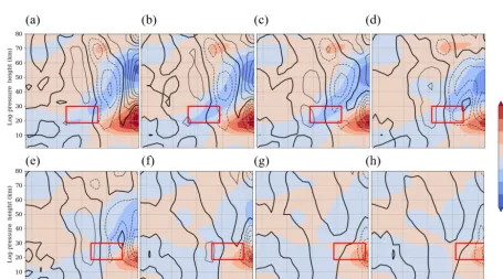
3.1 Hotspot effect on the background circulation Figure 3a–h show the zonal mean zonal wind difference be-tween each GW hotspot simulation H1–H8 and the Ref sim-ulation (in color) as well as the zonal mean zonal wind of the Ref simulation (as contour lines) in a latitude–height plot. The position of each GW hotspot is illustrated by a red box. All experiments (H1–H8) show negative zonal wind differences with a maximum wind decrease of more than
−10 m s−1 in the polar region. Positive differences can be observed equatorward from an imaginary line connecting the subtropical and polar-night jet centers, with a maximum dif-ference of 8 to 10 m s−1. These zonal wind anomalies are consistent with a polar vortex that is shifted towards lower latitudes, and the wind reversal in the mesosphere is shifted upwards at lower latitudes. The strongest decrease in the zonal mean zonal wind in the polar region can be observed in the H1 simulation (Fig. 3a) and the strongest increase in zonal mean zonal wind at lower latitudes can be observed in the H3 simulation (Fig. 3c), the latter corresponds to the observed Asian GW hotspot. For GW hotspots with a south-ern edge north of 50◦N, the polar vortex is only slightly displaced towards lower latitudes. Thus, the effect of GW hotspots at higher latitudes is not as strong.
Table 1.Overview of the mean and maximum values of the zonal and meridional GW drag and heating by GWs for the reference and hotspot simulations as a 3-D box (H1–H8) and as a Gaussian distribution (Gauss). The mean and maximum values refer to the region (118.1–174.3◦E, 18–30 km and the respective latitude range as listed below) of the hotspots.
Simulation Abbreviation Region Min/max GWDu Min/max GWDv Min/max GWDT
(m s−1d−1) (m s−1d−1) (K d−1)
Reference Ref -0.025/0.02 -0.025/0.01 -0.0006/0.01
Hotspots as 3-D box H1 27.5–52.5◦N −10 −0.1 0.05
H2 32.5–57.5◦N
H3 37.5–62.5◦N
H4 42.5–67.5◦N
H5 47.5–72.5◦N
H6 52.5–77.5◦N
H7 57.5–82.5◦N
H8 62.5–87.5◦N
118.1–174.3◦E 18–30 km
Hotspots as 3-D Gaussian distribution Gauss −13.1 −0.13 0.065
polar stratosphere. Above 35–40 km, we observe a positive vertical wind anomaly for the H1–H3 simulations, i.e., the downward movement is reduced and leads to an adiabatic cooling anomaly. For most of the simulations, the negative anomaly in the lower part of the stratosphere is stronger than the positive anomaly above 40 km, which fits with the distri-bution of the temperature anomalies. In case of the H4 and H5 simulations (Fig. 4d, e), the vertical wind anomalies do not fit with the temperature anomalies. We observe an in-creased downward movement in a region where the temper-ature weakly decreases.
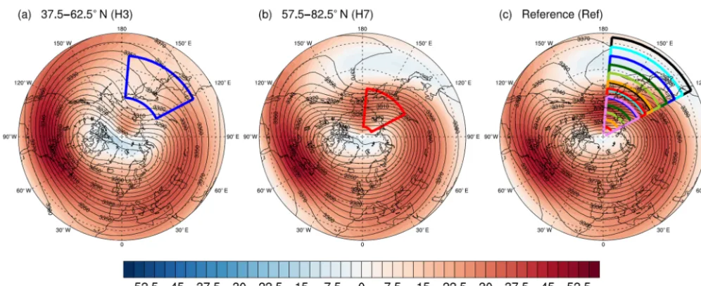
3.2 Influence on the polar vortex and anomalous SPWs From previous publications, it is already known that a warm-ing (coolwarm-ing) of the high-latitude stratosphere (mesosphere) and related changes in the dynamics are generally connected with PW activity. This leads us to the hypothesis that the main GWD enhancement effect is due to SPW modulation, and this will be investigated in this subsection. In Fig. 5, we show the geopotential height (as contour lines) and the zonal wind (using color coding) as a polar plot at 35 km, i.e., 5 km above the region of GW forcing, for the H3 (Fig. 5a), H7 (Fig. 5b) and Ref simulations (Fig. 5c). The panels rep-resent the last 30 d of analysis. The position of each GW hotspot is illustrated by the boxes, H1 (black) to H8 (vio-let), in Fig. 5c. The polar vortex of the Ref simulation is sta-ble (not displaced or split) and located near the North Pole (Fig. 5c). Between 30 and 55◦N, the zonal wind of the Ref simulation is easterly in one part of the EA/NP region due to the Aleutian High (AH). This means that the GW forc-ing, which normally acts against the westerly zonal mean zonal wind, locally strengthens the zonal wind. Between 55 and 90◦N there is a strong westerly wind between East Asia and Alaska; thus, the GW forcing there acts locally against
Figure 3.Zonal mean zonal wind difference between the H1–H8 simulations(a–h)and the reference simulation (H1–H8−Ref). The colors indicate the difference between the simulations, and the contour lines show the zonal mean zonal wind of the reference simulation. Figures represent the last 30 d of the simulations. The position of each GW hotspot is represented by a red box.
[image:7.612.66.522.403.656.2]Figure 5.Zonal wind (m s−1) in color and geopotential height (gpdam) as contour lines north of 25◦N at 35 km for the H3(a), H7(b)and the Ref(c)simulations, representing the last 30 d of analysis. The boxes illustrate the position of each GW hotspot: H1 (in black) to H8 (in violet). The blue(a, c)(red,b, c) box refers to the H3 (H7) simulation.
in the polar stratosphere of about 20 m s−1.With respect to the H1–H4 simulations, in Fig. 6a–d the zonal wind SPW 1 amplitude differences are positive (negative) on the north-ern (southnorth-ern) flank of the respective GW hotspot up to an altitude of about 60 km. The negative (positive) SPW 1 am-plitude anomaly increases (decreases) for more GW hotspots located further north. The strongest increase (decrease) in the SPW 1 amplitude can be observed in the H1 (H4) simulation, with more than 8 m s−1(−8 m s−1). By comparing the posi-tive and negaposi-tive SPW 1 amplitude anomalies of the H1–H4 simulations it can be seen that the positive anomaly is less pronounced, whereas the negative anomaly is more prevalent throughout the NH, particularly around the stratopause. The decreasing SPW 1 amplitude indicates that fewer SPWs 1 are propagating into the middle atmosphere. Due to the de-creasing SPW 1 activity at lower latitudes, fewer SPWs 1 are breaking in this region, i.e., the zonal mean zonal wind is less decelerated (as is shown in Fig. 3). Nonlocally, how-ever, a localized destructive (constructive) superposition of the original SPWs 1 within the model and that of the GW forcing may decrease (increase) the SPW 1 amplitude at other heights/latitudes due to changes in PW propagation. This effect can be seen around 55◦N, where we observe an enhanced SPW 1 amplitude. It is strongest for the H1 GW hotspot and decreases for GW hotspots located further north. The suppressed upward propagation of SPWs 1 leads to an increase in the SPW 1 amplitude in this area. This positive SPW 1 amplitude anomaly corresponds to the decelerated zonal mean zonal wind in Fig. 3. This leads to the assump-tion that the GW forcing may locally increase or decrease the SPW 1 amplitude, but prevents the SPWs from propagating upwards into higher altitudes; hence, the SPW 1 amplitude mainly decreases in the stratosphere/mesosphere. Thus, the
local GW forcing has a destructive effect on the circulation in the middle atmosphere.
We will verify this in Sect. 3.3 by analyzing the Eliassen– Palm flux. Owing to the suppression of SPW 1 propagation at midlatitudes, the SPWs may increasingly propagate via the polar region, which may explain the increased SPW 1 ampli-tude in the polar stratosphere north of 75◦N. Another posi-tive SPW 1 amplitude anomaly can be observed in the mid-latitudinal mesosphere above 60 km, which may be induced by local instabilities generating new SPWs 1. Both of these positive SPW 1 amplitude anomalies are strongest for the H1 simulation and once again decrease for northward-shifted GW hotspots. The SPW 1 amplitude anomalies for the four northernmost GW hotspots, H5–H8 in Fig. 6e–h, are small in comparison with the four southernmost GW hotspot sim-ulations, which correspond to the observations in Sect. 3.1. Only for the H5 simulation (Fig. 6e) is the SPW 1 activity also strongly reduced at lower latitudes above 30 km, as in the H1–H4 simulations.
Figure 6.Zonal mean SPW 1 amplitude extracted from the zonal wind as the difference between the H1–H8 simulations(a–h)and the reference simulation. The colors indicate the difference between the simulations, and the contour lines show the zonal mean SPW 1 amplitude of the reference simulation. Figures represent the last 30 d of the simulations. The position of each GW hotspot is represented by a red box.
largest decrease can be observed for the southernmost GW hotspot, and the decrease becomes smaller for northward-displaced GW hotspots. Only at lower latitudes is the SPW 2 amplitude slightly increasing for those simulations. This is the case for the H2, H3, H4 and H5 simulation. The SPW 2 anomaly is negative (positive) in the regions where the SPW 1 anomaly is positive (negative). This leads to the assumption that just one of both SPWs (SPW 1 and SPW 2) can be dom-inant. By comparing the latitudinal distribution of the SPW 1 and 2 amplitude anomalies northward of 30◦N, it can be seen that they are similar when we neglect the scales. Both show a decrease in amplitude around 40 and 70◦N and an increase in the midlatitudes and in the polar region. In comparison, the SPW 3 amplitude anomaly distribution (Fig. 7c) is slightly different, as the SPW 3 amplitude decreases at 20◦N (not at 40◦N, as seen for the SPW 1 and 2 anomalies). However, as for the SPW 1 and 2 anomalies, an increase in the SPW 3 amplitude induced by the local GW hotspots can be ob-served in the midlatitudes with a maximum of about 2 m s−1. The largest increase in SPW 3 amplitude can be seen in the H1 simulation (southernmost GW hotspot), and the largest decrease is observed in the H3 simulation (observed Asian GW hotspot).
The suppression of SPWs, which is induced by the local GW forcing, might also be an effect partly induced by the shape of the GW hotspot, leading to a sharp transition zone between the unchanged and enhanced GW drag values. To prove that the shape of the GW hotspot partly leads to a
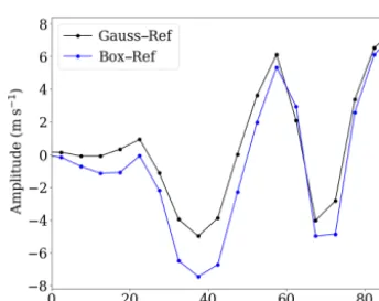
sup-pression of SPWs, Fig. 8 shows the H3 amplitude anomaly from Fig. 7a and the corresponding Gauss simulation de-scribed in Sect. 2. The latitudinal distribution of the SPW 1 amplitude difference is still the same, showing the two lo-cal maxima at the midlatitudes and in the polar region and the two minima at 40 and 70◦N, although these two minima decreased from −8 m s−1 for the 3-D box to−4 m s−1 for the Gaussian distribution. Moreover, the maxima increased from about 4 m s−1to more than 5 m s−1. Due to the stronger maximum GW drag in the Gaussian distribution the SPW 1 excitation is strengthened, which leads to the larger SPW 1 amplitudes at midlatitudes. The smoothly decreasing GW drag forcing towards lower and higher latitudes only slightly reduces the suppression of SPW 1 around 40 and 70◦N. The mean wind and temperatures are also only weakly affected if we replace the box-like forcing with one with a Gaussian shape (not shown here). Thus, the GW hotspot itself leads to essential changes in the dynamics, suppressing the SPW propagation and decreasing the SPW 1 activity in the middle atmosphere.
Figure 7.Zonal mean SPW 1(a), SPW 2(b)and SPW 3(c)amplitudes as the difference between the H1–H8 simulations and the Ref simulation at 35 km for the last 30 d of the simulations extracted from the zonal wind.
Figure 8.SPW 1 amplitude as the difference between the H3 sim-ulation and the reference simsim-ulation (blue line) and the Gauss dis-tribution and the reference simulation (black line) at 35 km for the last 30 d extracted from the zonal wind.
propagation show that the GW drag can play an important role in preconditioning the polar vortex (see next section).
3.3 Propagation conditions for SPWs
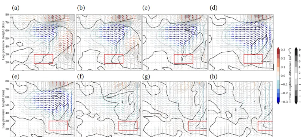
To establish the extent to which the SPW propagation is af-fected by the local GW forcing, the EP fluxes and their di-vergence for SPW 1 were calculated. The results of the Ref simulation are presented in Fig. 9a. The arrows show the di-rection of propagation, the color of the arrows represents the strength of the EP flux not normalized by the density, and the grey areas and the grey contour lines represent the EP diver-gence, showing the direction in which the zonal mean flow is accelerated. A negative (positive) EP divergence is illus-trated by the dashed (solid) lines. The arrows were replaced by dots when the amplitude difference was smaller than 1 % of the maximum EP flux amplitude difference. The waves mainly develop in the middle and higher latitudes, and from there they mainly propagate towards the equatorial strato-sphere/stratopause and, to a much lesser degree, to the polar stratosphere. That the waves are really propagating upwards can be seen by means of the increasing amplitudes of the
EP fluxes. The maximum EP flux amplitudes of more than 1.4 m2s−2are reached between 50 and 60◦N at an altitude of about 60 km, which corresponds to the height of the SPW 1 amplitude maximum in Fig. 1f of the Ref simulation.
[image:10.612.81.253.244.380.2]Figure 9. Zonal mean EP flux of SPW 1 of the Ref simulation(a). Contour lines show the EP flux divergence, and dashed lines denote negative EP flux divergence. The refractive index for SPW 1 for the Ref simulation(b)with a thicker zero line. The position of the H3 (H7) GW hotspot and the respective zero line is represented by the dashed (dotted) violet line. Both panels represent the last 30 d of the simulation.
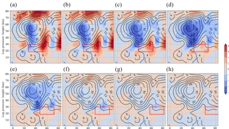
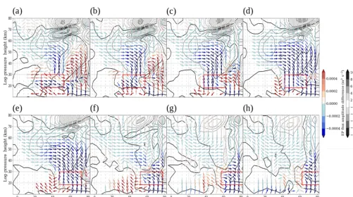
Figure 10.Zonal mean EP flux (arrows) and divergence (isolines and shaded areas; dashed lines show negative values) of SPW 1. Shown is the difference between all H1–H8 simulations(a–h)and the reference simulation (H1–H8−Ref) representing the last 30 d of the simulations.
the positive EP divergence) due to the reversed wind con-ditions. The mesospheric EP flux in the H1–H5 simulations corresponds to the observed enhanced SPW 1 amplitude in the mesosphere in Fig. 7. Referring to the enhanced SPW 1 around 55◦N of the GW hotspots, no enhanced EP flux can be observed in the respective region. However, the ar-rows of the EP flux anomalies are pointing towards this area of enhanced SPW 1 amplitude. In the H6–H8 GW hotspot simulations (Fig. 10f–h) no large differences in EP flux and divergence occur, which correspond to the small SPW 1 am-plitude and the zonal mean zonal wind differences in Figs. 7 and 3.
To explain why SPWs 1 do not propagate at higher lati-tudes, the refractive index (Matsuno, 1971; Andrews et al., 1987), multiplied by the square of the Earth’s radius a2, is
also shown in Fig. 9b. The refractive index is highly depen-dent on the meridional potential vorticity gradient (qy) and
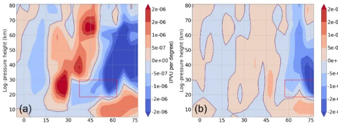
[image:11.612.48.548.250.478.2]Figure 11.Meridional potential vorticity gradient difference between the respective H3(a)and H7(b)simulations and the reference simula-tion, representing the last 30 d of the simulations. The positions of the H3 and H7 GW hotspots are represented by red boxes.
index changes after the implementation of the GW forcing, the position of the H3 (dashed violet line) and the H7 (dotted violet line) GW hotspot and the respective zero line of the refractive index were added to Fig. 9b. In the H3 simulation, the zero line is higher in the polar region than in the Ref sim-ulation. Thus, the refractive index increases (becomes more positive) in the polar region below 30 km, which corresponds to the enhanced SPW 1 propagation and SPW 1 amplitude in the same region. The zero line of the H7 simulation is almost at the same height as that of the Ref simulation; thus, we do not observe huge changes in the Arctic. While the zero line of the Ref simulation is limited to the regions north of 60◦N, the zero line of the H3 (H7) simulation is located around 50◦N (57◦N). Based on the EP flux distribution of the Ref simu-lation in Fig. 9a, we already know that the SPWs 1 mainly propagate from the midlatitudes (between 50 and 60◦N) into the middle atmosphere. Due to the negative refractive index in this region, the SPWs 1 in the H3 and H7 simulations are no longer able to propagate upwards, meaning that the SPW 1 EP flux and amplitude decrease. Thus, the major branch of SPW 1 propagation is interrupted by the local GW forc-ing. To check if there are local instabilities leading to the SPW 1 sources in the polar region and in the lower meso-sphere, theqydifferences between the H3 (H7) and the Ref
simulation are shown in Fig. 11. The qy is given in
poten-tial vorticity units (PVU) per degree. The positions of the H3 and H7 GW hotspot are illustrated using red boxes. Due to the increasing (decreasing) zonal mean zonal wind at lower (higher) latitudes, theqy, which normally increases towards
higher latitudes, is reversed northward of 30◦N. We observe a negativeqyanomaly, which is tilted towards the north with
increasing height. Northward of 45◦N up to 20 km theqy
anomaly reverses again and becomes positive. These local reversals of theqy, which are a necessary condition for
baro-clinic instability (Charney and Stern, 1962), can lead to the SPW 1 sources and positive EP divergences in the respective regions.
4 Conclusions
The sensitivity study regarding the effect of local GW hotspots in the stratosphere from lower to higher latitudes in a specific longitude range (between 120 and 170◦E) shows that GW hotspots south of 50◦N lead to a negative refrac-tive index at midlatitudes, which prevents the SPWs from propagating upwards. Thus, fewer SPWs 1 are breaking in the middle atmosphere corresponding to the decreasing SPW 1 amplitude at lower latitudes connected with an increasing zonal mean zonal wind. Thus, the polar vortex is shifted to-wards lower latitudes but remains very strong (Baldwin and Holton, 1988), which additionally leads to a suppression of SPWs according to the Charney–Drazin criterion (Charney and Drazin, 1961). The displacement of the polar vortex in-duced by breaking SPWs 1 causes an increase in the refrac-tive index in the polar stratosphere (Karami et al., 2016); thus, the SPWs 1 originating at midlatitudes partly propagate via the polar region into the middle atmosphere. Apart from these SPWs 1, additional SPWs 1 propagating upwards are directly generated in the Arctic owing to local baroclinic in-stability; one indication of this is the reversal of theqy
(Char-ney and Stern, 1962; Garcia, 1991). For this reason we ob-serve an enhanced EP flux and, thus, an enhanced SPW 1 amplitude in the polar region. These SPWs 1 break around 50 km between 50 and 80◦N and lead to an enhanced nega-tive EP divergence connected with a decrease in zonal mean zonal wind at higher latitudes. In the lower mesosphere be-tween 40 and 70◦N there is a second source of SPWs 1 (pos-itive EP divergence) in addition to local baroclinic instabili-ties (reversal of theqy) (Smith, 2003; Lieberman et al., 2013;
wind conditions, shows negative values in the polar region for the Ref simulation. Thus, if we implement a GW forcing directly in this region it has no impact on the middle atmo-sphere as SPWs cannot propagate. If we provoke precondi-tioning of the polar vortex by first implementing, for exam-ple, the H1 GW hotspot and then adding one of the H6–H8 GW hotspots, the GW hotspots near the polar region would have a larger impact on the dynamics of the middle atmo-sphere.
Based on the results of the sensitivity study, we see that a local GW forcing can lead to a weakening (warming of the lower stratosphere) and slight displacement of the polar vortex at high latitudes, which is highly dependent on the strength (Šácha et al., 2016) and the zonal distribution of the forcing (this study). Usually, it is assumed that precon-ditioning of the polar vortex is mainly driven by enhanced PW activity (Labitzke, 1981). However, there are also sev-eral indications based on satellite observations (Ern et al., 2016) and reanalysis data (Albers and Birner, 2014) which show that the GW drag and the absolute GW momentum flux is enhanced (reduced) in the stratosphere right before (after) SSWs. Albers and Birner (2014) analyzed the total wave forcing from the Japanese Meteorological Agency and Central Research Institute of Electrical Power Industry 25-year Reanalysis (JRA-25) data before SSW events and found that up to 70 % of the total drag is induced by orographic GWs. Ern et al. (2016) directly derived the GW drag and ab-solute momentum fluxes from HIRDLS and SABER temper-atures and found that both parameters are enhanced before and around the central day of a SSW (strong polar jet), and they are reduced when the zonal wind is weak (after SSW). Because we kept the GW drag forcing constant throughout the experiment we cannot evaluate nonlinear effects, which would possibly reduce the GW drag connected with the dis-placement of the polar vortex. Furthermore, we have a fixed GW source distribution, meaning that no additional GWs are generated owing to changes in the tropospheric circulation. Nevertheless, on the basis of the zonal and meridional GW flux, which changes according to the propagation conditions, we analyzed the absolute horizontal GW momentum flux (not shown here). In this case, we also observe a reduction in the GW flux when the zonal mean zonal wind decreases at high latitudes. However, this effect is not very pronounced in our experiments, as the zonal mean zonal wind differences are much smaller than during a real SSW event. We only ob-serve zonal mean zonal wind differences of about−10 m s−1, which do not lead to a reversal of the zonal mean zonal wind or to subsequent significant background changes that may strongly influence the GW propagation.
Another interesting aspect is that different local GW forc-ing shapes do not have strong effects on the circulation. In spite of the Gaussian-smoothed boundaries, only negligible changes can be observed in the dynamics and SPW develop-ment, which are mainly due to the varying GW drag in the 3-D Gaussian distribution, leading to larger (smaller) effects when the Gaussian distribution reaches a maximum (mini-mum).
Comparing the positions of these simulated GW hotspots with measurements (e.g., Hoffmann et al., 2013), it is clear that at least some of the latitudinally shifted GW hotspots are not very realistic; therefore, our experiments should only be considered as a qualitative sensitivity study. Regarding orog-raphy, there are no obvious sources of orography when we displace the GW hotspot latitudinally. However, some of the GW hotspots can connect to jet exit regions on a purely hy-pothetical basis. To make the study more realistic, the next step would be to analyze the effect of a longitudinally shifted hotspot (fixed latitude range between 30 and 60◦N), as ob-servations and GCM experiments have shown their existence (listed in the introduction). In this latitude range GW hotspots like the Himalayan region, the Alps or the Rocky mountains are included in the experiments. Also, the interaction of two or more GW hotspots is one of our focuses and will provide more insight into the effect of a localized GW forcing, which may be also important for the development of new GW pa-rameterizations.
Appendix A
Author contributions. NS performed the MUAM model simula-tions and drafted the first version of the paper. PŠ provided the GW potential energy distributions. PŠ, PP, AK and CJ actively con-tributed to the discussions and to writing the paper.
Competing interests. Christoph Jacobi is one of the editors in chief ofAnnales Geophysicae. The authors declare that there are no con-flicts of interest.
Special issue statement. This article is part of the special issue “Vertical coupling in the atmosphere–ionosphere system”. It is a result of the 7th Vertical coupling workshop, Potsdam, Germany, 2–6 July 2018.
Acknowledgements. ERA-Interim reanalysis data were provided by ECMWF via the following website: https://www.ecmwf. int/en/forecasts/datasets/browse-reanalysis-datasets (last access: 27 June 2019).
Financial support. This research has been supported by the
Deutsche Forschungsgemeinschaft (DFG; grant no. JA836/32-1) and by GA CR (grant no. 16-01562J). Petr Pišoft and Aleš Kuchaˇr were supported by GA CR (grant nos. 16-01562J and 18-01625S). Petr Šácha was supported by GA CR (grant nos. 16-01562J and 18-01625S) and by the Government of Spain (grant no. CGL2015-71575-P) as well as via a postdoctoral grant from the Xunta de Gali-cia (grant no. ED481B 2018/103) in the later stages of the paper preparation. The EPhysLab is supported through the European Re-gional Development Fund (ERDF).
Review statement. This paper was edited by Kathrin Baumgarten and reviewed by two anonymous referees.
References
Albers, J. R. and Birner, T.: Vortex Preconditioning due to Planetary and Gravity Waves prior to Sudden Stratospheric Warmings, J. Atmos. Sci., 71, 4028–4054, https://doi.org/10.1175/JAS-D-14-0026.1, 2014.
Alexander, P., Luna, D., Llamedo, P., and de la Torre, A.: A grav-ity waves study close to the Andes mountains in Patagonia and Antarctica with GPS radio occultation observations, Ann. Geo-phys., 28, 587–595, https://doi.org/10.5194/angeo-28-587-2010, 2010.
Andrews, D. G., Holton, J. R., and Leovy, C. B.: Middle Atmo-sphere Dynamics, ISBN 0-12-058576-6, Academic Press, San Diego, 1987.
Baldwin, M. P. and Holton, J. R.: Climatology of the stratospheric polar vortex and planetary wave breaking, J. Atmos. Sci., 45, 1123–1142, https://doi.org/10.1175/1520-0469(1988)045<1123:COTSPV>2.0.CO;2, 1988.
Charney, J. G. and Drazin, P. G.: Propagation of planetary-scale dis-turbances from the lower into the upper atmosphere, J. Geophys. Res., 66, 83–109, https://doi.org/10.1029/JZ066i001p00083, 1961.
Charney, J. G. and Stern, M. E.: On the Stability of In-ternal Baroclinic Jets in a Rotating Atmosphere, J. At-mos. Sci., 19, 159–172, https://doi.org/10.1175/1520-0469(1962)019<0159:OTSOIB>2.0.CO;2, 1962.
Costantino, L., Heinrich, P., Mzé, N., and Hauchecorne, A.: Convective gravity wave propagation and breaking in the stratosphere: comparison between WRF model simu-lations and lidar data, Ann. Geophys., 33, 1155–1171, https://doi.org/10.5194/angeo-33-1155-2015, 2015.
Dee, D. P., Uppala, S. M., Simmons, A. J., Berrisford, P., Poli, P., Kobayashi, S., Andrae, U., Balmaseda, M. A., Balsamo, G., Bauer, P., Bechtold, P., Beljaars, A. C. M., van de Berg, L., Bid-lot, J., Bormann, N., Delsol, C., Dragani, R., Fuentes, M., Geer, A. J., Haimberger, L., Healy, S. B., Hersbach, H., Hólm, E. V., Isaksen, L., Kallberg, P., Köhler, M., Matricardi, M., McNally, A. P., Monge-Sanz, B. M., Morcrette, J.-J., Park, B.-K., Peubey, C., de Rosnay, P., Tavolato, C., Thépaut, J.-N., and Vitart, F.: The ERA-Interim reanalysis: configuration and performance of the data assimilation system, Q. J. Roy. Meteor. Soc., 137, 553–597, https://doi.org/10.1002/qj.828, 2011.
Douville, H.: Stratospheric polar vortex influence on Northern Hemisphere winter climate variability, Geophys. Res. Lett., 36, L18703, https://doi.org/10.1029/2009GL039334, 2009. Ern, M. and Preusse, P.: Gravity wave momentum flux spectra
observed from satellite in the summertime subtropics: Impli-cations for global modeling, Geophys. Res. Lett., 39, L15810, https://doi.org/10.1029/2012GL052659, 2012.
Ern, M., Preusse, P., Alexander, M. J., and Warner, C. D.: Absolute values of gravity wave momentum flux de-rived from satellite data, J. Geophys. Res., 109, D20103, https://doi.org/10.1029/2004JD004752, 2004.
Ern, M., Ploeger, F., Preusse, P., Gille, J. C., Gray, L. J., Kalisch, S., Mlynczak, M. G., Russell III, J. M. R., and Riese, M.: Interaction of gravity waves with the QBO: A satel-lite perspective, J. Geophys. Res.-Atmos., 119, 2329–2355, https://doi.org/10.1002/2013JD020731, 2014.
Ern, M., Trinh, Q. T., Kaufmann, M., Krisch, I., Preusse, P., Unger-mann, J., Zhu, Y., Gille, J. C., Mlynczak, M. G., Russell III, J. M., Schwartz, M. J., and Riese, M.: Satellite observations of middle atmosphere gravity wave absolute momentum flux and of its vertical gradient during recent stratospheric warmings, At-mos. Chem. Phys., 16, 9983–10019, https://doi.org/10.5194/acp-16-9983-2016, 2016.
Fleming, E. L., Chandra, S., Barnett, J. J., and Corney, M.: Zonal mean temperature, pressure, zonal wind and geopoten-tial height as functions of latitude, Adv. Space Res., 10, 11–59, https://doi.org/10.1016/0273-1177(90)90386-E, 1988.
Fomichev, V. I. and Shved, G. M.: Parameterization of the radiative flux divergence in the 9.6 µm O3 band, J. Atmos. Terr. Phys., 47, 1037–1049, https://doi.org/10.1016/0021-9169(85)90021-2, 1985.
Fritts, D. C. and Alexander, M. J.: Gravity wave dynamics and effects in the middle atmosphere, Rev. Geophys., 41, 1003, https://doi.org/10.1029/2001RG000106, 2003.
Fröhlich, K., Pogoreltsev, A., and Jacobi, C.: Numerical simulation of tides, Rossby and Kelvin waves with the COMMA-LIM model, Adv. Space Res., 32, 863–868, https://doi.org/10.1016/S0273-1177(03)00416-2, 2003a. Fröhlich, K., Pogoreltsev, A., and Jacobi, C.: The 48-layer
COMMA-LIM model, Rep. Inst. Meteorol. Univ. Leipzig, 30, 157–185, available at: http://nbn-resolving.de/urn:nbn:de:bsz: 15-qucosa-217766 (last access: 27 June 2019), 2003b.
Fröhlich, K., Schmidt, T., Ern, M., Preusse, P., de la Torre, A., Wickert, J., and Jacobi, C.: The global distribution of gravity wave energy in the lower stratosphere de-rived from GPS data and gravity wave modelling: attempt and challenges, J. Atmos. Sol.-Terr. Phy., 69, 2238–2248, https://doi.org/10.1016/j.jastp.2007.07.005, 2007.
Garcia, R. R.: Parameterization of planetary wave breaking in the middle atmosphere, J. Atmos. Sci., 48, 1405–1419, https://doi.org/10.1175/1520-0469(1991)048<1405:POPWBI>2.0.CO;2, 1991.
Hierro, R., Steiner, A. K., de la Torre, A., Alexander, P., Llamedo, P., and Cremades, P.: Orographic and convective gravity waves above the Alps and Andes Mountains during GPS radio occulta-tion events – a case study, Atmos. Meas. Tech., 11, 3523–3539, https://doi.org/10.5194/amt-11-3523-2018, 2018.
Hoffmann, L., Xue, X., and Alexander, M. J.: A global view of stratospheric gravity wave hotspots located with Atmospheric Infrared Sounder observations, J. Geophys. Res., 118, 416–434, https://doi.org/10.1029/2012JD018658, 2013.
Holton, J. R.: The role of gravity wave induced drag and diffusion in the momentum budget of the mesosphere, J. Atmos. Sci., 39, 791–799, https://doi.org/10.1175/1520-0469(1982)039<0791:TROGWI>2.0.CO;2, 1982.
Jacobi, C., Fröhlich, K., and Pogoreltsev, A.: Quasi two-day-wave modulation of gravity wave flux and conse-quences for the planetary wave propagation in a simple circulation model, J. Atmos. Sol.-Terr. Phy., 68, 283–292, https://doi.org/10.1016/j.jastp.2005.01.017, 2006.
Jacobi, C., Fröhlich, K., Portnyagin, Y., Merzlyakov, E., Solovjova, T., Makarov, N., Rees, D., Fahrutdinova, A., Guryanov, V., Fe-dorov, D., Korotyshkin, D., Forbes, J., Pogoreltsev, A., and Kürschner, D.: Semi-empirical model of middle atmosphere wind from the ground to the lower thermosphere, Adv. Space Res., 43, 239–246, https://doi.org/10.1016/j.asr.2008.05.011, 2009.
Jacobi, C., Lilienthal, F., Geißler, C., and Krug, A.: Long-term vari-ability of mid-latitude mesosphere-lower thermosphere winds over Collm (51◦N, 13◦E), J. Atmos. Sol.-Terr. Phy., 136, 174– 186, https://doi.org/10.1016/j.jastp.2015.05.006, 2015.
Jakobs, H. J., Bischof, M., Ebel, A., and Speth, P.: Simulation of gravity wave effects under solstice conditions using a 3-D cir-culation model of the middle atmosphere, J. Atmos. Terr. Phys., 48, 1203–1223, https://doi.org/10.1016/0021-9169(86)90040-1, 1986.
Jiang, J. H., Wang, B., Goya, K., Hocke, K., Eckermann, S. D., Ma, J., Wu, D. L., and Read, W. J.: Geographical distribution and interseasonal variability of tropical deep convection: UARS
MLS observations and analyses, J. Geophys. Res., 109, D03111, https://doi.org/10.1029/2003JD003756, 2004.
Karami, K., Braesicke, P., Sinnhuber, M., and Versick, S.: On the climatological probability of the vertical propagation of sta-tionary planetary waves, Atmos. Chem. Phys., 16, 8447–8460, https://doi.org/10.5194/acp-16-8447-2016, 2016.
Kirkwood, S., Mihalikova, M., Rao, T. N., and Satheesan, K.: Tur-bulence associated with mountain waves over Northern Scan-dinavia – a case study using the ESRAD VHF radar and the WRF mesoscale model, Atmos. Chem. Phys., 10, 3583–3599, https://doi.org/10.5194/acp-10-3583-2010, 2010.
Kumar, K., Ramkumar, T. K., and Krishnaiah, M.: Analy-sis of large-amplitude stratospheric mountain wave event ob-served from the AIRS and MLS sounders over the west-ern Himalayan region, J. Geophys. Res., 117, D22102, https://doi.org/10.1029/2011JD017410, 2012.
Labitzke, K.: The Amplification of Height Wave 1 in January 1979: A Characteristic Precondition for the Major Warming in February, Mon. Weather Rev., 109, 983–989, https://doi.org/10.1175/1520-0493(1981)109<0983:TAOHWI>2.0.CO;2, 1981.
Li, Q., Graf, H.-F., and Giorgetta, M. A.: Stationary planetary wave propagation in Northern Hemisphere winter – climatological analysis of the refractive index, Atmos. Chem. Phys., 7, 183– 200, https://doi.org/10.5194/acp-7-183-2007, 2007.
Lieberman, R. S., Riggin, D. M., and Siskind, D. E.: Stationary waves in the wintertime mesosphere: Evidence for gravity wave filtering by stratospheric planetary waves, J. Geophys. Res., 118, 3139–3149, https://doi.org/10.1002/jgrd.50319, 2013.
Lilienthal, F., Jacobi, C., Schmidt, T., de la Torre, A., and Alexan-der, P.: On the influence of zonal gravity wave distributions on the Southern Hemisphere winter circulation, Ann. Geophys., 35, 785–798, https://doi.org/10.5194/angeo-35-785-2017, 2017. Lilienthal, F., Jacobi, C., and Geißler, C.: Forcing mechanisms
of the terdiurnal tide, Atmos. Chem. Phys., 18, 15725–15742, https://doi.org/10.5194/acp-18-15725-2018, 2018.
Lilly, D. K., Nicholls, J. M., Kennedy, P. J., Klemp, J. B., and Chervin, R. M.: Aircraft measurements of wave momentum flux over the Colorado Rocky mountains, Q. J. Roy. Meteor. Soc., 108, 625–641, https://doi.org/10.1002/qj.49710845709, 1982. Lindzen, R. S.: Turbulence and stress owing to gravity wave
and tidal breakdown, J. Geophys. Res., 86, 9707–9714, https://doi.org/10.1029/JC086iC10p09707, 1981.
Llamedo, P., de la Torre, A., Luna, P. A. D., Schmidt, T., and Wickert, J.: A gravity wave analysis near the Andes range from GPS radio occultation data and mesoscale numerical sim-ulations: Two case studies, Adv. Space Res., 44, 494–500, https://doi.org/10.1016/j.asr.2009.04.023, 2009.
Matsuno, T.: A dynamical model of the strato-spheric sudden warming, J. Atmos. Sci., 28, 1479–1494, https://doi.org/10.1175/1520-0469(1971)028<1479:ADMOTS>2.0.CO;2, 1971.
Matthias, V. and Ern, M.: On the origin of the meso-spheric quasi-stationary planetary waves in the unusual Arc-tic winter 2015/2016, Atmos. Chem. Phys., 18, 4803–4815, https://doi.org/10.5194/acp-18-4803-2018, 2018.
strato-sphere over an Antarctic Peninsula station, J. Geophys. Res., 116, D14111, https://doi.org/10.1029/2010JD015349, 2010. Nastrom, G. D. and Fritts, D. C.: Sources of Mesoscale
Vari-ability of Gravity Waves. Part I: Topographic Excitation, J. Atmos. Sci., 49, 101–110, https://doi.org/10.1175/1520-0469(1992)049<0101:SOMVOG>2.0.CO;2, 1992.
Pišoft, P., Šácha, P., Miksovsky, J., Huszar, P., Scherllin-Pirscher, B., and Foelsche, U.: Revisiting internal gravity waves analy-sis using GPS RO density profiles: comparison with temperature profiles and application for wave field stability study, Atmos. Meas. Tech., 11, 515–527, https://doi.org/10.5194/amt-11-515-2018, 2018.
Plougonven, R. and Zhang, F.: Internal gravity waves from atmospheric jets and fronts, Rev. Geophys., 52, 33–76, https://doi.org/10.1002/2012RG000419, 2014.
Plougonven, R., Hertzog, A., and Teitelbaum, H.: Observations and simulations of a large-amplitude mountain wave breaking over the Antarctic Peninsula, J. Geophys. Res., 113, D16113, https://doi.org/10.1029/2007JD009739, 2008.
Pogoreltsev, A. I., Vlasov, A. A., Fröhlich, K., and Ja-cobi, C.: Planetary waves in coupling the lower and up-per atmosphere, J. Atmos. Solar-Terr. Phys., 69, 2083–2101, https://doi.org/10.1016/j.jastp.2007.05.014, 2007.
Portnyagin, Y., Solovjova, T., Merzlyakov, E., Forbes, J., Palo, S., Ortland, D., Hocking, W., MacDougall, J., Thayaparan, T., Manson, A., Meek, C., Hoffmann, P., Singer, W., Mitchell, N., Pancheva, D., Igarashi, K., Murayama, Y., Jacobi, C., Kürschner, D., Fahrutdinova, A., Korotyshkin, D., Clark, R., Tai-lor, M., Franke, S., Fritts, D., Tsuda, T., Nakamura, T., Gu-rubaran, S., Rajaram, R., Vincent, R., Kovalam, S., Batista, P., Poole, G., Malinga, S., Fraser, G., Murphy, D., Riggin, D., Aso, T., and Tsutsumi, M.: Mesosphere/lower thermo-sphere prevailing wind model, Adv. Space Res., 34, 1755–1762, https://doi.org/10.1016/j.asr.2003.04.058, 2004.
Reid, I. M. and Vincent, R. A.: Measurements of mesospheric gravity wave momentum fluxes and mean flow accelerations at Adelaide, Australia, J. Atmos. Terr. Phys., 49, 443–460, https://doi.org/10.1016/0021-9169(87)90039-0, 1987.
Šácha, P., Kuchaˇr, A., Jacobi, C., and Pišoft, P.: Enhanced internal gravity wave activity and breaking over the northeastern Pacific– eastern Asian region, Atmos. Chem. Phys., 15, 13097–13112, https://doi.org/10.5194/acp-15-13097-2015, 2015.
Šácha, P., Lilienthal, F., Jacobi, C., and Pišoft, P.: Influence of the spatial distribution of gravity wave activity on the middle at-mospheric dynamics, Atmos. Chem. Phys., 16, 15755–15775, https://doi.org/10.5194/acp-16-15755-2016, 2016.
Šácha, P., Miksovsky, J., and Pisoft, P.: Interannual variability in the gravity wave drag – vertical coupling and possible climate links, Earth Syst. Dynam., 9, 647–661, https://doi.org/10.5194/esd-9-647-2018, 2018.
Schmidt, T., Alexander, P., and de la Torre, A.: Stratospheric gravity wave momentum flux from radio occultations, J. Geophys. Res., 121, 4443–4467, https://doi.org/10.1002/2015JD024135, 2016. Smith, A. K.: The origin of stationary
plane-tary waves in the upper mesosphere, J. Atmos. Sci., 60, 3033–3041, https://doi.org/10.1175/1520-0469(2003)060<3033:TOOSPW>2.0.CO;2, 2003.
Smith, R. B.: On Severe Downslope Winds, J. Atmos. Sci., 42, 2597–2603, https://doi.org/10.1175/1520-0469(1985)042<2597:OSDW>2.0.CO;2, 1985.
Strobel, D. F.: Parameterization of the atmospheric heating rate from 15 to 120 km due to O2 and O3 Absorp-tion of solar radiaAbsorp-tion, J. Geophys. Res., 83, 6225–6230, https://doi.org/10.1029/JC083iC12p06225, 1986.
Swinbank, R. and Ortland, D. A.: Compilation of wind data for the Upper Atmosphere Research Satellite (UARS) Ref-erence Atmosphere Project, J. Geophys. Res., 108, 4615, https://doi.org/10.1029/2002JD003135, 2003.
Tsuda, T., Muayama, Y., Wiryosumarto, H., Harijono, S. W. B., and Kato, S.: Radiosonde observations of equa-torial atmosphere dynamics over Indonesia. II: characteris-tics of gravity waves, J. Geophys. Res., 99, 10507–10516, https://doi.org/10.1029/94JD00354, 1994.
White, R. H., Battisti, D. S., and Sheshadri, A.: Orography and the Boreal Winter Stratosphere: The Importance of the Mongolian Mountains, Geophys. Res. Lett., 45, 2088–2096, https://doi.org/10.1002/2018GL077098, 2018.
Wright, C. J. and Gille, J. C.: HIRDLS observations of gravity wave momentum fluxes over the monsoon regions, J. Geophys. Res., 116, https://doi.org/10.1029/2011JD015725, 2011.