https://doi.org/10.5194/angeo-37-299-2019 © Author(s) 2019. This work is distributed under the Creative Commons Attribution 4.0 License.
Kinematic models of the interplanetary magnetic field
Christoph Lhotka and Yasuhito Narita
Space Research Institute, Austrian Academy of Sciences, Schmiedlstr. 6, 8042 Graz, Austria Correspondence:Christoph Lhotka ([email protected])
Received: 29 November 2018 – Discussion started: 6 December 2018 Revised: 7 April 2019 – Accepted: 19 April 2019 – Published: 8 May 2019
Abstract.Current knowledge on the description of the inter-planetary magnetic field is reviewed with an emphasis on the kinematic approach as well as the analytic expression. Start-ing with the Parker spiral field approach, further effects are incorporated into this fundamental magnetic field model, in-cluding the latitudinal dependence, the poleward component, the solar cycle dependence, and the polarity and tilt angle of the solar magnetic axis. Further extensions are discussed in view of the magnetohydrodynamic treatment, the turbu-lence effect, the pickup ions, and the stellar wind models. The models of the interplanetary magnetic field serve as a useful tool for theoretical studies, in particular on the prob-lems of plasma turbulence evolution, charged dust motions, and cosmic ray modulation in the heliosphere.
1 Introduction
The interplanetary magnetic field (IMF) is a spatially ex-tended magnetic field of the Sun and forms together with the plasma flow from the Sun (referred to as the solar wind) a spatial domain of the heliosphere1 around the Sun sur-rounded by the local interstellar cloud. Starting with the first direct measurements in the 1960s (Ness et al., 1964; Ness and Wilcox, 1964; Wilcox and Ness, 1965; Wilcox, 1968), the IMF is becoming increasingly more accessible in vari-ous places in situ in the solar system; e.g., the inner helio-sphere (closer than the Earth orbit from the Sun) was cov-ered by the Helios mission (Porsche, 1981; see monograph by Schwenn and Marsch, 1990, 1991), the outer heliosphere (beyond the Earth orbit) by Voyager (Stone, 1977; Kohlhase and Penzo, 1977; Stone, 1983), and the high-latitude region
1IMF is also referred to as the heliospheric magnetic field.
by the Ulysses mission (Wenzel and Smith, 1991; Wenzel et al., 1992).
In the lowest-order picture, the IMF has an Archimedean spiral structure, also referred to as the Parker spiral after Parker (1958), imposed by the solar wind expansion and the solar rotation, and exhibits spatial variation (e.g., sectors with the opposite directions of the radial component of the mag-netic field, latitude dependence) and time variation (e.g., so-lar cycle dependence).
Typical values of the IMF magnitude (in the sense of the mean field)B0 turn out to be of the order of 3–4 nT at the Earth orbit (1 astronomical unit, hereafter au). Long-term measurements of the IMF by the Ulysses spacecraft show that the field magnitude of about 3–4 nT is typical not only in the solar ecliptic plane but also in the high-latitude regions (Forsyth et al., 1996). Of course, irregular or transient phe-nomena (such as coronal mass ejections or co-rotating inter-action regions) cause local, large-amplitude deviations from the mean field. Recent study by Henry et al. (2017) indi-cates that the IMF (at the Earth orbit) can be regarded as the Parker spiral type when the IMF is sufficiently inclined to the Earth orbital plane, either (1)Bx>0.4B andBy<−0.4B
or (2) Bx<−0.4B and By>0.4B, where Bx is the
sun-ward component of the magnetic field (GSE-X direction), By is the dawn-to-dusk component of the field (GSE-Y
di-rection), andB is the magnetic field magnitude. The IMF can be more radial and of the ortho-Parker spiral type (valid under |Bx|>0.4Bt, where Bt denotes the transverse
com-ponent of the magnetic field to the radial direction from the Sun,Bt=
q B2
y+Bz2) or oriented more northward or
south-ward|Bz|>0.5Bt.
1. Solar wind turbulence.
Plasma and magnetic field in interplanetary space de-velop into turbulence. Early in situ measurements in the 1960s have already shown that the frequency spec-trum of the fluctuation of the IMF is a power law over a wide range of frequencies (typically in the MHz regime) (Coleman Jr., 1968), and the spectral index is close to
−5/3 (Matthaeus et al., 1982; Tu and Marsch, 1995), known as the inertial-range spectrum of fluid turbu-lence. Properties of solar wind turbulence are exten-sively studied using in situ spacecraft such as Helios, Voyager, and Ulysses, and the observational properties are documented in reviews by, e.g., Tu and Marsch (1995), Petrosyan et al. (2010), and Bruno and Carbone (2013). Solar wind is the only accessible natural lab-oratory of turbulence in collisionless plasmas, relevant to astrophysical applications to interstellar turbulence. Knowledge on the IMF structure is an important ingre-dient in turbulence modeling. In particular, the large-scale inhomogeneity or velocity shear is the driver of turbulence when the solar wind plasma evolves into tur-bulence. For example, the mean-field models of turbu-lence explicitly need the large-scale structure as an input (Yokoi and Hamba, 2007; Yokoi, 2011).
2. Charged dust motion.
Dust grains in interplanetary space have typically a length scale of nanometers to micrometers and are electrically charged by various processes, e.g., sticking of the ambient electrons onto the dust surface (which makes the dust charge state negative) or photo-electrons (which makes the charge state positive) (Shukla, 2001; Mann et al., 2014). Unlike the electrons or ions in the plasma, the charged dust grains undergo not only the gravitation attraction by the Sun and the planets and the Poynting–Robertson effect but also the electromag-netic interaction (Coulomb and Lorentz force). Combi-nation of these forces results, e.g., in a long-time tilt of the orbital plane (on the timescale of 10 to 100 years), e.g., perihelion or aphelion shift from the solar ecliptic plane to the high-latitude region. Knowledge on the IMF structure is important because the orbital motion and the orbit drift can be tracked, either in a static IMF structure or in a time-evolving IMF structure (Grün et al., 1994; Mann et al., 2007, 2014; Czechowski and Mann, 2010; Lhotka et al., 2016).
3. Cosmic ray modulation.
A cosmic ray consists mostly (more than 90 %) of pro-tons. The spectrum of the cosmic ray is well character-ized by a power law as a function of the particle energy (kinetic energy, strictly speaking) with a peak at about 1 GeV and a slope of about−2.7. The number flux of the cosmic ray can be measured by the neutron moni-tors and is known to be anti-correlated to the sunspot
number variations with a period of about 22 years (cos-mic ray modulation). The cos(cos-mic ray transport in the he-liosphere is modeled by the convection–diffusion equa-tion system, which can be treated both in a kinetic way based on the Boltzmann transport theory (Parker, 1965) and in a fluid–physical way using the continuity equa-tion with the convecequa-tion and diffusion terms (Duldig, 2001). See also the recent review by Potgieter (2013). The knowledge of the IMF is important because the cos-mic ray exhibits charged particles undergo drift motions in a curved, inhomogeneous magnetic field (i.e., curva-ture drift and grad-B drift), as pointed out by, e.g., Isen-berg and Jokipii (1979). In fact, the 22-year variation of the cosmic ray modulation (as measured by the neutron monitors on the Earth ground) can be explained and the-oretically reconstructed by including the IMF structure (Kóta and Jokipii, 2001a; Burger et al., 2008; Miyahara et al., 2010).
Here we review various models of the IMF with an empha-sis on the hydrodynamic approach and the analytic expres-sion. This review is intended to complement a more compre-hensive review by Owens and Forsyth (2013). We limit our review to the kinematic approach in the sense that the mag-netic fields behave passively and are frozen-in into the given plasma flow. The review is organized in a concise way by primarily taking the kinematic approach. There is an increas-ing amount of literature and studies about the IMF, and the modeling approach is becoming diverse, e.g., hydrodynamic, hydromagnetic, and kinetic. We point out, however, that even in the simple kinematic approach, the IMF models are still il-lustrative and have various applications as introduced above. We also limit our review to the analytic expression as much as possible. Analytic expression of the magnetic fields is a useful tool in space science and has been constructed for various plasma domains or plasma phenomena in the solar system other than the solar wind: solar corona (Ba-naszkiewicz et al., 1998), coronal mass ejection (CME) (Isavnin, 2017), Earth’s magnetosphere (Katsiaris and Psil-lakis, 1987; Tsyganenko, 1990, 1995; Tsyganenko and Sit-nov, 2007), and local interstellar medium surrounding the heliosphere (Röken, 2015). One can of course numerically solve the governing equations to reproduce the magnetic field and its dynamics more realistically, but the numerical treat-ment is not in the scope of this review.
2 Kinematic approach
We focus on the kinematic approach such that the flow pat-tern is given as an expat-ternal field of a model field. The mag-netic field is passive in the sense of the frozen-in field into the plasma. The reaction of the magnetic field onto the plasma motion (such as the Lorentz force acting on the plasma bulk flow) is not considered here.
2.1 Parker model
2.1.1 Thermally driven wind
In this section we review the formulation of the original Parker spiral model of the interplanetary magnetic field.
As suggested by Biermann (1951, 1957) the solar gas out-flows into interplanetary space. The existence of the radial outflow of the solar gaseous material, nowadays known as the solar wind, and the spiral structure of the IMF associated with the solar rotation was predicted by Parker (1958) be-fore the confirmation by in situ spacecraft measurements. It is worthwhile to note that the spiral structure in interplanetary space was also indicated in the comet tail study by Alfvén (1957) as a beam extending away from the Sun. The solar wind is mainly composed of protons, electrons, and helium alpha particles (there are, in addition, heavier ions from the Sun and pickup ions from the local interstellar medium) and streams radially away from the Sun far beyond the orbits of the planets over distances of about 100 au. The solar wind first encounters the termination shock located before the he-liopause, a boundary layer between the solar plasma and the local interstellar medium at a distance of about 110–160 au. At the Earth orbit distance (1 au), the solar wind velocity typ-ically ranges between 300 km s−1(referred to as the slow so-lar wind) and 700 km s−1 (the fast solar wind). During the coronal mass ejection events, the solar wind speed can reach about 1400 km s−1.
The Parker model treats the solar wind as a one-dimensional (in the radial direction), steady-state, isothermal thermally driven stream. Basic equations are the continuity equation,
d dr
ρUrr2=0, (1)
the momentum balance, UrdUr
dr + 1 ρ
dp dr +
GM
r2 =0, (2)
and the adiabatic law or the equation of state,
p=ρc2s. (3)
Hereρdenotes the mass density,Urthe radial component of the flow velocity,rthe distance from the Sun,pthe gas pres-sure,G the gravitational constant,M the solar mass, and
cs the sound speed. Note that the sound speed is considered constant due to the assumption of the isothermal medium. Equations (1)–(3) can be reduced into the following form: UrdUr
dr = 2c2
s r −
GM r2 1−
c2s U2
r −1
. (4)
One sees immediately that Eq. (4) has a singularity at which Ur=csis satisfied. The flow speed reaches the sound speed (called the critical point or the sonic point) at
rc=GM
2c2 s
. (5)
The critical point is located about 6 solar radii for a (coronal) temperature of 1 MK. Equation (4) exhibits difference types or classes of the flow velocity profile as a function of the distance from the Sun. Above all, a continuous flow acceler-ation over the sonic point meets the condition for the solar wind, i.e., acceleration in the subsonic domain (r < rc) and further acceleration in the supersonic domain (r > rc). See, e.g., Tajima and Shibata (2002) for a more detailed descrip-tion about the Parker model. At a larger distance than the critical radiusrc, the flow velocity has an asymptotic form, Ur'2cs
ln r
rc 1/2
. (6)
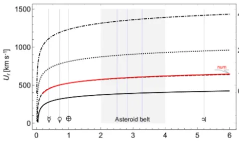
A comparison between the approximation ofUrusing Eq. (6) and a numerical solution of Eq. (4) is shown in Fig. 1. The solution shown in red and obtained forT =1 MK perfectly agrees with the analytical solution shown in dashed black. The Parker model thus predicts that the solar corona ex-pands radially outward at subsonic velocities close to the Sun (within the critical radius), and the coronal gas is gradually accelerated to supersonic velocities further out. Hereafter we also use an expression ofUswfor the magnitude of the solar wind velocity.
A more detailed analysis of the Parker model with the asymptotic solution of the flow velocity is presented by Sum-mers (1978). A two-fluid model of the solar wind is pre-sented by Summers (1982) as a hydrodynamic extension of the Parker model for the electron and the protons under the adiabatic law for each fluid type.
2.1.2 Spiral magnetic field
Using the angular velocity of the Sun,, the radial, po-lar, and azimuthal components of the solar wind velocity are given in the HG (heliographic) frame of reference as follows:
Ur=Usw, (7)
Uθ=0, (8)
Uφ= −rsinθ. (9)
A magnetic streamline satisfies the differential equation at a given polar angleθ,
1 rsinθ
dr dφ '
Ur Uφ
= − U
Figure 1.Radial solution of the solar windUrfor different
temper-atures in megakelvin (right frame ticks). Vertical lines indicate the position of the planets; the dark-shaded region covers the region of main belt asteroids of the solar system, where blue lines mark the position of mean motion resonances of asteroids with planet Jupiter.
We make use of a rough assumption that the flow speed is nearly constant over the critical radius beyond some distance r > rc. The field-line equation (Eq. 10) has then the solution as
r−r0= −Usw
(φ−φ0) . (11)
Here, the magnetic field line passes through the coordinate at(r0, θ, φ0). The IMF is obtained from the divergence-free condition of the Maxwell equations,
∇·B=0. (12) That is, using the assumption of spherical symmetry, the IMF is expressed as
Br=B0 r0
r 2
, (13)
Bθ=0, (14)
Bφ= −B0
r0 Usw
r0
r sinθ, (15)
whereB0is the radial component of the magnetic field at a reference radiusr0.
The transformation into the stationary frame (HGI, helio-graphic inertial) yields the same expression of the magnetic field as Eqs. (13)–(15).
Note that, due to a Galilean transformation, the electric field has a convective contribution in the polar directioneθ,
E= −U×B= −UswBφeθ. (16)
Realizations of the magnetic field lines in the Parker spiral model are shown for different (constant) solar wind speeds in Fig. 2. The angle between the magnetic field line and Earth’s orbit is about 45◦for a typical solar wind speed of
Figure 2.Streamlines in the Parker spiral model of interplanetary magnetic field around the Sun (a filled circle in yellow) in the helio-spheric ecliptic plane up to 5 astronomical units (au) under different conditions of the solar wind speed. The orbit of the Earth is marked by a blue curve at a radius of 1 au, that of Mars by a red curve (1.5 au), and that of Jupiter by a green curve (5 au).
400 km s−1and increases (becomes more radial) at a higher flow speed. Note that when considering the magnetohydro-dynamic (MHD) effect, the above discussion is valid outside the Alfvén radius at which the flow speed reaches the Alfvén speed,rA'50R=0.25 au, whereRis the solar radius.
We rewrite Eqs. (13)–(15) into a simpler form as Br=B0
r0 r
2
, (17)
Bφ= −r0B0 r0
r
cosϑ
Usw , (18)
where, again,B0=B (r0, θ, φ0)is the reference radial com-ponent of the magnetic field (Meyer-Vernet, 2012).
We note that in Eqs. (17)–(18) the latitudeϑ (measured from the Equator) is related to the polar angleθ (measured from the rotation axis) byθ=π−ϑ. By identifying or defin-ing the radial and tangential components as BR=Br and BT=Bφ, respectively, it is straightforward to transform the
Parker spiral field into its radial (R), tangential (T), and nor-mal (N) components as
BR=B0 r0
r 2
, (19)
BT= −r0B0 r0
r
sinθ
Usw . (20)
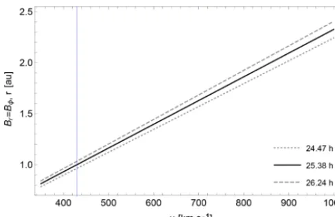
[image:4.612.45.285.65.209.2]Figure 3.Heliocentric distancerin astronomical units (au) at which the spiral angle of the interplanetary magnetic field reaches 45◦to the radial direction from the Sun (Br=Bφ). The curves are plotted as a function of the solar wind speed in units of km s−1for 3 differ-ent rotation rates, a period of 26.24 h (upper curve), 25.38 h (middle curve), and 24.47 h (lower curve). A typical value of the solar wind speed is 430 km s−1(shown by a vertical thin line).
2.1.3 Spiral angle
The distance to the surface on which an azimuthal angle of 45◦is realized (orBθ'Br) is approximately located at
r'Usw
sinθ. (21)
Using the rotation period of the Sun of 25.38 d (equivalent to an angular velocity of ω=2.865×10⁻⁶rad s−1) and the flow speedUsw'430 km s−1, the transition from the radially dominant to the azimuthally dominant magnetic field indeed happens aroundr=1 au. The transition distance is displayed as a function of the flow speed in Fig. 3 for three different solar rotation periods, 24.47, 25.38, and 26.24 d.
Alternatively, the Parker spiral model can be formulated in terms of the spiral angleψ:
tanψ=(r−R)sinθ
Usw . (22)
In this setting, the magnetic fieldBis, by using the unit vec-tors in the radial directioner and in the azimuthal direction eφ, given as
B=B0 r0
r 2
er−tanψeφ. (23)
In this formulation the magnitude of the magnetic field is estimated as
B=B0r0 r
2q
1+tan2ψ . (24)
2.1.4 Vector potential
The magnetic vector potentialAfor the Parker spiral mag-netic field under the Coulomb gauge∇·A=0 can analyti-cally be evaluated (Bieber et al., 1987). The vector potential has the following form:
Ar=
2a 3Usw
1−3x
2 −xln(1+x)
, (25)
Aθ=
2a 3Usw sinθ
x
1+x +ln(1+x)
, (26)
Aφ=
a
rsinθ(1−x) , (27) where x= |cosθ|. Equations (25)–(27) correspond to the IMF in the following expression:
Br= a r2
cosθ
|cosθ|, (28)
Bθ=0, (29)
Bφ= −
a Usw
sinθcosθ
|cosθ| . (30)
Here a is a free parameter proportional to the magnitude of the magnetic field in units of nT au2 (for example, a=
3.54 nT au2produces a magnetic field of 5 nT at 1 au). The polar component of the vector potential can be multiplied by a scalar functionf (θ )to improve the accuracy of the model asAθ→f (θ )Aθ.
Another formulation of the vector potential (again, under the Coulomb gauge) is to introduce a scalar potential as 8C= −2ar
3u
1−3x
2 −xln(1+x)
, (31)
which yields the following vector potential (Webb et al., 2010):
A=a
1− |cosθ| rsinθ eφ−
f (θ ) sinθ Usw
eθ
. (32) Of course, in both cases, Eqs. (25)–(27) and (32), the mag-netic field is obtained by the definition of the vector potential asB= ∇ ×A. The electrostatic potential for the convective electric fieldE= −U×B= −∇8is
8= −acosθ. (33)
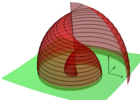
The magnetic field lines for the Parker spiral model are shown in Fig. 4. Black lines have been calculated by the in-tersection of the two surfaces of constant Euler potentialsαE, βE(Webb et al., 2010):
αE= −a|cosθ|, βE=φ+r
Usw
Figure 4.Magnetic field lines (black curves) in the Parker spiral model for different latitude anglesθfrom the rotation axis. Curves are defined as the intersection of the surfaces of the Euler potentials, αE=const.andβE=const., as presented by Webb et al. (2010).
Note that the spiral magnetic field lines are constructed with the ra-dial component from the Sun and the azimuthal component around the rotation axis and do not contain the polar component (in the direction toward the rotation axis and perpendicular to the radial di-rection). The spiral field lines have an axial component along the rotation axis, but this is due to the radial component of the spiral field line (in the sense of being away from the rotation axis).
the azimuthal component around the rotation axis and do not contain the polar component (in the direction toward the ro-tation axis and perpendicular to the radial direction) as in Eqs. (28)–(30). The Parker spiral field lines have an axial component along the rotation axis, but this is due to the radial component of the field line which has the axial component. For the sake of convenience one may set a value of unity to the variablesa,t,, andUswto provide the topology of the problem:αEdefines a cone (in green) that intersects a shell (in red) defined byβE. Intersection lines define the magnetic field lines of the Parker model.
2.2 Generalization of the Parker model
The Parker spiral model well approximates the mean and large-scale structure of the interplanetary magnetic field of our solar system. However, it fails to describe the three-dimensional geometry and evolution in time on various scales.
2.2.1 Latitudinal dependence
The Parker model does not recognize the sign reversal of the dipolar magnetic field over the Northern Hemisphere and the Southern Hemisphere; the divergence-free nature of the mag-netic field is not well represented. The hemispheric sign re-versal can be incorporated into the Parker model as follows (Webb et al., 2010):
B=af (θ )
r2
er−
rsinθ Ur
eφ
. (35)
Here, the constantaand functionf =f (θ )are given by a=σpB0r02, (36) f (θ )=1−2H (θ−π/2)= cosθ
|cosθ|, (37)
where σp= ±1 defines the polarity of the magnetic field in the Northern Hemisphere of the Sun, and f (θ ) is the Heaviside step function with the property f (θ )= +1 for 0< θ < π/2 andf (θ )= −1 forθ > π/2.
A more elaborated analytic model is proposed along with the Ulysses measurements over the solar polar regions (Zurbuchen et al., 1997; Forsyth et al., 2002). The three-dimensional model allows a nonzero field in the polar com-ponent and is expressed as
Br=B0 r0
r 2
, (38)
Bθ=
B0r02 Uswr
ωsinβFsin
φ+r
Usw
−φ0
, (39)
Bφ= −
B0r02 Uswr
sinθ−ω
cosβFsinθ+
sinβFcosθcos
φ+r
Usw
−φ0 , (40)
whereB0 is the radial component of the magnetic field at the source surface located at heliospheric distancer=r0,ω the differential rotation rate of the magnetic field line at foot points,βF(the Fisk angle) the polar angle at which a field line originating in the rotational pole crosses the source surface and is related to the angle between the solar magnetic dipole axis and the rotation axis, andφ0the heliographic longitude of the plane defined by the rotation and magnetic axes. The source magnetic field is defined atr=r0. The angleφ=φ0 occurs in the plane defined by the rotation axis and the mag-netic axis of the Sun. AngleβFis the polar angle where the field linepcrosses the source surface (from the heliographic pole). The angleβF can be calculated in the model by Fisk (1996) for a given orientationαFof the magnetic axisMand a given non-radial expansion. For the configuration discussed by Fisk (1996), the value ofβFis about 30◦.
A model of latitudinal dependence of the magnetic field is constructed by employing the method of separation of the variable for an axisymmetric magnetohydrodynamic outflow (Lima et al., 2001). The radial and the azimuthal components of the magnetic field are proposed as
Br=B0
r2 q
Bφ=λB0
sinθ r
r2 R2 s
−1 1−MA2
, (42)
whereis a free parameter,µis the ratio of the flow kinetic energy (or energy density, strictly speaking) in the equato-rial region to that in the polar region, and λ is the ratio of azimuthal to radial velocity (and also magnetic field) at the base of the wind.Rs is the radius of the star or the Sun.MA is the Alfvén Mach number of the flow. The polar compo-nent of the magnetic field is assumed to vanish due to the assumption of the axial symmetry around the rotation axis. 2.2.2 Poleward component
The IMF can have a nonzero polar (or latitudinal) compo-nent, e.g., from the solar dipolar field. Generalization of the Parker model to the nonzero polar component case (Bθ6=0)
is based on the analysis by Forsyth et al. (1996). LetφB be
the azimuthal angle that the projection of the IMF vector onto the R–T plane makes with the R axis in the right-handed sense andδBbe the meridional angle of the IMF to the R–T
plane. These angles are defined in terms of the magnetic field components (Forsyth et al., 1996):
tanφB=BT/BR,
sinδB=BN/B, (43)
whereB= q
BR2+BT2+BN2.
The azimuthal angle of the spiral fieldφPthat the tangent to the ideal Parker spiral magnetic field makes with the ra-dially outward direction at a position in interplanetary space specified by radial positionr and heliographic latitude δ is then given by
tanφP=Uφ−rcosδ
Ur
. (44)
On the assumption thatUφis small,φPturns out to be neg-ative. A magnetic field with a direction in agreement with the Parker spiral model will have eitherφB=φP in a region of outward polarity orφB=180◦+φPin a region of inward polarity field. In both regions the Parker model predicts that an ideal magnetic field has a meridional angleδB=0◦with
respect to the R–T plane. Therefore, up to the second order inBN the sine of the meridional angleδB according to the
second equation in Eq. (43) is given by
sinδB' BN q
BR2+BT2
. (45)
If we combine the first of Eq. (43) together with Eq. (45) and solve forBTandBNwe find up toO(BN3):
BT= −B0r0 r
2 Uφ−rcosδ Ur
, (46)
BN=B0 r0
r 2
v u u t1+ Uφ
−rcosδ2 U2
r
sinδB, (47)
where we substitutedBRbyBrin Eqs. (17)–(18),
BR=B0 r0
r 2
. (48)
Equations (46)–(48) provide a type of the Parker spiral mag-netic field with the generalization to a nonzero normal com-ponentBN6=0 parameterized byδandδB. ForδB=0◦and
ignoring the azimuthal component of the solar windUφ, the
model reproduces the Parker model, i.e., Eqs. (17)–(18):
BR=B0 r0
r 2
, (49)
BT= − r0
r
r0B0cosδ, (50)
BN=0. (51)
Another way of generalization is to use the power-law de-pendence using the power-law indexκ as a free parameter (Lhotka et al., 2016),
BR=BR0 r0
r 2
bR(t ) , (52)
BT=BT0 r0
r
bT(t ) , (53)
BN=BN0 r0
r κ
bR(t ) . (54)
Here,BR0,BT0, andBN0 are the mean magnetic field. bR, bT, and bN can be time-dependent such as the solar cycle (see Sect. 2.2.3). The power-law indexκ is a free parameter and determines the dependence ofBNon the inverse distance from the Sun 1/r.
2.2.3 Solar cycle dependence
the IMF as well. To include the time-dependent effect Kocifaj et al. (2006) suggests the following magnetic field model:
BR=B0r0 r
2 cos
π t 11[yr]+φ0
, (55)
BT= −B0r0 r
cosϑcos π t
11[yr]+φ0
. (56)
Here, ϑ is again latitude with θ=π−ϑ. Note that the transverse direction (with a unit vector eT) is constructed as eT=ωmag×eR, whereωmagis the magnetic axis of the Sun. If we assume that ωmag coincides with the rotation axis of the Sun,, then the relationBT= −Bφholds with
Bφ given in Eqs. (17)–(18). However, in comparison with
the second equation in Eqs. (17)–(18), the second equation in Eq. (35) differs by a factor r0/Ur in addition to the inclusion of the time-dependent terms. However, assuming solar wind speed Usw'450 km s−1 and solar rotation rate '2π/24.47 d−1, this factor becomes close to unity at r0=1 au.
2.2.4 Polarity and tilt angle
Two additional effects can further be incorporated into the IMF model, the polarityAmagand the tilt angleθtilt. The po-larity Amag is defined such that a case of Amag>0 corre-sponds to the magnetic fields pointing outward from the Sun in the Northern Hemisphere (the angle between the magnetic axis and the solar rotation axis is below 90◦), and a case of Amag<0 is in the opposite sense toAmag>0. Using the po-larityA, the Parker spiral magnetic field is given by the fol-lowing equation (Jokipii and Thomas, 1981):
B=Amag
r2 er−0eφ
×
1−2H
θ−
π
2 +θtiltsin
φ−r
Usw
, (57)
whereHis the Heaviside step function.0is defined as
0=rsinθ
Usw
. (58)
The polarityAmagis expressed in units of magnetic flux (see Eq. 23). An equivalent formulation of Eq. (57) is as follows (Kota and Jokippii, 1983):
B=Amag
r2
er−
rsinθ Usw
eφ
1−2H (θ−θ∗), (59)
cotθ∗= −tanθtiltsinφ∗, (60)
whereφ∗ is the azimuthal angle in the co-rotating frame at an angular speed of the solar rotation,
φ∗=φ+r
Usw
[image:8.612.306.549.70.178.2]. (61)
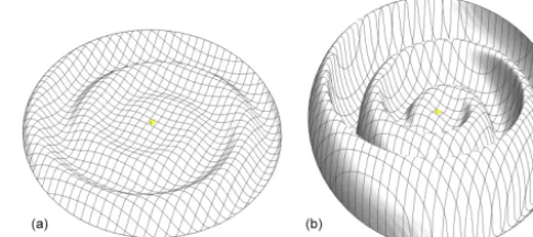
Figure 5.Shape of the “ballerina skirt” model of the heliocentric current sheet defined by cosθ∗=cosθ. Topology att=0 and for θt0=5◦(a)andθt0=30◦(b).
The tilt angleθtilt is larger at near solar maximum and smaller at near solar minimum (Thomas and Smith, 1981) and typically varies from 75◦at high level of solar activity to 10 down to 3◦during solar minimum activity. A model of tilt angle variation over a 22-year solar cycle was constructed by Jokipii and Thomas (1981) and Kota and Jokippii (1983) as follows:
θtilt=θt0+θt1cos 2π t
T
, (62)
whereθt0=20◦,θt1=10◦, andT =11 yr. The tilt angleθtilt is set to be at sunspot maximum att=0.
The wavy, flapping shape of the heliospheric current sheet is expressed by the equation for the polar angle as follows (Jokipii and Thomas, 1981):
θcs= π 2 +sin
−1
sinθtiltsin
φ−φ0+ r
Usw
, (63)
'π
2 +θtiltsin
φ−φ0+r
Usw
. (64)
The approximation in Eq. (64) is valid forθtilt1 rad (up to about 30◦).
A sketch of the topology of the heliospheric current sheet is shown in Fig. 5, where the magnetic field is discontinuous, i.e., for vanishingθ−θ∗=0 inH (θ−θ∗). For small values ofθtiltthe sheet is close to the plane defined in terms of the solar equator (left) while for larger values (θtilt=20◦) the wavy structure of the “ballerina skirt” is found to be much more pronounced.
The drift motion depends on the sign ofqAmag, a combi-nation of the electric charge of the particle and the polarity of the solar magnetic field. During the period ofqAmag>0, the time variation of the cosmic ray flux shows a flatter max-imum, while duringqAmag<0 the time variation of the cos-mic ray flux shows a shape maximum; see, e.g. Jokipii and Thomas (1981) or Kota and Jokippii (1983).
to the solar cycle dependence. The latitude-dependent mag-netic field model is expressed as follows:
Br=B0 r0
r 2
, (65)
Bθ=Br r Uswω
∗sinβ∗sinφ∗, (66)
Bφ=Br r Usw
ω∗sinβ∗cosθcosφ∗+
sinθ ω∗cosβ∗−+dω
∗
dθ sinβ ∗
sinθcosφ∗+
ω∗dβ ∗
dθ cosβ ∗
sinθcosφ∗
. (67)
Here
φ∗=φ−t+(r−r0)
Usw
+φ0. (68)
B0is again the radial component of the magnetic field at the reference radiusr0. The symbolβFis the angle (the Fisk an-gle) between the virtual magnetic axis (p axis) and the ro-tation axis of the Sun, and ωis the differential rotation rate of the Sun. Both the angle βF andωare generalized to the latitude-dependent case by introducing the transition func-tionFt(θ )in the following way:
β∗=βFFt(θ ), (69)
ω∗=ωFt(θ ). (70)
The transition function is constructed as follows (Burger et al., 2008):
Ft=
tanh[δpolθ] +tanh[δpol(θ−π )]
−tanh[δeq(θ−θb0)] 2
(71) for the northern high-latitude region (0≤θ < θb0),
Ft=0 (72)
for the equatorial or low-latitude region (θb0 ≤θ≤π−θb0), and
Ft=tanh[δpolθ] +tanh[δpol(θ−π )] −tanh[δeq(θ−π+θb0)]
2
(73) for the southern high-latitude region.θb0 is the equatorward-limit polar angle of the coronal hole (characterized by open field lines) and is between 60 and 80◦ from the solar ro-tation axis in Burger et al. (2008). The symbols δpol and δeq are the control parameters of the transition from the high-latitude magnetic fields (Fisk-type model) into the low-latitude fields (Parker-type model), e.g.,δpol=δeq=5.0 pro-posed by Burger et al. (2008). The magnetic field model in Eqs. (65)–(67) represents a natural extension of the Parker model in that the caseFt=1 reproduces the model proposed
by Zurbuchen et al. (1997) and the caseFt=0 reproduces the Parker model. The associated polar and azimuthal com-ponents of the flow velocity are
Uθ=r0ω∗sinβ∗sinφ, (74)
Uφ=r0
ω∗sinβ∗cosθcosφ+ω∗cosβ∗sinθ+
dω dθ sinβ
∗
sinθcosφ+
ω∗dβ ∗
dθ sinθcosφ
. (75)
The Fisk angleβF is related to the tile angle of the helio-spheric current sheetαFby Burger et al. (2008):
cos(αF+βF)=1− 1−cosθmm0 sin
2αF sin2θmm
, (76)
where θmm and θmm0 are the equatorward (low-latitude) boundary of the polar coronal hole on the level of photo-sphere source surface in heliomagnetic coordinates, respec-tively. The boundary angles are expressed in heliographic co-ordinates asθb=θmm−αFandθb0 =θmm0 −αF, respectively. The tilt anglesαFandβF and the boundary anglesθband θb0can be modeled in a time-dependent way when construct-ing the Fisk–Parker hybrid model (Burger et al., 2008) as a solar-cycle-dependent one: the time dependence of the tilt angleαFis modeled as
αF=αmin+ π
4 − αmin
2 h
1−cosπ 4T[yr]
i
(77)
for 0≤T[yr] ≤4 yr and αF=αmin+
π 4 −
αmin 2
h
1−cosπ
7(T[yr] −11) i
(78)
for 4< T ≤11yr, whereαmin=π/18 is an offset tilt angle. TimeT is measured in units of years after a solar minimum. The time dependence of the boundary angles is
θb=θb(min)
2 h
1+cosπ 4T[yr]
i
(79) θb0=θ
0 b(min)
2 h
1+cosπ 4T[yr]
i
(80)
for 0≤T ≤4yr and
θb=θb(min)
2 n
1+coshπ
7(T[yr] −11) io
(81) θb0=θ
0 b(min)
2 n
1+coshπ
7(T[yr] −11) io
(82)
3 Further models and effects 3.1 Magnetohydrodynamic models
The models of the solar wind and the interplanetary mag-netic field can be extended from kinematic or hydrodynamic treatments to magnetohydrodynamic (MHD) treatments. An overview of the MHD wind models is given by Tajima and Shibata (2002). Various magnetic effects are introduced in the MHD picture, e.g., the Alfvén velocity as a characteristic propagation speed (the Parker model, in contrast, recognizes the sound speed as a characteristic propagation speed) and the associated critical radius, collimation of the flow toward the rotation axis by magnetic pinching in the twisted field geometry.
3.1.1 One-dimensional treatment
An MHD model is proposed for an axisymmetric, one-dimensional, centrifugal-force-driven wind on the solar equatorial plane (Weber and Davis, 1967). Six variables are determined as a function of the radial distance (mass den-sity, ρ; radial and azimuthal components of flow speed,Ur andUφ; and that of the magnetic field,BrandBφ; and
pres-sure p) using six equations (continuity equation, magnetic flux conservation, force balance, induction equation, adia-batic pressure, and energy conservation) and six integral con-stants (mass flux, magnetic flux, angular velocity of the Sun, Alfvén radius, entropy, and total energy). The Alfvén radius is defined as the radius at which the flow velocity reaches the Alfvén velocity in the radial component,Ur=VA,r. At larger distances from the Sun, the solution is given asymptotically as
ρ∝r−2, (83)
Ur→U∞, (84)
Br∝r−2, (85)
Bφ∝r−1. (86)
The magnetic field becomes more azimuthal and thus twisted with increasing distance,Bφ/Br∝r.
The momentum balance equation by Parker (1958) is ex-tended to including the effect of magnetic field and Alfvén wave heating rate (Alazraki and Couturier, 1971; Belcher, 1971; Woolsey and Cranmer, 2014; Comi¸sel et al., 2015):
1 U
dU dr
U2−Uc2
= −Uc2 d
drlnB−c 2 s
d drlnT
+ QA
2ρ(U+VA)
−GM
r2 . (87)
Here QA denotes the Alfvén wave heating rate. Uc is the critical speed:
Uc2=c2s+WA
4ρ
3U+VA
U+VA , (88)
whereWAis the energy density of the Alfvén waves includ-ing the perpendicular fluctuation components of the flow ve-locityδU⊥and that of the magnetic fieldδB⊥,
WA=1
2ρδU 2 ⊥+
δB⊥2
2µ0. (89)
3.1.2 Two-dimensional treatment
In the two-dimensional picture, the energy conservation (the generalized Bernoulli equation) and the conservation law perpendicular to the magnetic field (the generalized Grad– Shafranov equation) are derived using the force balance equation among the advection of the flow itself (flow nonlin-earity such as steepening and eddies), the pressure gradient, the Lorentz force, and the gravitational attraction by the Sun, the mass flux conservation, the induction equation, and the adiabatic condition along the flow (Heinemann and Olbert, 1978; Sakurai, 1985; Lovelace et al., 1986). The generalized Grad–Shafranov equation cannot be solved analytically but needs to be solved numerically. It is found that the wind be-comes collimated toward the rotation axis of the Sun (or the star) by the magnetic pinching of the spiral or twisted field. In fact, any stationary, axisymmetric magnetized wind colli-mates toward the rotation axis at large distances (Heyvaerts and Norman, 1989).
It is useful to introduce the poloidal–toroidal expression of the magnetic field in the two-dimensional MHD treatment: Bp=∇×(aeφ)+Bφeφ, (90)
whereadenotes the magnetic stream function andeφis the
unit vector in the azimuthal direction around the rotation axis. The poloidal fieldsBp(the first term in Eq. 90) are ob-tained by a family of curves undera=const.We introduce the barred radius, which is the distance from the rotation axis, r=rsinθ. The flow velocity is decomposed by referring to the local magnetic field as
U=αm(a)
ρ B+r 2(a)e
φ, (91)
where the first term (denoted byUp) is the flow velocity com-ponent parallel to the magnetic field in the frame rotating with the angular velocity, and the second term (denoted byUφ) is perpendicular to the magnetic field. The toroidal
component of the magnetic field is determined by the angu-lar momentum conservation,
r
Uφ−
Bφ
µ0a
flow velocity expression in Eq. (91). The magnetic stream function needs to be determined for the flow velocity and the poloidal component of the magnetic field. The magnetic stream function is numerically evaluated from the momen-tum equation (or force balance) perpendicular to the mag-netic field by solving the following equation (Sakurai, 1985): ∇·
α2 m ρ −
1 µ0
∇a
r2
=ρ
E0− 1
γp−1 p ρ
K0 K +r
20
+B
2 p ρ αmα
0 m+D
D
µ0
2r2αmα0m−αm22(r2A)0
−α2m0r2A−rA i
, (93)
where D= µ0ρ r
2 A−r2
r2(µ0ραm2−ρ)
(94) and the prime (·)0 denotes the differentiation with re-spect to the magnetic stream function, d/da. Equation (93) is the generalized Grad–Shafranov equation for the two-dimensional centrifugally driven wind. The densityρfollows the Bernoulli equation:
Up2 2 +
1
2(Uφ−r) 2+ γp
γp−1 p ρ−
GM· r −
2r2
2 =E(a) (95) under the polytropic or adiabatic equation of state
p=K(a)ργp. (96)
In the two-dimensional MHD treatment of the flow, the wind becomes collimated toward the rotation axis by the pinch of toroidal fields (Sakurai, 1985), causing a nonzero poleward (northward or southward) component of the magnetic field. 3.2 More ingredients
Solar wind models can further be improved by considering turbulent diffusion and pickup ions.
3.2.1 Turbulent diffusion
Turbulence on smaller spatial scales serves as an energy sink to large-scale mean fields, which leads to the notion of turbu-lent diffusion (mean-field electrodynamics). To see this more clearly, one may decompose the magnetic field into a large-scale mean fieldB0and a fluctuating fieldδB(with the zero mean value), as well as the flow velocity:
B=B0+δB, (97)
U=U0+δU. (98)
The induction equation for the large-scale magnetic field has then the frozen-in term for the large-scale fieldsB0andU0 and the electromotive force termEem:
∂B0
∂t =∇×(U0×B0)+∇×Eem. (99)
The electromotive force is an averaged electric field coming from the coupling of the flow velocity fluctuations with the fluctuating magnetic field by the cross product:
Eem= hδU×δBi. (100)
A widely used model in the mean-field electrodynamics is that the electromotive force depends on the large-scale quan-tities such as the large-scale magnetic field, the curl of the large-scale magnetic field, and the curl of the large-scale flow velocity. By introducing the proper transport coefficientsαt, βt, andγt, the electromotive force is modeled as
Emodel=αtB0−βt∇×B0+γt∇×U0. (101) After some algebra using Eqs. (99) and (101), one identi-fies that the termβt∇×B0becomes nothing other than the diffusion term for the large-scale magnetic field (under the condition that the coefficientβtis not negative):
∂B0
∂t =∇×(U0×B0)+∇×(αtB0)+βt∇ 2B
0
+∇×(γt∇×U0) . (102)
The terms withαtandγtin turn may amplify the large-scale magnetic field when the coefficients are in favor of field am-plification (dynamo mechanism). The transport coefficients are theoretically estimated as follows:
αt=Cατ (−hkin+hcur), (103)
βt=Cβτ ekin+emag, (104)
γt=Cγτ hcrs, (105)
whereCα,Cβ, andCγ are dimensionless scalar factors and
are estimated as (Yoshizawa, 1998)
Cα'0.02, (106)
Cβ'0.05, (107)
Cγ '0.04. (108)
The symbolτ denotes the turbulent correlation time length, andhanderepresent the helicity and the energy quantities: hkinthe kinetic helicity density,hcurthe current helicity den-sity,hcrsthe cross helicity density,ekinthe turbulent kinetic energy density, andemagthe turbulent magnetic energy den-sity. The helicity density quantities and the energy density quantities are defined for the fluctuating field:
hkin= hδU·(∇×δU)i, (109)
hcur= 1
µ0ρ0
hδB·(∇×δB)i, (110)
hcrs=√1
µ0ρ0
hδU·δBi, (111)
ekin=1
2h|δU|
emag= 1 2µ0ρ0
h|δB|2i. (113)
Note that different definitions are possible for the helicity and energy density quantities. In the definition above (Eqs. 109– 113) the fluctuating magnetic field is converted into the ve-locity dimension such as δB/√µ0ρ0, and the energy den-sity is represented as that per unit mass. The correlation time lengthτ can in the simplest case be modeled or represented by the eddy turnover time,
τed= `
δU =
ekin+emag
ε , (114)
whereεis the dissipation rate which needs to be obtained by solving an equation in the similar fashion to the turbulence energy (Yokoi et al., 2008). The estimate of timescale can be extended by including the Alfvén time effect into a syn-thesized timescale τs in the additive sense in the frequency domain as
1 τs =
1 τed+χ
1
τA, (115)
whereτAdenotes the Alfvén time
τA= ` VA =
|ekin+emag|2
εVA2 , (116)
with the length scale`and the Alfvén speedVA. The symbol χis the weight factor for the Alfvén time and is estimated to be of the order 102in the solar wind application (Yokoi et al., 2008). A more rigorous treatment is to solve two sets of equa-tions, one for the large-scale mean fields and the other for the small-scale turbulent fields. This task can be achieved either analytically using the two-scale direct interaction approxi-mation (Yokoi, 2006; Yokoi and Hamba, 2007; Yokoi et al., 2008) or numerically (Usmanov et al., 2012, 2014, 2016). 3.2.2 Pickup ions
Pickup ions from interstellar neutral hydrogen atoms are one of the ingredients to the solar wind and contribute to addi-tional mass of the plasma, which results in deceleration of the solar wind expansion and in increase in the plasma temper-ature. Pickup ions originate in (1) charge exchange with the solar wind protons and (2) photoionization by the solar ra-diation. Steady-state MHD equations for the wind including pickup ions are introduced by Isenberg (1986) and Whang (1998) and are numerically implemented to simulation stud-ies for a three-component fluid (thermal protons, electrons, pickup protons) by Usmanov and Goldstein (2006) and Us-manov et al. (2014) and for a four-component fluid by adding interstellar hydrogen (Usmanov et al., 2016).
The continuity equation in the one-fluid sense (mixture of electrons, solar wind protons, and pickup ions of interstel-lar origin) has a contribution from the photoionization as a
source term and is written for the steady state as (Whang, 1998)
∇·(ρU)=mpqph, (117) whereρandUdenote the mass density and the flow velocity in the one-fluid sense,mpthe proton mass, andqphthe pickup ion production rate by the photoionization process,
qph=ν0 r02
r !
nnt. (118)
Hereν0=0.9×10⁻⁷s−1is the photoionization rate per hy-drogen atom at the Earth orbit distance as reference r0=
1 au, andnnt is the number density of neutral hydrogen (of interstellar origin). The one-fluid momentum equation in the steady state is approximated into (by neglecting higher-order terms) (Whang, 1998)
ρU·U+∇P−ρ∇
GM r
− 1
µ0(∇×B)×B=
−(qex+qph)mpU. (119) Hereqexis the pickup ion production rate by the charge ex-change process,
qex=σexnswnntU, (120)
whereσex is the cross section of charge exchange between a hydrogen atom and the solar wind protons, andnswis the number density of solar wind protons.
3.3 Stellar wind and interstellar space
Various outflow models have been proposed for the stellar wind. For example, a wind model is constructed and numeri-cally studied for the thermally driven hydrodynamic outflow from low-mass stars (Johnstone et al., 2015). A dead zone due to the magnetic dipole field effect can arise in the equa-torial region (Keppens and Goedlbloed, 1999). A model is also constructed for the stellar winds around asymptotic giant branch (AGB) stars with dust grains by employing the MHD equation for the stellar wind plasma and the Euler equation for the dust grains under the gravity, the radiation pressure, and the drag force (Thirumalai and Heyl, 2010), showing the possibility of a stellar wind driven by dust grains. The mass-loss rate is observationally studied via stellar winds for sub-luminous stars (Krtiˇcka et al., 2016), in which the following flow velocity model is used for fitting with three parameters U1,U2, andγsw:
U= "
U1
1−Rs
r
+U2
1−Rs
r 2#
( 1−exp
" γsw
1− r
Rs 2#)
whereRsis the stellar radius.
Stellar winds can be detected by the spectroscopic inves-tigation. A line spectrum becomes distorted to blue-shifted absorption and red-shifted emission by the retarding stellar wind (away from the observer), known as the P Cygni pro-file. One type of the stellar wind models is the Lucy model (Lucy, 1971):
U=Ut
1−(1−asw)Rs
r −asw R2s
r2 1/2
, (122)
where asw is a free parameter with −1< asw<1. Equa-tion (122) satisfies the condiEqua-tions of zero speed at the stel-lar surface (U=0 at r=Rs) and asymptotic behavior at very large distances from the star (U→Ut as r→ ∞). Ut is the terminal flow velocity. The flow speed increases monotonously as a function of the radius,U >0 and ddUr >0. The other type is a variant of the Lucy model (Kudritzki and Puls, 2000):
U Ut
=
1−bsw Rs
r βsw
, (123)
where the constantbswis the flow velocity at the inner bound-ary of the stellar wind. An even more simplified expression is (Lamers, 1998)
U Ut
=
1−Rs
r βsw
, (124)
whereUt is the asymptotic, termination flow speed. βsw is a free parameter and is empirically chosen as 0.5≤βsw≤4 (Sapar et al., 2003).
4 Summary and conclusions
There is an increasing amount of models for the interplane-tary magnetic field. Starting with the Parker model, the mag-netic field model can be extended to include the latitudinal dependence, the poleward component, the time dependence, and the polarity and tilt effect even in the analytic or semi-analytic treatment. Which model to choose would depend on the application, e.g., if the solar cycle is to be included or not, or if the latitudinal dependence is to be or not. In the tem-poral sense, cosmic ray diffusion has the shortest timescale, about 13 h for relativistic particles nearly at the speed of light to travel over 100 au distance in the heliosphere. In contrast, plasma turbulence evolves together with the solar wind, and the timescale is intermediate, being of the order or days; i.e., the solar wind travel time from the Sun to the Earth orbit, 1 au, is about 100 h or roughly 4 d. Charged dust motions and modulation of the cosmic ray flux in the heliosphere evolve on the longest timescale among the three applications, of the order of of years (secular variation of the orbital parameters).
The accuracy or the uncertainty of the reviewed mod-els needs to be verified using in situ magnetic field mea-surements from the previous, current, and upcoming space-craft missions. Above all, the magnetic field in the inner heliosphere will be extensively studied with Parker Solar Probe, BepiColombo (in particular, the cruise-phase mea-surements), and Solar Orbiter.
It is interesting to note that the analytic expression is also available for the coronal magnetic field (during the solar min-imum) and the local interstellar magnetic field surrounding the heliosphere. Hence, naively speaking, one may expect to construct a more complete model of the magnetic field from the Sun to the local interstellar medium. Such a model, once smoothly and rationally connected from one region to another, enables one to improve the accuracy of theoretical studies on plasma turbulence evolution, charged dust mo-tions, and diffusion of cosmic ray and energetic particles.
It is also worth noting the limits of the models. First, the magnetic fields are highly irregular in structure in the so-lar corona and at the soso-lar surface. At some distance suf-ficiently close to the Sun, the interplanetary magnetic field should smoothly be connected to the coronal magnetic field. Second, the outer heliosphere has the termination shock and the heliopause, which are not included in the models in this review. Third, the solar variability includes not only the 11-year sunspot number variation or the 22-11-year magnetic struc-ture variation, but also modulations of the solar cycle on long timescales such as 100 or even 1000 years.
Data availability. No data sets were used in this article.
Author contributions. This article has been prepared by both au-thors in equal parts.
Competing interests. The authors declare that they have no conflict of interest.
Acknowledgements. This work is financially supported by the Aus-trian Space Applications Programme FFG ASAP-12 SOPHIE at the Austrian Research Promotion Agency under contract 853994 and the Austrian Science Funds (FWF) under contract P30542-N27.
References
Alazraki, G. and Couturier, P.: Solar wind acceleration caused by the gradient of Alfvén wave pressure, Astron. Astrophys., 13, 380–389, 1971.
Alfvén, H.: On the theory of comet tails, Tellus, 9, 92–96, https://doi.org/10.3402/tellusa.v9i1.9064, 1957.
Banaszkiewicz, M., Axford, W. I., and McKenzie, J. F.: An analytic solar magnetic field model, Astron. Astrophys., 337, 940–944, 1998.
Belcher, J. W.: Alfvénic wave pressures and the solar wind, Astro-phys. J., 168, 509, https://doi.org/10.1086/151105, 1971. Benkhoff, J., van Casteren, J., Hayakawa, H., Fujimoto, M., Laakso,
H., Novara, M., Ferri, P., Middleton, H. R., and Ziethe, R.: BepiColombo – Comprehensive exploration of Mercury: Mis-sion overview and science goals, Planet. Space Sci., 58, 2–20, https://doi.org/10.1016/j.pss.2009.09.020, 2010.
Bieber, J. W., Evenson, P. A., and Matthaeus, W. H.: Mag-netic helicity of the Parker field, Astrophys. J., 315, 700–705, https://doi.org/10.1086/165171, 1987.
Biermann, L.: Kometenschweife und solare Korpuskularstrahlung, Z. Astrophys., 29, 274–286, 1951.
Biermann, L.: Solar corpuscular radiation and the interplanetary gas, Observatory, 77, 109–110, 1957.
Bruno, R. and Carbone, V.: The solar wind as a tur-bulence laboratory, Living Rev. Sol. Phys., 10, 2–208, https://doi.org/10.12942/lrsp-2013-2, 2013.
Burger, R. A., Krüger, T. P. J., Hitge, M., and Engelbrecht, N. E.: A Fisk-Parker hybrid heliospheric magnetic field with a solar-cycle dependence, Astrophys. J., 674, 511–519, https://doi.org/10.1086/525039, 2008.
Coleman Jr., P. J.: Turbulence, viscosity, and dissipation in the solar-wind plasma, Astrophys. J., 153, 371–388, https://doi.org/10.1086/149674, 1968.
Comi¸sel, H., Motschmann, U., Büchner, J., Narita, Y., and Nariyuki, Y.: Ion-scale turbulence in the inner heliosphere: Radial de-pendence, Astrophys. J., 812, 175, https://doi.org/10.1088/0004-637X/812/2/175, 2015.
Czechowski, A. and Mann, I.: Formation and Acceleration of Nano Dust in the Inner Heliosphere, Astrophys. J., 714, 89–99, https://doi.org/10.1088/0004-637X/714/1/89, 2010.
Duldig, M. L.: Australian cosmic ray modulation research, Publ. Asron. Soc. Australia, 18, 12–40, 2001.
Fisk, L. A.: Motion of the footpoints of heliospheric magnetic field lines at the Sun: Implications for recurrent energetic par-ticle events at high heliographic latitudes, J. Geophys. Res., 101, 15547–15554, https://doi.org/10.1029/96JA01005, 1996. Forsyth, R. J., Balogh, A., Horbury, T. S., Erdoes, G., Smith, E. J.,
and Burton, M. E.: The heliospheric magnetic field at solar min-imum: ULYSSES observations from pole to pole, Astron. Astro-phys., 316, 287–295, 1996.
Forsyth, R. J., Balogh, A., and Smith, E. J.: The under-lying direction of the heliospheric magnetic field through the Ulysses first orbit, J. Geophys. Res.-Space, 107, 1405, https://doi.org/10.1029/2001JA005056, 2002.
Fox, N. J., Velli, M. C., Bale, S. D., Decker, R., Driesman, A., Howard, R. A., Kasper, J. C., Kinnison, J., Kusterer, M., Lario, D., Lockwood, M. K., McComas, D. J., Raouafi, N. E., and Szabo, A.: The Solar Probe Plus mission:
Hu-manity’s first visit to our star, Space Sci. Rev., 204, 7–48, https://doi.org/10.1007/s11214-015-0211-6, 2016.
Grün, E., Gustafson, B., Mann, I., Baguhl, M., Morfill, G. E., Staubach, P., Taylor, A., and Zook, H. A.: Interstellar dust in the heliosphere, Astron. Astrophys., 286, 915–924, 1994.
Heinemann, M. and Olbert, S. J.: Axisymmetric ideal MHD stellar wind flow, J. Geophys. Res., 83, 2457–2460, https://doi.org/10.1029/JA083iA06p02457, 1978.
Henry, Z. W., Nykyri, K., Moore, T. W., Dimmock, A. P., and Ma, X.: On the Dawn-Dusk Asymmetry of the Kelvin-Helmholtz In-stability Between 2007 and 2013, J. Geophys. Res.-Space, 122, 11888–11900, https://doi.org/10.1002/2017JA024548, 2017. Heyvaerts, J. and Norman, C.: The collimation of
magnetized winds, Astrophys. J., 347, 1055–1081, https://doi.org/10.1086/168195, 1989.
Isavnin, A.: FRiED: A novel three-dimensional model of coronal mass ejections, Astrophys. J., 833, 267, https://doi.org/10.3847/1538-4357/833/2/267, 2017.
Isenberg, P. A.: Interaction of the solar wind with interstellar neutral hydrogen: Three-fluid model, J. Geophys. Res., 91, 9965–9972, https://doi.org/10.1029/JA091iA09p09965, 1986.
Isenberg, P. A. and Jokipii, J. R.: Gradient and curvature drifts in magnetic fields with arbitrary spatial variation, Astrophys. J., 234, 746–752, https://doi.org/10.1086/157551, 1979.
Jokipii, J. R. and Thomas, B.: Effects of drift on the trans-port of cosmic rays, IV – Modulation by a wavy in-terplanetary current sheet, Astrophys. J., 243, 1115–1122, https://doi.org/10.1086/158675, 1981.
Johnstone, C. P., Güdel, M., Lüftinger, T., Toth, G., and Brott, I.: Stellar winds on the main-sequence, I. Wind model, Astron. Astrophys., 577, A27, https://10.1051/0004-6361/201425300, 2015.
Katsiaris, G. A. and Psillakis, Z. M.: An analytic model of the Earth’s magnetosphere, Astrophys. Space Sci., 132, 165–175, 1987.
Keppens, R. and Goedlbloed, J. P.: Numerical simulations of stel-lar winds: polytropic models, Astron. Astrophys., 343, 251–260, 1999.
Kocifaj, M., Klaˇcka, J., and Horvath, H.: Temperature-influenced dynamics of small dust particles, Mon. Not. Royal As-tron. Soc., 370, 1876–1884, https://doi.org/10.1111/j.1365-2966.2006.10612.x, 2006.
Kohlhase, C. E. and Penzo, P. A.: Voyager mis-sion description, Space Sci. Rev., 21, 77–101, https://doi.org/10.1007/BF00200846, 1977.
Kota, J. and Jokipii, J. R.: Effects of drift on the transport of cosmic rays, VI – A three-dimensional model including diffusion, As-trophys. J., 265, 573–581, https://doi.org/10.1086/160701, 1983. Kóta, J. and Jokipii, J. R.: 3-D modeling of cosmic-ray transport in the heliosphere: toward solar maximum, Adv. Space Res., 27, 529–534, 2001a.
Kóta, J. and Jokipii, J. R.: The anisotropies of galactic cosmic rays: 3-dimensional modeling, Adv. Space Sci., 27, 607–612, 2001b. Krtiˇcka, J., Kubát, J., and Krtiˇcková, I.: Stellar wind
mod-els of subluminous hot stars, Astron. Astrophys., 593, A101, https://doi.org/10.1051/0004-6361/201628433, 2016.
Lamers, H. J. G. L. M.: Observations of stellar winds, Astrophys. Space Sci., 260, 63–80, 1998.
Lima, J. J. G., Priest, E. R., and Tsinganos, K.: An analytical MHD wind model with latitudinal dependences obtained using separation of the variables, Astron. Astrophys., 371, 240–249, https://doi.org/10.1051/0004-6361:20010353, 2001.
Lhotka, C., Bourdin, P., and Narita, Y.: Charged dust grain dynamics subject to solar wind, Poynting-Robertson drag, and the interplanetary magnetic field, Astrophys. J., 828, 10, https://doi.org/10.3847/0004-637X/828/1/10, 2016.
Lovelace, R. V. E., Mehanian, C., Mobarry, C. M., and Sulkanen, M. E.: Theory of axisymmetric magnetohydro-dynamic flows – Disks, Astrophys. J. Suppl. 62, 1–37, https://doi.org/10.1086/191132, 1986.
Lucy, L. B.: The formation of resonance lines in extended and expanding atmospheres, Astrophys. J., 163, 95–110, https://doi.org/10.1086/150748, 1971.
Mann, I., Murad, E., and Czechowski, A.: Nanoparticles in the inner solar system, Planet. Space Sci., 55, 1000–1009, https://doi.org/10.1016/j.pss.2006.11.015, 2007.
Mann, I., Meyer-Vernet, N., and Czechowski, A.: Dust in the planetary system: Dust interactions in space plasmas of the solar system, Phys. Rep., 536, 1–39, https://doi.org/10.1016/j.physrep.2013.11.001, 2014.
Matthaeus, W. H., Goldstein, M. L., and Smith, C.: Evaluation of magnetic helicity in homogeneous turbulence, Phys. Rev. Lett., 48, 1256–1259, https://doi.org/10.1103/PhysRevLett.48.1256, 1982.
Meyer-Vernet, N.: Basics of the Solar Wind, Cambridge University Press, Cambridge, 2012.
Miyahara, H., Yokoyama, Y., and Yamaguchi, Y. T.: Influence of the Schwabe/Hale solar cycles on climate change during the Maun-der Minimum, Proc. IAU Symposium, 264, in: Solar and Stellar Variability: Impact on Earth and Planets, edited by: Kosovichev, A. G., Andrei, A. H., and Rozelot, J.-P., International Astronom-ical Union, https://doi.org/10.1017/S1743921309993048, 2010. Müller, D., Marsden, R. G., StCyr, O. C., and Gilbert, H. R.: Solar
Orbiter: Exploring the Sun-heliosphere connection, Sol. Phys., 285, 25–70, https://doi.org/10.1007/s11207-012-0085-7, 2013. Ness, N. F. and Wilcox, J. M.: Solar origin of the
inter-planetary magnetic field, Phys. Rev. Lett., 13, 461–464, https://doi.org/10.1103/PhysRevLett.13.461, 1964.
Ness, N. F., Scearce, C. S., and Seek, J. B.: Initial results of the imp 1 magnetic field experiment, J. Geophys. Res., 69, 3531–3569, https://doi.org/10.1029/JZ069i017p03531, 1964.
Owens, M. and Forsyth, R. J.: The heliospheric magnetic field, Living Rev. Solar Phys., 10, 5–52, https://doi.org/10.12942/lrsp-2013-5, 2013.
Parker, E. N.: Dynamics of the interplanetary gas and magnetic fields, Astrophys. J., 128, 664, https://doi.org/10.1086/146579, 1958.
Parker, E. N.: The passage of energetic charged particles through interplanetary space, Planet. Space Sci., 13, 9–49, 1965. Petrosyan, A., Balogh, A., Goldstein, M. L., Léorat, J., Marsch,
E., Petrovay, K., Roberts, B., von Steiger, R., and Vial, J. C.: Turbulence in the solar atmosphere and solar wind, Space Sci. Rev., 156, 135–238, https://doi.org/10.1007/s11214-010-9694-3, 2010.
Porsche, H.: HELIOS mission: Mission objectives, mission verifi-cation, selected results, ESA, The Solar System and Its Explo-ration, 43–50, 1981.
Potgieter, M. S.: Solar modulations of cosmic rays, Living Rev. Sol. Phys., 10, 3–66, https://doi.org/10.12942/lrsp-2013-3, 2013. Röken, C., Kleimann, J., and Fichtner, H.: An exact
ana-lytical solution for the interstellar magnetic field in the vicinity of the heliosphere, Astrophys. J., 805, 173–186, https://doi.org/10.1088/0004-637X/805/2/173, 2015.
Sakurai, T.: Magnetic stellar winds: a 2-D generalization of the Weber-Davis model, Astron. Astrophys., 152, 121–129, 1985. Sapar, A., Sapar, L., and Poolamäe, R.: Analytical solutions for
sat-urated P cygni type profiles II: general case, Astrophys. Space Sci., 286, 333–345, https://doi.org/10.1023/A:1026374800760, 2003.
Schwenn, R. and Marsch, E. (Eds.): Physics of the Inner He-liosphere, 1: Large Scale Phenomena, Springer-Verlag, Berlin-Heidelberg, 1990.
Schwenn, R. and Marsch, E. (Eds.): Physics of the Inner He-liosphere, 2: Particles, Waves and Turbulence, Springer-Verlag, Berlin-Heidelberg, 1991.
Shukla, P. K. and Mamun, A. A.: Introduction to Dusty Plasma Physics, Institute of Physics, Series in Plasma Physics ISBN:978-075030653X, CRC Press, 2001.
Stone, E. C.: The Voyager missions to the outer system, Space Sci. Rev., 21, 75–75, https://doi.org/10.1007/BF00200845, 1977. Stone, E. C.: The Voyager Mission – Encounters
with Saturn, J. Geophys. Res., 88, 8639–8642 https://doi.or/10.1029/JA088iA11p08639, 1983.
Summers, D.: Fluid models of the solar wind, J. Inst. Maths. Ap-plics, 22, 71–87, 1978.
Summers, D.: On the two-fluid polytropic solar wind model, Astro-phys. J., 257, 881–886, https://doi.org/10.1086/160037, 1982. Tajima, T. and Shibata, K.: Plasma Astrophysics, Westview Press,
Boulder, Colorado, 2002.
Thirumalai, A. and Heyl, J. S.: A hybrid steady-state mag-netohydrodynamic dust-driven stellar wind model for AGB stars, Mon. Not. R. Astron. Soc., 409, 1669–1681 https://doi.org/10.1111/j.1365-2966.2010.17414.x, 2010. Thomas, B. T. and Smith, E. J.: The structure and dynamics of the
heliospheric current sheet, J. Geophys. Res., 86, 11105–11110, https://doi.org/10.1029/JA086iA13p11105, 1981.
Tsyganenko, N. A.: Quantitative models of the magnetospheric magnetic field – Methods and results, Space Sci. Rev., 54, 75– 186, https://doi.org/10.1007/BF00168021, 1990.
Tsyganenko, N. A.: Modeling the Earth’s magnetospheric magnetic field confined within a realistic magnetopause, J. Geophys. Res., 100, 5599–5612, https://doi.org/10.1029/94JA03193, 1995. Tsyganenko, N. A. and Sitnov, M. I.: Magnetospheric
configurations from a high-resolution data-based mag-netic field model, J. Geophys. Res., 112, A06225, https://doi.org/10.1029/2007JA012260, 2007.
Tu, C.-Y. and Marsch, E.: MHD structures, waves and turbulence in the solar wind: Observations and theories, Space Sci. Rev., 73, 1–210, https://doi.org/10.1007/BF00748891, 1995.
Usmanov, A. V., Matthaeus, W. H., Breech, B. A., and Gold-stein, M. L.: Solar wind modeling with turbulence transport and heating, Astrophys. J., 727, 84, https://doi.org/10.1088/0004-637X/727/2/84, 2011.
Usmanov, A. V., Goldstein, M. L., and Matthaeus, W. H.: Three-dimensional magnetohydrodynamic modeling of the solar wind including pickup protons and turbulence transport, Astrophys. J., 764, 40, https://doi.org/10.1088/0004-637X/754/1/40, 2012. Usmanov, A. V., Goldstein, M. L. and Matthaeus, W. H.:
Three-fluid, three-dimensional magnetohydrodynamic solar wind model with eddy viscosity and turbulent resistivity, Astrophys. J., 788, 25–43, https://doi.org/10.1088/0004-637X/788/1/43, 2014. Usmanov, A. V., Goldstein, M. L., and Matthaeus, W. H.: A four-fluid MHD model of the solar wind/interstellar medium inter-action with turbulence transport and pickup protons as sepa-rate fluid, Astrophys. J., 820, 2–17, https://doi.org/10.3847/0004-637X/820/1/17, 2016.
Weber, E. J. and Davis Jr., L.: The angular momen-tum of the solar wind, Astrophys. J., 148, 217–227, https://doi.org/10.1086/149138, 1967.
Webb, G. M., Hu, Q., Dasgupta, B., and Zank, G. P.: Homo-topy formulas for the magnetic vector potential and magnetic helicity: The Parker spiral interplanetary magnetic field and magnetic flux ropes, J. Geophys. Res.-Space, 115, A10112, https://doi.org/10.1029/2010JA015513, 2010.
Whang, Y. C.: Solar wind in distant heliosphere, J. Geophys. Res., 103, 17419–17428, https://doi.org/10.1029/98JA01524, 1998. Wenzel, K.-P. and Smith, E. J.: Ulysses: A voyage
above the Sun’s poles, Europhys. News, 22, 203–205, https://doi.org/10.1051/epn/19912211203, 1991.
Wenzel, K. P., Marsden, R. G., Page, D. E., and Smith, E. J.: The ULYSSES mission, Astron. Astrophys. Suppl., 92, 207–219, 1992.
Wilcox, J. M.: The interplanetary magnetic field. Solar ori-gin and terrestrial effects, Space Sci. Rev., 8, 258–328, https://doi.org/10.1007/BF00227565, 1968.
Wilcox, J. M. and Ness, N. F.: Quasi-stationary corotating structure in the interplanetary medium, J. Geophys. Res., 70, 5793–5805, https://doi.org/10.1029/JZ070i023p05793, 1965.
Woolsey, L. N. and Cranmer, S. R.: Turbulence-driven coronal heating and improvements to empirical forecasting of the so-lar wind, Astrophys. J., 787, 160, https://doi.org/10.1088/0004-637X/787/2/160, 2014.
Yokoi, N.: Modeling of the turbulent magnetohydrodynamic residual-energy equation using a statistical theory, Phys. Plas-mas, 13, 062306, https://doi.org/10.1063/1.2209232, 2006. Yokoi, N.: Modeling the turbulent cross-helicity evolution:
produc-tion, dissipaproduc-tion, and transport rates, J. Turbulence, 12, N27, https://doi.org/10.1080/14685248.2011.590495, 2011.
Yokoi, N. and Hamba, F.: An application of the turbulent magneto-hydrodynamic residual-energy equation model to the solar wind, Phys. Plasmas, 14, 112904, https://doi.org/10.1063/1.2792337, 2007.
Yokoi, N., Rubinstein, R., Yoshizawa, A., and Hamba, F.: A turbu-lence model for magnetohydrodynamic plasmas, J. Turbuturbu-lence, 9, 1–25, https://10.1080/14685240802433057, 2008.
Yoshizawa, A.: Hydrodynamic and Magnetohydrodynamic Turbu-lent Flows: Modelling and Statistical Theory, Kluwer Academic Publishers, Dordrecht, 1998.