Development and Testing of a Collision Avoidance Braking System for an Autonomous Vehicle



Abstract: The article describes the main development and testing aspects of an emergency braking function for an autonomous vehicle. The purpose of this function is to prevent the vehicle from collisions with obstacles, either stationary or moving. An algorithm is proposed to calculate deceleration for the automated braking, which takes into account the distance to the obstacle and velocities of both the vehicle and the obstacle. In addition, the algorithm adapts to deviations from the required deceleration, which are inevitable in the real-world practice due to external and internal disturbances and unaccounted dynamics of the vehicle and its systems. The algorithm was implemented as a part of the vehicle’s mathematical model. Simulations were conducted, which allowed to verify algorithm’s operability and tentatively select the system parameters providing satisfactory braking performance of the vehicle. The braking function elaborated by means of modeling then was connected to the solenoid braking controller of the experimental autonomous vehicle using a real-time prototyping technology. In order to estimate operability and calibrate parameters of the function, outdoor experiments were conducted at a test track. A good consistency was observed between the test results and simulation results. The test results have proven correct operation of the emergency braking function, acceptable braking performance of the vehicle provided by this function, and its capability of preventing collisions.

Keywords: automated braking, autonomous vehicle, control system, simulations, testing.

I. INTRODUCTION

This article offers a description of a research and development project in the field of vehicle driving automation. The outcome of this work is supposed to be an experimental autonomous vehicle of a special purpose explained below. Specifically, the article presents the part of the project, in which an emergency braking function for the said vehicle was elaborated, implemented and tested. Necessity of this function for autonomous vehicles is obvious, which entails a substantial number of published works focused on research and development thereof [1]-[12]. Besides, the automated emergency braking function is currently making its way into the domain of conventional vehicles becoming a part of active safety systems [1].

Revised Manuscript Received on September 05, 2019.

Ilya Aleksandrovich Kulikov*, Federal State Unitary Enterprise Central Scientific Research Automobile and Automotive Institute "NAMI" (FSUE «NAMI»), Moscow, Russia.

Ivan Alekseevich Ulchenko, Federal State Unitary Enterprise Central Scientific Research Automobile and Automotive Institute "NAMI" (FSUE «NAMI»), Moscow, Russia.

Anton Vladimirovich Chaplygin, Federal State Unitary Enterprise Central Scientific Research Automobile and Automotive Institute "NAMI" (FSUE «NAMI»), Moscow, Russia.

One of the said project’s features is that the autonomous vehicle is intended for transportation purposes within confined domains, namely, industrial areas. This entails some specifics the of vehicle operation including functioning of the automated braking system. The major features of such operating domains are moderate driving speed, strict following predefined routes, and supervision of the vehicle operation by dispatchers. Having such a high level of control and monitoring, the operation of the vehicle, however, cannot be considered free of risks including emergency situations, which may require the vehicle to slow down or to stop completely. For example, emergencies may be caused by unexpected obstacles moving across or staying put on the vehicle’s route. In order to detect such obstacles the vehicle is equipped with machine vision tools. It should be noted that in cases when the vehicle carries passengers or a fragile cargo, abrupt braking interventions are strongly undesirable. Thus, requirements are imposed on the machine vision and automated braking systems implying for these systems to have abilities of preventive detection of possible collision risks and performing safe, moderate deceleration allowing to avoid a collision.

The described specifics of the developed vehicle operation provide a framework for elaboration and research of the automated braking system presented in this article. The sequel of the article is organized as follows. The next two sections describe the elaborated algorithm of automated braking, its implementation within a mathematical model of the vehicle, and simulations performed by means of this model. The third section presents a description of the experimental vehicle and the vehicle employed for prototyping of the automated driving system. The last section describes the field tests of the vehicle equipped with the developed automated braking system, and the analysis of the test results. The concluding section summarizes the conducted work and its outcomes, and gives an outline of the further steps to be undertaken to arrive at the completed automated braking system.

II. THEAUTOMATEDBREAKINGALGORITHM

In the literature on automated braking systems, one can distinguish several approaches of controlling thereof. In particular, robust systems based on adaptive controllers are proposed including non-linear PID regulators [2], [3], sliding modes [4], [5], fuzzy logic [2], [5]-[7], and even artificial neural networks [7], [8].

Development and Testing of a Collision

Avoidance Braking System for an Autonomous

Vehicle

It is frequently mentioned that automated braking systems should take into account tire-road adhesion in order to estimate the maximum deceleration and minimum braking distance that can be achieved [9], [10].

The concept of the automated braking operation prevailing in the literature implies engaging the system at the time instance when the distance to obstacle and the vehicle speed have such values that prevention of a collision requires applying an emergency braking, which fully utilizes the tire-road adhesion [10]. However, as it is stressed above, the concept of the vehicle considered in this work suggests that such “aggressive” braking events are highly undesirable. Therefore, the elaborated automated braking system possesses a range of admissible decelerations, of which the lowest is advisable to be used while avoiding collision with an obstacle. During a braking event, the control system is allowed to vary the deceleration matching it to the actual distance between the vehicle and the obstacle. By doing so, the system compensates factors that deteriorate the braking efficiency, the major of which are delays caused by building of the braking pressure and engaging of the braking mechanisms.

The underlying formulae for the braking algorithm were derived under assumption that machine vision tools provide the distance to an obstacle with sufficient precision and frequency. For a given deceleration (belonging to the permissible range), the braking distance can be calculated by the following expression:

where is the braking distance; is the specified minimum safe distance that must be maintained between the vehicle and the obstacle; is the vehicle velocity; is the obstacle velocity; is the vehicle acceleration/deceleration.

The formula (1) was derived with a premise that the obstacle moves at a constant speed or stands still. In the literature [8], [11], [12], this formula is augmented with a term that takes into account the time (and, consequently, distance) consumed by engagement of the braking system. This is of course correct; however, it is mostly applicable to algorithms, which consist of predefined stages with steady parameters (including constant deceleration command). In the case of a control system having ability to vary deceleration during a braking process, therefore compensating unknown factors and disturbances which affect the deceleration, there is no need to take into account mentioned actuation delays and dynamics, since these are compensated alongside with other factors.

Under the condition of sufficient accuracy and frequency of the distance signal acquired from a machine vision system, the obstacle speed (in reference to the road) can be calculated using the said distance ( ) and the vehicle velocity:

Combining this formula with (1) one obtains the following equation:

This equation allows calculating braking distance for a specified deceleration, for example, for the maximum and

minimum decelerations limiting the operating range of the braking system. If the current value of falls inside this range then the corresponding deceleration can be calculated by means of a linear interpolation. The slope parameter of the interpolating line is obtained as follows:

where and are the minimum and maximum decelerations permitted by the system’s operating range;

and are the braking distances

corresponding to the maximum and minimum decelerations. The second parameter of the interpolating line is given by:

Substituting the current distance to the obstacle into the interpolating equation, one can arrive at the deceleration required to prevent a collision (taking into account the safe distance ):

If the value of this deceleration falls within the operating range (or exceeds it), the braking system activates. The variable is the deceleration command. Its integration yields the velocity command .

It is straightforward to see that an algorithm that uses the above equations tends to pick from the operational range the minimum admissible deceleration, which brings the vehicle to complete stop before the obstacle (or attains the speed not exceeding the obstacle speed) providing a predefined safe distance to that obstacle. If the braking system of the vehicle provides an accurate tracking of the velocity command, the algorithm will operate exactly at the lower limit of the deceleration range. However, due to inevitable deviations from the velocity command (caused by a finite time response of the braking system) the minimum deceleration may become insufficient. If the actual velocity deviates from the commanded one, the calculated braking distance changes. This will entail recalculation of the deceleration command and consequent correction of the velocity command. In such a manner, the algorithm compensates deviations from the “ideal” velocity profile. This results in varying acceleration command and non-linear velocity command throughout the braking process. One can assume that the compensating deceleration should be larger in the beginning of the deceleration process when the braking system actuation causes substantial deviations from the “ideal” vehicle velocity. With the actual velocity approaching the commanded value, both the compensating portion of the deceleration and the magnitude of the deceleration itself should decrease.

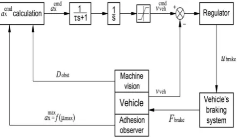
Fig. 1 shows a schematic for the control loop of the automated braking system designed in accordance with the above principles. The “ calculation” block calculates the deceleration command. In addition, the operational range of deceleration is specified in this block in accordance with operational conditions and prescriptions assigned to the vehicle. The distance to the obstacle is transmitted from the “Machine vision” block, while the “Adhesion observer” block performs estimation of the maximum tire-road adhesion coefficient and calculates the corresponding acceleration limit .

filter depicted by the block with the transfer function of a first order dynamic system. The filter prevents the deceleration command from sharp changes, which can be caused by noises in the machine vision signal or by large deviations between the commanded value of the velocity and the actual one. The filtered deceleration command enters into the integrator followed by the saturation block, which output constitutes the velocity command . The actual velocity feedback comes from the vehicle CAN bus (or from other source providing the velocity signal). The difference between the commanded velocity and the actual one is calculated by the sum block and then transmitted into the velocity regulator, which calculates the braking command . In turn, this command enters into the controller of the braking system, which builds the hydraulic pressure exerting the corresponding braking force .

Fig. 1. Control loop of the automated braking system

III. MODEL ANALYSIS OF THE VEHICLE WITH THE AUTOMATED BRAKING SYSTEM For the initial elaboration of the braking control system, operating conditions of the vehicle were considered providing high tire-road adhesion (i.e. maximum adhesion coefficient 0.8 and above). The maximum decelerations allowed by such high adhesion lie beyond the vehicle’s operational range, which mid value is 3 m/s2 and the width is 2 m/s2. These conditions allowed for using a relatively simple mathematical model as a framework for elaboration of the control system for the automated braking function. Low admissible accelerations and high tire-road adhesion made it possible to neglect the latter and consequently do not consider the tire slip. Other omitted factors were torsional stiffness of the mechanical transmission and variable radii of the wheels. Initially, the vehicle motion was considered linear. These assumptions allow one to model vehicle dynamics as a linear motion of one lumped mass, which is driven by the wheel traction/braking force and affected by the resistance forces. The model can be represented as the following differential equation:

where is the vehicle mass; is the torque at the driving wheels; is the static wheel radius; is the wheel rotational inertia; n is the number of vehicle’s wheels; , are the air drag and rolling resistance forces. The grade resistance was neglected since the considered test track was level.

The air drag force is calculated by means of the empirical formula:

,

where is the vehicle air drag coefficient; is the frontal area of the vehicle, is the air density.

The expression for the rolling resistance force reads as follows: , where is the gravity constant, and is the tire rolling resistance coefficient. The latter is approximated by the known empirical formula [13]:

, where characterizes the rolling

resistance at near zero velocity, and is the factor of velocity-dependent growth of the rolling resistance. All the vehicle tires are assumed to have an equal rolling resistance.

Table I contains numerical values of the parameters for the model of vehicle dynamics. These values correspond to the vehicle employed for prototyping of the automated driving system (see details below).

Table-I: Parameters for the model of vehicle dynamics

, kg , m , kg·m2 , m2

1400 0.3 1.2 0.36 1.95 0.009 4·10-6

The vehicle model also includes a simplified representation of the braking system dynamics, which is intended to estimate the influence thereof on the control system’s performance. This representation constitutes a first order dynamic system:

where is the force exerted by the brake mechanisms; is the control signal of the braking system (confined within the range 0…1); is the maximum deceleration allowed by the design of the braking system; is the time constant of the braking system.

The initial elaboration of an automated braking system does not require a transmission model; however, the project implies the full driving automation to be developed, which requires using both the brakes and the accelerator. In order to reflect this within the model, a relatively simple transmission representation was added to it. The vehicle intended for the system’s prototyping (see the details below) is equipped with an automated stepped gearbox. This type of transmission has three operating regimes defined by the state of the clutch – whether it is engaged, slipping or open. In the first two regimes, the engine shaft has its own degree of freedom, which yields the following equation system:

When the clutch fully engages the separate equation of the engine shaft dynamics can be excluded from the model (i.e. lumped into the equation of vehicle dynamics) along with the clutch torque. One can notice that the above equation system does not contain the transmission efficiency. Being taken into account in the actual model, this parameter is omitted here due to its insignificance for the questions at hand.

The described model of vehicle dynamics (containing the model of the automated braking system) was implemented within a simulation software. A number of simulations were performed accompanied by adjustments of the braking control system parameters in order to arrive at the combination thereof providing an appropriate performance of the system. Each modelled experiment included an initial acceleration phase attaining a specified steady speed. During this phase, the vehicle was approaching an obstacle, which

was either stationary or moving at a constant speed. The automated braking system had to intervene and decelerate the vehicle until complete stop (or until attaining the speed of the obstacle) providing a specified safe space between the latter and the obstacle.

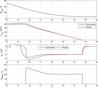
Fig. 2 shows the results of a simulation, in which operating conditions of the vehicle replicated those used in the field tests performed later on. The steady speed to be attained was set at 40 km/h. This value is considerably higher than those prescribed for the developed vehicle by its technical specification. However, due to using of a passenger car (for prototyping purposes), which is lighter and designed for higher speeds than the developed vehicle, it was decided to extend the speed range covered by simulations and field tests in order to guarantee some performance reserve of the control system.

Fig. 2. Results of the automated braking simulation From Fig. 2, one can see that the initial deceleration response

lag caused by actuation dynamics of the braking system is compensated by the increased deceleration command, which takes place in the beginning of the process. The actual deceleration shows some overshoot exceeding the commanded value for approximately two seconds. This appears due to increasing deviation of the actual velocity from the commanded one, which is compensated not only by the deceleration command but also by the velocity regulator, which raises the braking command signal in response to said deviation. When the actual velocity reaches the commanded value, the deceleration command starts to decrease and eventually attains the minimum value of 2 m/s2. When the

vehicle stops, the distance to the obstacle constitutes ca. 5.5 m, while the minimum admissible value was 5 m.

IV. THE EXPERIMENTAL AND THE PROTOTYPING VEHICLES

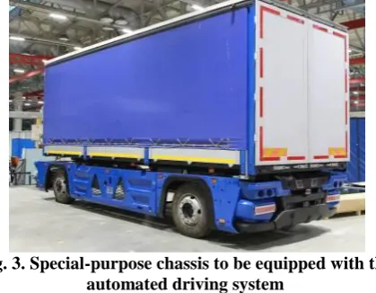
Another modification is removing of the cab as it can be seen in Fig. 3. Since such an extensive transforming is a time consuming process, while the automated driving system should be operational by the time the chassis is ready, it was obvious decision to use a substitute vehicle for the system prototyping. Provided by the project’s customer, this vehicle is a passenger car (Fig. 4) equipped with an automatic transmission. Although this vehicle’s parameters are far from those of the special-purpose chassis, it nevertheless was considered suitable for the system prototyping purposes.

The vehicle that is being developed in the project is based on a heavily modified chassis of a production cargo vehicle [14] (see Fig. 3). In particular, the modifications include replacement of a baseline conventional powertrain by an electric one consisting of a traction battery, a traction electric drive, and a number of accompanying systems [15], [16]. Another modification is removing of the cab as it can be seen in Fig. 3. Since such an extensive transforming is a time consuming process, while the automated driving system should be operational by the time the chassis is ready, it was obvious decision to use a substitute vehicle for the system prototyping. Provided by the project’s customer, this vehicle is a passenger car (Fig. 4) equipped with an automatic transmission. Although this vehicle’s parameters are far from those of the special-purpose chassis, it nevertheless was considered suitable for the system prototyping purposes.

Fig. 3. Special-purpose chassis to be equipped with the automated driving system

Fig. 4. The vehicle used for prototyping of the automated driving system

The automated braking system was implemented within the prototyping vehicle. This included installation of a hydraulic module with electronic solenoid controls into the baseline hydraulic braking circuit. The module provides an automatic regulation of the pressure within the circuit by an external command signal. At the prototyping stage, the braking control system was implemented in the form of a model running in real time on a laptop and being connected to the controller hardware through a USB-CAN interfacing device. The model interacts with two CAN buses, namely, the vehicle’s bus, and the braking system’s bus.

V. EXPERIMENTAL STUDY OF THE AUTOMATED

BRAKING SYSTEM

At the initial experimental stage, instead of physical obstacles (i.e. dummies) a virtual “obstacle” was employed in order to avoid possible unnecessary damage of the testing equipment. The distance to this “obstacle” was calculated from the velocity signal obtained from the vehicle CAN bus (this also did not require using an actual machine vision devices). The field tests were conducted at a horizontal track covered with asphalt. Preliminary testing showed that the maximum adhesion coefficient of this track was in the range 0.9…0.95, which allowed using the version of the control system that did not take into account the tire-road adhesion.

The tests were performed according to the following scenario. The vehicle travels at a specified steady speed when a machine vision system (virtual in this case) suddenly detects a stationary obstacle within a distance requiring an immediate response. The objective of the automated braking system is to decelerate and eventually stop the vehicle at a predefined safe distance before the “obstacle”. The deceleration should be performed within the admissible operational range.

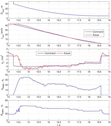
Fig. 5. Results of a road test of the vehicle with the automated braking system

The graphs show that the braking system became active immediately after the detection of the “obstacle”. The time lag of the measured acceleration was ca. 0.2 s. This lag is built up by several factors including raising of the pressure (that began approximately in 7 ms after the braking request), engaging of the brake mechanisms, deceleration response, measuring of the deceleration and feeding its signal back into the control system. One can notice that the dynamics and magnitudes of the shown variables are consistent with those obtained in the simulation. The braking command increases up to 35% and falls towards 20…10% when the difference between the commanded velocity and the actual one becomes smaller. The larger velocity difference in the beginning of the braking is eliminated by a short-time overshoot seen between 14.7 and 15.7 s. After that, the actual deceleration becomes close to the commanded one, and the latter drops to the minimum permitted level of 2 m/s2. The vehicle stops at the distance of 4.967 m from the “obstacle”, which violates the prescribed value only by 3.3 cm. Such accuracy can be considered sufficient. However, one should take into account that an actual machine vision device has limited accuracy and will inevitably introduce distance errors into the feedback signal, which in turn will impair the accuracy of keeping a safe distance. Nevertheless, it is obvious that high accuracy of a system using an “idealized” feedback is a substantial

factor for obtaining a required performance when an actual feedback is introduced.

A number of experiments were conducted in accordance with the described test scenario with various velocities (from 15 to 45 km/h) and safe distances (from 3.5 to 5 m). The obtained results were similar to those presented above including the accuracy of keeping the safe distance. This allowed to conclude that initial assessment of the elaborated automated braking system had proven its operability and satisfactory performance.

VI. CONCLUSIONS AND FUTURE WORK

This command then transforms into the vehicle velocity command, which can be tracked by any kind of regulator that is able to control braking pressure.

The approach was elaborated and tested by means of simulations. Then it was implemented within an experimental vehicle and underwent a field-testing. The experimental results have shown that the developed system operates within a predefined deceleration range (2…3 m/s2

) and is able to stop the vehicle at the exact distance (within 0.1…0.2 meter accuracy) before the obstacle.

The sequel of the described work implies interfacing the braking system with a machine vision system and testing of this extended system using physical obstacles. In addition, the system is supposed to be augmented with a tire-adhesion observer, which will allow introducing a deceleration limitation for roads with low adhesion. When comprehensively elaborated the system will be transferred to the special-purpose cargo chassis.

ACKNOWLEDGMENTS

The article was prepared under the agreement #14.624.21.0049 with the Ministry of Education and Science of the Russian Federation (unique project identifier RFMEFI62417X0049).

REFERENCES

1. H. Winner, S. Hakuli, F. Lotz and C. Singer, Eds., Handbook of Driver Assistance Systems. Basic Information, Components and Systems for Active Safety and Comfort. Cham, Switzerland: Springer International Publishing, 2016, pp. 1177-1206.

2. V. Milanes, J. Villagra, J. Godoy and C. Gonzalez, “Comparing Fuzzy and Intelligent PI Controllers in Stop-and-Go Manoeuvres”. IEEE Transactions on Control Systems Technology, vol. 20(3), 2012, pp. 770-778, doi: 10.1109/TCST.2011.2135859.

3. W. Li, H. Du and W. Li, “Hierarchical based model predictive control for automatic vehicles brake”. Proceedings of the 2017 IEEE International Conference on Mechatronics (ICM), IEEE, February 2017, p. 6, doi:10.1109/icmech.2017.7921152.

4. B. Ganji, A. Z. Kouzani, S. Y. Khoo and M. S. Zahraei, “Adaptive Cruise Control of a HEV Using Sliding Mode Control”. Expert systems with applications, vol. 41(2), 2013, pp. 607-615, doi: 10.1016/j.eswa.2013.07.085.

5. J. Guo, P. Hu and R. Wang, “Nonlinear Coordinated Steering and Braking Control of Vision-Based Autonomous Vehicles in Emergency Obstacle Avoidance”. IEEE Transactions on Intelligent Transportation

Systems, vol. 17(11), 2016, pp. 3230–3240,

doi:10.1109/tits.2016.2544791.

6. P. Senapati, S. Das and P. Vora, “Intelligent Braking and Maneuvering System for an Automobile Application”. Symposium on International Automotive Technology, SAE International, January 2017, doi: 10.4271/2017-26-0080.

7. Y. C. Lin, H. L. Nguyen and C. H. Wang, “Adaptive neuro-fuzzy predictive control for design of adaptive cruise control system”. Proceedings of the 2017 IEEE 14th International Conference on Networking, Sensing and Control (ICNSC), IEEE, May 2017, 6 p., doi:10.1109/icnsc.2017.8000187.

8. L. Wang, Z. Zhan and G. Guo, “Development of BP Neural Network PID Controller and Its Application on Autonomous Emergency Braking System”. IEEE Intelligent Vehicles Symposium (IV), June 2018, pp. 1711-1716, doi: 10.1109/ivs.2018.8500577.

9. J. Yi, L. Alvarez and R. Horowitz, “Adaptive Emergency Braking Control With Underestimation of Friction Coefficient”. IEEE Transactions on Control Systems Technology, vol. 10(3), 2002, pp. 381-392, doi: 10.1109/87.998027.

10. J. Yi, L. Alvarez, R. Horowitz and C.C. de Wit, “Adaptive emergency braking control using a dynamic tire/road friction model”. Proceedings of the 39th IEEE Conference on Decision and Control. Sydney,

Australia, December 2000, pp. 456-461, doi:

10.1109/CDC.2000.912806. 2000.

11. Y. Zhao, X. Xiang, R. Zhang, L. Guo and Z. Wang, “Longitudinal Control Strategy of Collision Avoidance Warning System for Intelligent

Vehicle Considering Drivers and Environmental Factors”. IEEE Intelligent Vehicles Symposium (IV), June 2018, pp. 31-36, doi: 10.1109/IVS.2018.8500568.

12. G. Lie, R. Zejian, G. Pingshu and C. Jing. (6 July 2014). Advanced Emergency Braking Controller Design for Pedestrian Protection Oriented Automotive Collision Avoidance System. The Scientific World Journal. Volume 2014, Article ID 218246, 11 pages. Avaliable: http://dx.doi.org/10.1155/2014/218246

13. G. Genta, Motor vehicle dynamics. Modeling and simulation. Singapore: World Scientific Publishing Co. Pte. Ltd., 2006, pp. 43-44. 14. A. M. Saykin, S. E. Buznikov, D. V. Endachev, K. E. Karpukhin and A.

S. Terenchenko, “Development of Russian driverless electric vehicle”. International Journal of Mechanical Engineering and Technology, vol. 8(12), 2017, pp. 955-965.

15. A. A. Shorin, K. E. Karpukhin, A. S. Terenchenko and V. N. Kondrashov, “Traction module of cab-less unmanned cargo vehicles with electric drive”. International Journal of Mechanical Engineering and Technology, vol. 9(11), 2018, pp. 1903-1909.