Peripheral Production of Resonances

Peripheral Production of Resonances

Geoffrey Fox

Citation: AIP Conference Proceedings

8

, 271 (1972); doi: 10.1063/1.2948694

View online: http://dx.doi.org/10.1063/1.2948694

View Table of Contents:

http://scitation.aip.org/content/aip/proceeding/aipcp/8?ver=pdfcov

Published by the AIP Publishing

Articles you may be interested in

Vector meson production in ultra-peripheral collisions at the LHC

AIP Conf. Proc.

1654

, 090002 (2015); 10.1063/1.4916009

J/ψ production in peripheral collisions of heavy ions

AIP Conf. Proc.

619

, 529 (2002); 10.1063/1.1482484

Glueball candidates production in peripheral Heavy Ion Collisions at ALICE

AIP Conf. Proc.

619

, 525 (2002); 10.1063/1.1482483

Role of peripheral vacuum regions in the control of the electron cyclotron

resonance plasma uniformity

Appl. Phys. Lett.

74

, 1972 (1999); 10.1063/1.123717

Performance testing of a dedicated magnetic resonance peripheral blood flow

scanner

PERIPHERAL PRODUCTION OF RESONANCES Geoffrey Fox*

California Institute of Technology, Pasadena, California 91109 ABSTRACT

We review the peripheral cross-sections of resonances that cannot be produced by T-exchange. Explicitly we consider the four nonets of mesons

n the L = i quark classification, JP = 0 +

~N(980); i +, e.g., AI, B; 2 + , e.g., A 2. We detail the constraints of SU3, exchange degeneracy, fac- torization, pole extrapolation, Watson's theorem and duality as they have been gleaned from long and painful study of well-loved reactions. The controversial nature of the 0 + and I + nonets is related to a surprising suppression of their cross-sections (which are around I0 pb at 5 GeV/c) in non-diffractlve processes. This is explained by a generalized vector meson photon analogy model recently proposed by Kislinger. We predict all differential cross-sectlons for these L = 1 quark states and show that these mesons are best studied in hypercharge exchange reactions, e.g., ~-p + Q0A and K-n § A~A.

An explanation, using final state interac- tion theory, of the large background under the Q and A 1 observed in diffractive processes, sug- gests that quantum numbers of mesons are best studied in non-diffractlve reactions of the type mentioned above.

ON FANTASIES

ON DINOSAURS

ON PARTICLES THAT PIONS LOVE

According to the prophet, research is liken unto a hard and lonely Journey through a torrid, unfriendly desert. From time to time, the barren trek is filled with ecstacy as a lush oasis appears; there our hero may lay down his administrative load and find hidden a piece of the cosmic Jigsaw. After many years, with many toils and just the occasional ecstacy, our hero has pieced together a tiny bit of the cosmos. So with his precious knowledge, he finally returns *Supported inadequately by the U. S, Atomic Energy Commission.

i to the land of the living he left so long ago ...

In this paper, I would llke to record such a trip, namely, a voyage through run-down oases - the homes of disreputable particles

and inconsistent cross-sectlons. Places where even the tarnished

gold of current theories shines like a waxing star.

The next section should have been a pedantic classlflcatlon of various two-body reactions which would delineate the scope of this talk. However, it turned out so boring that I have put it in the first and only appendix. Here I Just note that we will discuss reac- tions of the form:

V?"'

where for the r e s o ~ n c e s M w e will t h e the four nonets of L = I quark states as the lowest-lylng e x ~ p l e s of controversial reso-

2

nances that caunot be produced by T-exchange. ~ e s e are recorded in T ~ l e I. ~ i s t ~ l e should be t h e n with the f o l l ~ i n g grains of salt:

(i) States that can be produced by T-exchange and so are ( c o w paratlvely) s t r a i g h t f o ~ a r d to study are shaded (see Section E of ~ p e n d l x ) .

3 (ll) We tentatively identify the C meson seen in pp collisions as the strange partner of the A I. ~ w e discuss in Section 3.5 under the ~-p § Q0A reaction, this is not a watertight a s s l g ~ e n t . For in- stance, it m y be in the B nonet and further the two Q's - denoted hereafter QA 1 and QB - m ~ mix 4

Table I: L = i Quark States

I - - I

Strange I = 8 9

I = 0 singlet/octet

mixing (?)

0 + Nonet

ZN(980)

K (~ 1250)

c ( ~ 7 5 0 )

s (~ io00)

i + "B" Nonet

B(1235)

QB(1300 § 1400)

h (?)

h' (?)

1 + "AI" Nonet

AI(1070)

QAI = C(?) (1240 + 1290)

D (1285)

D' = E(1422) ? or M(953) ?

2 + Nonet

A2(1310)

(1420)

f0(1260)

f'(1514)

Theoretically the situation is confused by the different mixing schemes. First, we can have "magic" mixing as exemplified by the and ~; in this case, we write the I = 0 particles M (magic -~) and M (magic -~) with an obvious notation. (M* = D or h.) Alternative-

ly we can have essentially no mixing as exemplified by the ~ and n'; in this case, we write M (octet) and M (singlet).

Duality schemes predict h, h' to have magic mixing and D, D' to

6 7

be unmixed The naive quark model predicts exactly the opposite ; here we can only consider all possibilities.

(iv) In Table II, we list the dominant decay modes of the rele- vant 1 + and 0 + resonances. Further we also give either the observed value or SU 3 prediction for the partial widths. Note that the A I nonet predictions might be thought a little hazy as they are normal- ized to an A I width derived (pres-m~bly incorrectly - see Section 2.2)

1 +

Table II: 0+~ Meson Decays

Particle

~ N

(980)

M a s s GeV

0 . 9 8

Decay

Width MeV

Source of Width

(a)

. = "

B (1235) 1.235 ~m I00 Expt

QB 1.380 Kp 32

K ~ 80 (b)

K~ 9

i .01 1.25 1.5

i .07

1.24

1.285 h(octet - ?)

h(magic -~ - ?) h'(magic -r

~p ~p KK + K K

~p

~K

~ I T ~ T

K~

KK + K K

KK + K K

rtot A I

QA I - C

D (1285)

40 330 75

i . . .

140 50

= 21 _+ I 0

50 D' (magic -@)

= E (?) D' (singlet)

1.422 any

(b)

(b)

(b)

(c)

(c)

(c)

Sources: (a) SU 3 and e § ~ = 300 MeV (b) SU 3 and B + ~ ffi I00 MeV

(c) SU 3 and A I § 70 = 140 MeV

The next section is shamelessly pedagogical. Indeed, it, too, almost suffered exile to a dusty appendix. In fact, it is an outline of theoretical weapons we can use to study our reactions. Explicitly we detall the constraints of SU3, EXD (exchange-degeneracy), factorl-

much cleaner in non-diffractive than diffractive processes (in agree- ment with experiment).

In the third section, we analyze the experimental data on the production of the 0 +, i + and 2 + states listed in Table I. The small cross-sections observed for these processes is, a priori, very sur- prising but has a natural explanation in a generalized vector meson

I0

photon analogy model recently proposed by Kislinger The suppres- sion of the I + cross-sections (most of them are around i0 ~b at 5 GeV/c and small t) predicted in Kislinger's model explains and unifies (I) the controversial nature of these particles. (Does the A 1 resonance really exist?) We use SU3, EXD and factorization to pre- dict all cross-sections for these nonets and hopefully the curves in Figs. 9-12 will be useful in planning experiments to elucidate the properties of these particles. In particular, we can note that some reactions (e.g., K-p § Q0n) are difficult because of large background from much bigger T-exchange processes. However, there are others, e.g., ~-p + Q0A ii, where there is no such background and one high statistic experiment could at once settle the vexed question of the properties and even existence of the i + states predicted in the quark

2 model

The final section has the customary pious conclusions but also points out that many of the theoretical conclusions are rendered un- necessarily vague by chronic inconsistencies in quoted experimental cross-sections. This confusion stems mainly from different technical assumptions (mass-cut?, t-cut?, background subtraction?, maximum like- lihood fit?...). It would be nice if such data were recorded in a way (e.g., the horriflc (to some) spectre of a bubble chamber DST bank) that now interest in a particular cross-section would allow a unified treatment of the existing data. At present, one may only smile wanly and hope a now experiment will analyze their data for your favorite resonance and/or in your favorite way.

2: WELL-LOVED FOLKLORE

Here we lay out the weapons to be used in fighting the grimy ogre in Section 3. The order of presentation is less than logical. 2.1: Pole-extrapolatlon

276 e.g.,

G. FOX

I 5

9 I

$ $ I

m

Thus the value is known at t m m 2 in terms of ~-~ scattering and it is only a short (Chew-Low) extrapolation to the physical region (t ! 0). To get the details right requires sophistication (e.g., the poor man's absorption model 12) but rough estimates of the size of the cross-section present no difficulty.

For yector and tensor exchange, e.g.,

. . . ~ "

. , ' ~

>

m m 9

e B $ ~

the situation is similar to the extent that the cross-section at the pole is again an absolutely normalizable elastic scattering (in this

- + T - p +

case ~ p § ). However, the extrapolation is now much more dlffl- cult as one must pass from t = m 2--- 0.5 (GeV/c) 2 to t = 0. It is be-

P

lleved that such an extrapolation is reasonable in the comparable

,....) ....

~o

"I . . . . ~ ~ '

ratio of amplitudes for ~-p § A~n over ~-p § TOn; this cancels the un- known p § NN coupling. Thereby we relate:

d ~ / d t ~ - p + A ~ n ] r(A I § ~ )

to (1)

do/dtE~- p § ~On] r(p § ~ ) We can make two remarks on (I).

a) Clearly the same method will work for all I + production by vector exchange. Again, for tensor exchange reactions (e.g.,

w-p ~ B0n is pure A 2 exchange), we need not extrapolate all the way to the A 2 pole but rather use SU 3 and EXD (Section 2.4) to relate (in this example) A 2 § ~B to ~ § ~B. So, in the general i + reaction, we need only extrapolate to a vector meson pole in order to estimate the cross-sectlon.

b) In Section 3, we show that (I) gravely overestimates the cross-sectlons for production of the A I and B nonets. So we need not worry about niceties in (I). For example, different choices of in- variant/heliclty amplitudes in (I), can give a factor of 2 difference in the extrapolation prediction. However, this is an irrelevancy when faced by an order of magnitude discrepancy with experiment.

2.2: Watson's Theorem

a) "Theory" - This states that in any process, e.g.,

the amplitude for production of an eigenchannel 34 is proportional to 16

e where 6 is the phase shift for the same eigenchannel in

$

- . . ) W "

. )

(2)

for m ~ m and projecting out spin J = I, we have only one elgen- channel - the I = I, J = i ~ channel which is then proportional to

if

e - the phase of the corresponding

~ ' . . ) . . . .

~ . W "

vv~'

9 .

,~..Q'.'.

,).'

.'~*

(3)

amplitude. This is, of course, Just the usual p Breit-Wigner phase. if In (3), the (elgen) amplltude's phase is completely specified by e . It is important to realize t h a t this is not the case in (2) where one has additional sources of phases, e.g., Regge theory would give phases:

(exp

for the ~,A 2 exchange contributions. One can still use the theorem if you realize t h a t - lapsing into the language of my childhood train- ing - every such imaginary part is associated with the discontinuity across a total (e.g., s in (2)) Qr sub- (e.g., X) energy cut. Then the Regge phase (4) is associated with the w-p and ~+n thresholds in

- +

(2) and has nothing to do with the ~ ~ threshold. Granting this, 13

one can s t a t e Watson's theorem as :

Any sub-process in any scattering process is associated with a branch-cut in the corresponding s u b - e n e r ~ in t h e ana-

lytic function that is the scattering amplitude. This branch- cut generates an imaginary part whose phase is $iven by

Watson's theorem.

14 impossible but we can state the following rule

Watson's theorem never predicts absolute phases. However~ if a final sub-process has a rapidly varying - as a function of the sub-

if

energy X - ei~enphase e ~ then the production amplitude will exhibit essentially the same phase variation in this ei~enchannel. The condi- tions of this rule are presumably satisfied for a resonant eigenphase.

It is perhaps instructive to go through this in detail for a 2-particle sub-process. Then the discontinuity version of Watson's

13 theorem is symbolically :

. . ( 5 )

where the @ signs denote one's position relative to the s34 old cut in the scattering amplitudes,,

i.e.

thresh-

§

ffi

Such amplitudes have a square root branch point at s34 = Sth. So we write

ffi T = A + iw

where B = B~s34 - Sth

(6)

iS

amplitude as e Sin ~ gives

I/2i E(A + iB) - (A - iB)] ffi (A + iB)e i~ Sin

or putting C - B/Sin

(A + i B ) = e i 6 C. ( 7 )

H e r e C h a s n__oo s34 s i n g u l a r i t y a t s34 - S t h b u t i t d o e s - l i k e A a n d

- h a v e t h r e s h o l d s a n d , h e n c e , i m a g i n a r y p a r t s c o r r e s p o n d i n g t o a l l t h e

o t h e r s u b - e n e r g i e s . (7) i s t h e n t h e m a t h e m a t i c a l f o r m u l a t i o n o f t h e r u l e we s t a t e d a b o v e .

b ) A p p l i c a t i o n t o o u r r e a c t i o n s

Watson's theorem is powerful if (and only if) there are but a few open channels, and so but a few elgenstates. This is the case for all the resonances w e are considering here. For instance, in

. . .

i ~ B

i + ( ~ s - w a v e )

at s ~ , we deduce that the JP ffi is ~ e ffi i at res-

onance where ~B is usual Breit-Wigner phase shift for the B. Mean-

+ P = - _ =

while, the -JP ffi I ( ~ D - w a v e ) , J 0 ,2 states are exp ( ~ O i ) as these states are (presumed) non-resonant. Note that the 'background" in a given elgenchannel must have the resonant phase; it need not have the resonance pole.

c) Fantasy

I would llke to use the above formalism to divide hlgh-energy peripheral scattering processes into two basic types:

9 Sin ~ Production

(i) Direct channel formation - including photoproductiou.

(ii) q-exchange processes at smell t.

(lii) (?) Other non-diffractive processes at high energy and smell t.

e Production

(iv) Diffractive processes.

(vi) (?) Electroproductlon - High q2. (vii) (?) All reactions at high -t.

To understand the distinction, consider some examples. (i) Direct Channel

We can w r i t e (5) as

, *

T - T = 2iTT 2

where T is the multiparticle and T2, the T -~ 2 amplitude. thus a linear (in T) unitarity rel~tion. 2At low energies

9 9 . . W § I ~ * .

(8)

It is , say,

we may put T = T 2 whence unitarity becomes a non-linear constraint which implies

T 2 ~e i~ Sin 6 (9)

where the "extra" Sin ~ factor comes from the non-linearlty of the unitary equation.

The amplitude (9) peaks at resonance (6 = 90 ~ ) and vanishes w h e n = O. Correspondingly, a Breit-Wigner parameterization is valid and resonances are produced very cleanly at low incident energy for there are only a few competing eigenchannels.

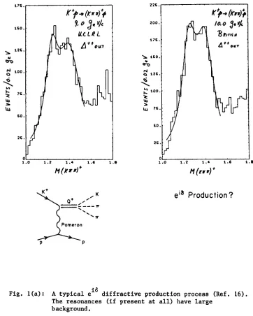
(iv) ei~: Diffraction Production

e.g.,

Now

el8 i8

T ~ Sin 8 but only that T u e . We deduce that there w i l l be no large peak at resonance (8 = 90 ~ ) 15 and also that the cross-section can be non-zero even if ~ = 0 (or 180~149 It follows that it is in- valid to use a Brelt-Wigner parameterization in such processes. For

instance, the latter implies zero cross-sectlon when 8 = O, a predic- tion w h i c h is manifestly wrong. In any case, dinosaurs apart, we deduce resonances w i l l b e produced with large background 9

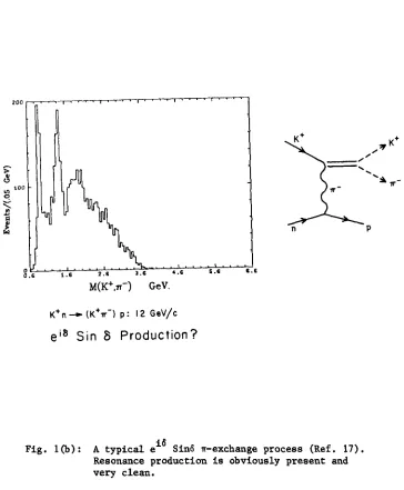
(ii) e i~ Sin 8: ~-exchan~e

9

K §

9 ~, . . I , ( + 0 .

9

I

i i 9

.A~-

'> .""

I

is proportional tc e i8 Sin 8, rigorously at t = m 2 ~, and will remain so

for small t (in the physical region) as pole extrapolation is valid 12

for ~-exchange . Thus resonances produced by n-exchange w i l l be clean and accurately described by a Breit-Wigner.

These points are illustrated in Fig. i which compares the

e 18 K+p § ( K ~ ) + p diffractive reaction 16 with the e i8 Sin 8 ~-exchange process K+n § (K+~-)p 17. Manifestly, the resonances are much cleaner

18 in the second case

(iii) eiSSin 8 (?): Other Non-diffractive Processes

19 The case of the vector and tensor exchange processes , of interest for Section 3, is less clear. If pole extrapolation is even qualitatively right, then Regge exchange is proportional in, say,

. .

e 0 9 0

9 0

2 to beautiful e i8 Sin 8 ~ elastic scattering at t = m . My

g u e s s i s t h a t t h i s w i l l e x t r a p o l a t e 20, and such r e a c t i o n s w i l l

P

1 5 0 .

~LC L I~ L

1 2 5 .

~ I O 0 .

c o .

. /

1 . 0 1 ' . 2

2 2 5 .

2 0 0 .

1 7 c .

1 ~ 0 .

r

<

~ IOD

50.

25.

M(~,,)*

M(-,)"

Io.o 3"~

I . B

Q+ /_C~'E K

P P

e i8 P r o d u c t i o n ?

Fig. 1

(a)

Z O O , ' " , ~ - ~ 9 = , ~ - ' T . . . . u . . . . i . . . .

v ~ 0 0

. G t . G 2 . G 3 . G 4 . G ~ . 1 ~ r

M ( K + m -) G e V

K+n.--~ (K+~ --) p: 12 GeV/c

e is Sin S P r o d u c t i o n ?

K + K +

f

"~,~ _

n P

indeed be e i~ Sin ~ for small t. However, the low cross-sections make it impossible to find any conclusive experimental evidence either way.

We note that the Pomeron processes have no pole to extrapolate 21

to ... so w e cannot find the missing Sin ~ factor. Let us speculate:

(v) e : Medium Energy Non-diffractlve Reactions

At Plab < 5 GeV/c, there will be some contribution, say to A 1 production of the form

l-

;t

(lo)

where the " r e - s c a t t e r i n g " O ( i n I0) will give e i~ not e i~ Sin ~ pro- duction. Theoretically, such a box diagram is a Regge-regge cut and it falls fast with energy (~cut ~ -I in this case). Thus one might deduce that non-diffractive resonance production will become cleaner as energy increases and e i~ Sin ~ Regge Dreamland is approached.

(vi) Photon Processes

Consider photo or electro production, say, vN + wN where the photon has mass q2. At q2 = O, vector dominance (VDM) is roughly right and our amplitude is proportional to pN * ~N which is a nice

i ~ 22

e Sin ~ formation reaction of the type discussed in (i) . How-

2 i6

ever, for larger -q , VDM is inapplicable and so one would expect e production. We deduce that resonances should have increasing back-

2

ground as -q increases.

Similar remarks can be made about inelastic electron scattering which essentially measures ~tot(yp § 7P). At low 7P mass, unitarity may b e used to relate this to sum of single photon processes 9

(vN § ~N, ~ N ) . Again one predicts less background at low q- due t o

the effects of VDM non-llnear unitarity giving "e i~ Sin 8" resonances. 23

This prediction appears consistent with the current data .

in which, liken unto diffraction scattering, resonances sit on large background. Unfortunately, as I have often lamented 12, 24, there is no serious experimental study of this important domain.

2.3: Duality

We will use duality in 2.4 to conclude that, say, K + n § Q0p is real at high energies with EXD p, A 2 exchange. This is very reason- able ...

However, one could also use it to relate:

. . ~ .... . ~ , ~

".~...

~.

~

~

, '

- -

"

9 9

~.

.."

- , -

,.--,S'

1 " '

However, the ~ and ~p sub-energles are clearly too low in these cases for duality to be useful. It is reasonable to use it for relat- ing

9 e l f ee 9

e 9 e e

"r..;.,:"

" ' ~ . . ~ .

~.

~P;~

S"

.. 9

,..,:~

e e

(13)

number of eigenstate situations where duality is at its weakest. The deduction for our discussion in Section 3 is that I believe it makes little sense to consider exchange (p in (Ii), ~ in ( 1 2 ) ) e x p l a n a t i o n s of data at these low sub-energies.

It is perhaps useful to make some remarks on (12) - the Deck model Dinosaur:

(i) I once believed the Deck model was a reasonable description of diffraction because of the ~ pole in

:"

However, this is not correct. Thus, at tVp =^tpomero n = 0, it is easy to see that the residue of the ~-pole(t 0 = m~)_ vanishes. The easiest w a y to prove this is to note that the Deck amplitude is proportional

25 to

( ~ p = I)

I s 2 (14)

2 t -m

where w e mark s, s I and s 2 in (12). But at t~p = 0, we find

2 m - t

s 2 = ₂

(s I - m )

9 s (15)

Combining (14) and (15) we find no w-pole in the resultant amplitude. This has in fact been known for a long time 26 _ it is the "successful" prediction of an s-wave A I. However, it has not been emphasized that it implies zero w-pole residue.

, " :

..

'J.~"

'~"

all give identical forms for the amplitude~ Now, 27

if we replace the Pomlron by a photon - to w h i c h i t is kine- matically identical - then gauge invariance implies all three dia- grams in (161 add up to give identically zero in the forward direction

(i.e., for real photons of zero mass). In this case, it would be di- sastrous to take Just 16(a) and ignore 16Co) and (c) 28.

(iii) W h a t experimental evidence is there for the Deck model? There can be essentially none for its really distinctive predictions - for as we described above it has no distinctive features and all three diagrams in (161 are kinematically identical. There are s o m e predic-

tions of relative cross-section sizes... But a recent SLAC experi- ment 29 has shown that it gives the wrong answer for --KUp § Q0p v. ~0p § ~0p (Fig. 2). We can only conclude that the "success" of the

26 Deck model was based on its correct multiparticle kinematics virtue shared by many diagrams.

So finally, we turn our fancy towards more humdrum things. 2.4: SU3, EXD~ Factorlzation

-- a

(i) Denote the well-loved particles as follows: P : Pseudoscalar honer 7, ... ~'

V : Vector honer p ... N : 89 octet p ... A

D : 3/2 + decuplet A(1234) ... O- Denote the well-loved Regge exchanges: V : Vector nonet p ...

T : Tensor nonet A 2 ... f' B : B nonet B ... h'

N

>

0.01

' I ' I ' I

DIFFERENTIAL CROSS SECTION

4 <PBEAM<I2 GeV/c

o ~Op__..~Op

9 K~

Q~ p

0

0.2

0.4

0.6

-(t-train) GeV 2

Fig. 2: Crossover at t ~ - 0.2 (GeV/c) 2 between KOp § QOp and ~Op § ~0p (Ref. 29). The scale, unlike Fig. 5, is nor-

+

Normalizing one coupling

i v

in w h a t e v e r w a y w e please, one can use factorization and EXD to find all six Regge vertices.

p

P

Each of the six couplings - on using S U ^ - leads to the couplings of individual members of the multiplets. J(This needs the known D/F ratio for

(iii) Further, da/dt and density matrix element data on say ~-p § wOn, K-p § A~ 0 allow one to separate the unnatural parity coup- lings from the natural parity vertices discussed above, and so obtain

all the amplitudes ,

+ +

Then SU 3 and EXD will give all such couplings

for meson resonances in a given multiplet. Coupling this with the general N~, ND vertex, we deduce: Given da/dt for one meson resonance in a multiplet~ we can at once predict all cross-sectlons of the form

* 9

P N + M N~ P N § M D.

As always some caveats are necessary:

(v) If the M*'s form an unmixed nonet (as do the ~...n'), then it is illegal to use the quark model rules (i.e., no disconnected quark diagrams) to calculate the singlet cross-sectlons. This sin overestimates the singlet cross-sectlon by a factor of 4 in the case of the ~...n' nonet 31. In our application, we don't really know what any mixing angles are; so we shall forget this difficulty and, for definiteness, use the simple quark rules.

(vi) One can estimate, say, the coupling . ~ . . ~ ~

using EXD and the known

. T

/.

coupling. This is the tensor analogue of the ~-B exchange degeneracy 32

argument to relate p and ~ production . EXD is not perfect in the latter case, and one might assume a similar breaking for the tensor production. Then, symbolically, we have:

i m m i

tO ).

(vii) Absorption will modify some of the above results. All our results involve taking ratios and so some absorption effects cancel. However, the ratios involve different spin amplitudes with "Born-

terms" of different t-dependencies. So, as the absorption depends on these effects, it certainly should not cancel completely. However,

24

nobody can calculate the desired corrections and so we shall com- pletely ignore them hereafter.

3: PRODUCTION OF THE L = 1 Q U A R K M O D E L STATES 3.1: Strategy

According to the discussion 2.4, one need only isolate the cross- section for the production of one member of any nonet to be able to use SU 3 to predict all others. Our knowledge of well-loved reactions enables us to guess the most favorable processes. Thus,

and

have large NN spln non-fllp amplitudes. Thus, they correspond to large cross-sections. ~

^

s

is also mainly non-fllp but its size is suppressed; however, this is the usual strange particle production suppression. So K ' exchange may be expected to produce resonances with a smaller cross-sectlon

than ~ or fO exchange but with a similar t-dependence and a comparable signal/ background. On the other hand,

P

and

are

dominantly spln-fllp and give rather measly small and flat cross- sections.

data is less certain simply because of the low statistics implied by the universally small cross-sectlons for associated production.

Let us look at some specific examples. However, first~ a moment of sadness. Throughout this section, there will be no such thing as a clean prediction - unsullied by theoretical or experimental caveats. Rather, time after time, we must swat at monstrous factors of two as, devil-horned and dirty, they cling and infest the cross-sectlons of our desire. We Just state the difficulties and record our compromises. 3.2: 2 + Production

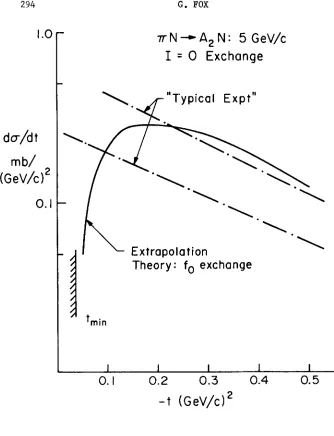
Consider the processes ~• § A~p around 5 GeV/c.

(i) There is a large fO exchange contribution 34,35. Any such vector or tensor exchange must be hellclty flip at the ~A 2 vertex; parity forbids the coupllng ~A2(hellclty 0) § V,T. This prediction is confirmed by the density matrix elements observed for A 2 production

33 at higher energy

(il) Helicity zero A2's can be produced by I = i, B exchange - this amplitude is now spin-fllp at the NN vertex and so both f0 and B exchange predict A 2 production to vanish in the forward direction. One can estimate B exchange using EXD (cf., Section 2.4) but rather one eliminates both B and O exchange (cf., Fig. 9, the latter is the smaller of the two) by forming the I = 0 exchange combination.

+ ~-p

do0/dt = 89 do/dr - {~+p § A2P + § A2P - 2(~+n § A2P)} . 0

(1~)

34

( i i i ) E q u a t i o n (17) has b e e n d i s c u s s e d by Rosner , b u t u n f o r -

t u n a t e l y currently quoted experimental cross-sections are simply in-

consistent 34,36 So in Fig. 3, we mark a range of experimental dif- ferential cross-sections. This is compared with the absolute theoret- ical prediction given by the pole extrapolation model (i.e., the ob- served r(A2) § nO plus SU 3 and EXD gives coupling ~A 2 § Regge f0 at

2 t = m0).

The qualitative agreement between theory and experiment in Fig. 3 appears to me rather impressive. The pole extrapolation gives both roughly the right absolute magnitude and a reasonable (e ~3t)- t depen- dence. It's interesting to note that this reaction is dominated - theoretically and experimentally - by a single spin-fllp amplitude. Such an amplitude is known 24 from study of well-loved ~-p + (~,n)n, etc., to be the (only?) case where simple Regge theory gives good pre- dictions. So it was probably to be expected that pole extrapolation

(which implicitly assumes perfect Regge theory) would work. 3.3: B Production

1.0

d /dt

mb/

(GeV/c) z

0.1

TrN--~A2N" 5 GeV/c

I = 0 Exchange

~ .

~

~

a

l

Expt"

A

Theory: fo exchange

train

I

I

I

I

I

O. I

0 . 2

0 . 3

0 . 4

0 . 5

-t (G eV/c) z

again vary within a factor of 2 (~) but qualitatively the size and shape of ~+p + B+p is similar to ~N + A2N (I = 0 ex-

4O

change) . Theoretically the situation is quite different; again, we have a large (as defined in 3.1) amplitude: this time ~ exchange. However, parity no longer forbids the wB (helicity 0) ~ coupling and we expect a dominantly spin non-flip amplitude rather than the spin- flip which controlled A 2 exchange. This should give a large and steep (i.e., exp(~ 8t~ d~/dt. Indeed, given F(B § p~) ~ F(A 2 § ~0~ pole extrapolation implies qualitatively

de/dt (~N § BN) ~ m~/t de/dr (~N + A2N) (18) This is made quantitative in Fig. 4 which compares the precise pole extrapolation prediction with experiment. As anticipated above, the theory is a complete disaster - being a factor of 30 too big in the forward direction. Figure 4 marks the ~B spin-flip (i.e., B heli- city • I) part of the theoretical cross-section. It agrees much better in both shape and size with the data. Combining this with the

similarity of the A 2 and B cross-sections, we conclude that the latter is largely spin-flip. It follows that it is a matter of theoretical urgency to understand what has happened to the B helicity zero ampli- tude.

3.4: Kislin~er's Model

In Kislinger's model I0, the vector meson Regge pole couplings are proportional to those of the photon. In the case of

\ .

V ~'~

(e.g.,

§ NE),

this is well known to give the successful prediction of the

I 0 -

1.0

do-/dt

m b / 2

(GeV/c)

O l

C. FOX

" ~ E x p t :

5 GeV/c

t I

train

8

Expt" 8 GeV/c

Tr + p --- B + p: 5 G eV/c

"-~.+ a . -''IT+

.... CO 0

P

FullPTheory

".. ~

... ~-exchonge, oll

"... ~

spin stores

9

~

- - - -

u~ + A z exchonge,

".... ~

spin-flip only

/ ~ ~

",,

t ) -

"

9 ~

I

I

I

I

I

o.I

0.2

0.3

0.4

0.5

- t (GeV/c) 2

F• 4: Comparison of w+p § B+p data (Refs. 37 & 38) scaled t o

9

where a and b have spin 0-. This can be written

T~ = X(qa - qb )~ + Y(qa + qb )B (19)

for invariant amplitudes X and Y. Gauge invariance, i.e.,

qy~ Tg = 0 : q7 = qa - qb

(20)

implies

Y(m - * Xt = 0 ( 2 1 )

i.e., for inelastic scattering, m a ~ mb, Y vanishes at t = 0 (t = q~). X plays no role in the scattering at high energy (e.g., it is and so its contribution vanishes when dotted into the lower ver-

qy _,

tex 7 § NN, NB ). Thus the non-flip y § ab amplitude is proportional to Y and hence t as claimed.

Finally we note that Kislinger's model has all the SU3/EXD fac- torization properties discussed in 2.4. So no considerations based on this are affected. Also we should note that the SU 3 formulation means that we avoid the embarassing prediction that ~N § KA vanishes at t = 0. (Putting a = ~, b = K in (21) would naively give this disaster.)

3.5: Production of the A 1 N o n e t

This is a particularly tricky discussion because there appears to be a discrepancy between the diffractive and non-diffractive data. There are two important new sources of information on 1 + diffraction. First, the Illinois partial wave analysis 42 of the 3~ system in ~-p + (~-~-~+)p; second, the SLAC data 29 on KOp + Q0p. I discuss these in turn.

(i) A I Diffraction Production

42 A very surprising feature of the 3~ partial wave analysis in

~-p +

( " A I " , A 2 "A3" § 3~)p

2.2 that Watson's theorem implied that there could well be little connection between resonance positions and bumps in the mass spectrum. However, one "had to" observe relative phase-variations. In this case, one should see the phase of the resonant I + (S-wave) A I compared to the 0 background. One could advance five explanations for the lack of observation of this effect.

a) The A I does not exist - I reject this because of the impres- sive evidence for its SU 3 partner: the D meson.

b) The 0- has a similar resonant phase variation to the A I. I ~ J e c t this "daughter" possibility as being implausible at~such a low mass.

c) The A 1 is not a "narrow" resonance at 1.07 GeV. Rather, it is a broad effect centered at (presumably) higher mass. For in- stance, if its mass was 1.285 GeV, one would expect a width of 230 MeV. This possibility has to be taken seriously because experimentally - the mass of 1.07 GeV comes from a probably un- justified (in "e i~ processes" - see 2.2) association of reso- nance position with a bump in the same diffraction data that sees no phase variation. Theoretically the mass formulae based on the quark model are, I believe, completely empirical and could be adjusted for a new A 1 mass. There is the notorious pre- diction mAl ~ m p which agreed miraculously with 1.07 GeV; however, this should not be taken seriously.

d) Final state interaction theory is wrong. For instance, our rule in 2.2 stated that only "rapid" phase variations should be detected. What total width corresponds to "rapid" variation? An important check of these phases would be the experiment 44

P

P

using the Argonne polarized proton beam and detecting the fast

+ 0

n, ~ p system. This experiment has three advantages over the ~p reaction:

~) The two particle ~p state is easier to handle than the 3~ "AI" decay - cf., my objection (e}.

8) Polarization is more sensitive to phases than cross-section. y) The wp resonances, i.e., phases, are better known than

their 3~ counterparts.

e) The data analysis is unreliable for a delicate interference question llke the A I phase. Against this possibility, we have the analysls's successful isolation of the A^ phase 43. On the

z

In conclusion, the 3~ partial wave analysis - of which we have three reasonable interpretations, (c) to (e) above - casts serious doubts on the usual A. parameters. However, it doesn't directly tell

I

us anything about non-diffractive production. (ii) q0 Cross-over

Let P be the diffractive and R the non-diffractive contribu- tion to

K0p + Q0p. Then, according to f o l k l o r e 45,

daldt,(K0p § Q0p) = [p12

2

(22)

do/dt,C~0p § ~0p) = ip + R[

2 29

A SLAC group has used these equations to isolate R as ImR = do/dt'

(QOp)

(23)

Their data is shown in Fig. 2 and the value they extract from it for IRI 2, i.e., the non-diffractive contribution to Kp + Qp, is shown in Fig. 5. The latter requires a lot of explanation.

The experimental data corresponds to a simple mass-cut

i.i ~ M ( K ~ ) ~ 1/5 GeV and has been corrected for unseen decay modes. For this definition of the Q, the value one obtains for IRI 2 is too large to agree with two other methods of calculating it. First, we

I0

have Kislinger's model which predicts that Q like B non-diffrac- tive production should vanish at t = 0. So any non-flip amplitude

(which is that measured by (23)) must be small. Second, we have the ~-p § Q0A data ii to be discussed soon. This shows, in perfect agree- ment with Kislinger's model, a small flat d~/dt which is, in turn, inconsistent with a large non-flip amplitude. So we assume that most of the "mass-cut Q" observed in the K U experiment corresponds to

(e i~) background. Perusal of the mass-dependence of the similar K+p § Q+p data 16,47, suggests that with the QAI parameters of Table II one could assign about 88 of the SLAC cross-section to the true resonance QA " This has been done in Fig. 5.

I

Given the above, this figure now exhlbits the usual diasgreement between experimental cross-sections and pole extrapolation. Without the mysterious factor of 88 we would have agreed with pole extrapola- tion but not as discussed above with either Kislinger's model or ~-p + QffA.

Note that Fig. 5 suggests sizeable non-diffractive Q production 46

300

I0

I.O

d~/dt

m b / 2

(GeV/c)

0.1

G. FOX

Kp--OA, P (~,

fo Pomeron exchonge~

, Extrapolation Theory-full

}Nondiffractive

- - -

Extrapolation Theory-spin-flip

Theory

- - -

I / 4 (K ~ p_,..QO p: 1.1< m(K*rr)< 1.5)

\

,~ ~,,mo,e O,o;O?,,o, OC,,ve oor,

/ 1 - - ' - . \ \

- [

~ \ \ "

ooto

I

I

I

I

I

o l 0.2 0.3 0.4 0.5

-1' (G eV/c) 2

(iii) ~-p + q0A

We now come to the most convincing evidence for non-diffractive production of the QA 1 or QB" This comes from a study Ii of

~-p + ( K ~ ) 0 A at 4.5 and 6 GeV/c. The K ~ mass distribution, shown in Fig. 6, indicates a sharp peak at M ( K ~ ) = 1.29 and a broader en- hancement around 1.4 GeV. There are three possible interpretations

of this data.

(a) The first peak is identified with the C meson observed in pp annihilations around M ( K ~ ) = 1.24 GeV 3. The mass difference is

attributed to background interference. This first Q is then QA 1 while the enhancement at 1.4 GeV is a mixture of K1420 and a second

relatively narrow QB resonance.

~ ) We have the same identification of the first Q as the C meson but we assume it is QB" Then by analogy with our interpreta-

tion (c) of the Illinois A 1 analysis (3.5(i)), we assume the QA 1 is much broader and hence indistinguishable from background. For in- stance, the mass assignment M(QAI ) = 1.35 GeV doubles the expected width and mixing may do other awful things.

(c) The 1.29 enhancement is QB while QA 1 at lower mass (i.e., 1.24 GeV) has too small a cross-section to be seen.

Examination of the do/dr' data for the two regions (I: 1.24 < M ( K ~ ) ! 1.34, II: 1.34 ! M ( K ~ ) ! 1.48 GeV) rules out (c) but with- out ehough data to allow a partial wave analysis, one cannot distin- guish (b) and (c). The data in Figs. 7 and 8 comes from a DST kindly sent me by Kwan Lai and Howard Gordon with normalization taken from

48

the standard compilation . For theory, we use SU 3 estimates of the type discussed in 2.4: that for ~-p § Q~A uses ~+p + B+p; that for

- + 0

P QA uses the SLAC K0p § Q0p crossover analysis 29 for normali- I

zation and the Kislinger model I0 for t dependence; finally for

- p § * + + *

KI420A we use ~-p + A~p. This underestimates the K1420 cross- section by a factor of 2 because it omits a sizeable K and QB e_~x- change contribution. This can be seen theoretically from the EXD ana- lysis of 2.4 and experimentally 11

by

- * 0

p + KI420Z . (The latter has no ~ exchange.)

Finally we can actually examine Figs. 7 and 8. First, we note the beautiful agreement between the t-dependence of theory and ex- periment. This flat t-behavlor again supports Kislinger's idea that

all such resonance production (Q , Q .j K,~,~) is mainly spin-fllp. B 0 A I ~ L u

302 G. FOX

e i8 Sin 8 Production

6 0 -

BNL

Data

rr-p--~(K~-~) ~ A 4.5,6 GeV/c

Y * o u t

c o s 8 p , A > 0 . 5

K* or p

selection

1.29

1.42 ~ l

~. 7'r

_,,

_{Qo t-.-K}

/

p .n.

co 4O

20

f-

I I I I

1.0

1.2

1.4

1.6

m (K-rr-rr) GeV

1.0

_{r - p " " (K 7rTr) ~}

_{A =}

_{5 GeV/c}

Data is BNL P0ab = 4.5, 6 GeV/c

1.24 < m (K-tr'n') < 1.34 GeV (Y* out)

0.1

SU 3 for w'N--~ QBA

using w "+ p - " B+p data

SU 3 for TrN --'~ QA, A

using K~176

data

d -/dt

m b /

(GeV/c) 2

0.0

. . . .

J g

~tmi n (m : 1.38)

I

I

I

I

I

0.1

0.2

0.3

0.4

0.5

- t , f f (GeV/c) 2

Fig. 7: "Lower Q": Experimental mass-cut data (Ref. II) compared with SU 3 predictions for QAI and QB"

0 . 1 - -

d /d,

m b /

(GeV/c) 2

.01

-

m

"rr-p---~ (KTr-rr) 0

A ~

5

GeV/c

BNL Data: Plab = 4.5, 6 GeV/c

1.34 < m(KTrTr)< 1.48 G e V : Y * o u t

0;ii,i''"

I

I

l

I

i

0.1

0.2

0.5

0.4

0.5

-tell (GeV/c)z

assumptions in our interpretation of the SLAC QA I data. Note that this curve does include the magic factor of 88 discussed in 3.5(ii) and would have been far too large without it. Given the SLAC QA

1 curve is not still miles too big, we can rule out possibility (c~ be- cause there is not enough "spare" cross-section at low K ~ masses. 3.6: Predictions

Using ~+p § B+p and ~-p + Q0A (assuming the 1.29 GeV enhancement in Fig is QAI ), we can now, as described in 2.4, use SU 3 to predict the cross-sectlons for all members of the B and A I nonets. The re- suits are given in Figs. 9 to 12 where we have also marked some typi- cal do/dr for well-loved reactions. The calculations are arbitrarily given for Plab = 15 GeV/c; they can be scaled to your favorite mo- menta using the usual ~lab-2=-2 (= ~ 0.5 non-strange; ~ ~ 0.35 strange- ness exchange) scaling law. The only exceptions to this are first, the two B exchange reactions ~-p + ~N(980)n and ~-p § A~n. These

p -2 and the plotted cross-sections were ~ calculated scale more llke lab

using the ~-B EXD ideas described near the end of 2.4. Similarly for their strange partner 49 K-p § ~N(980)A in Fig. II(II) which is K and QB exchange, I have assumed Pla~ scaling.

As indicated in the introduction, the epithets magic-~ (sometimes abbreviated to magic), magic-~, octet and singlet describe possible mixing schemes of the I = 0 D and h mesons. Further, we do not mark explicitly the ~+p § M*0A ++ cross-sections (which are essentially

M*0n * +

identical to the analogous ~-p § reaction) and K-p § M*-YI385 , *+ *+

~+p § M Y1385 which are rather small (see ratio 50 of ~+p § K+E+v. g+p + K + Y ~ 8 5 in Fig. i0(I)).

3.7: Further Tests

Now we would like to test our predictions in Figs. 9-12 by com- parison with various other reports of i + production in the literature. These are generally not as statistically significant as the reactions in 3.3 and 3.5, but it is important simply to check that our theoret- ical predictions are no larger than current experimental upper limits.

(i) CEX q: K+n ~ KOp, K-p § Q0n

306

1.0-

_{(I) 7T-p--- n: 15 GeV/c}

_M*

-rr- p --,- pO n,

~

~T- p--"

fOn

\

",,

\

M ~

Decoy

---~. -/T + -iT -

o l ~ \

! ~ . " \ ~ q -p'~Tr~

B +- Tr + - 7 r -

-o?n

\

" Tr+-

p---

B• p

---,- w

do-/dr ~

.

,

.

rob/

~

- ~ .

" ~ . .

Tr- p--,-

B~

(GeV/c)

z { " "

~ ~ ' ,

--" ~ ~

o.o, K

~

~ OCmo~,~--- ~,~

D'(singlet) ~ KK~T

/ ~ ' ~

~

O(octe,)---,- KK'rr

/

\

i

\

TT N ( 9 8 0 ) --.,,- "ft"T']

l

{

I \

i

l

o.,

0.2

0.3

0.4

0.5

-t

(GeV/c)2

Fig. 9

(x)

:

I.O

o.I

do-/d t

mb/ 2

(GeV/c)

OO1

Fig. 9 ( I I ) :

(Tr) -rr- p -,,- M * n 15 GeV/c

\

\

\

\

p-,,-

_

"~

-rr-

pO, fo n

\

"----~

-

".\Tr-

p ~ ~TOn

-rr-p--~ ~n

• ~ _ ~ . , , ~ x

e ~ 9 i o o ~ mo J o

o e 9 ~ ~ 9 o

.... . . - _ \

Y,

" . " X 0

_

" ' ~

"..

~2(B exchange)

...

". \

. . . - /

-...->•

..

/

-

~ \

9

-/~o

':'~ '" "

(p exchang

e l L X ~ i l . "''" h (magic)

".... ~(singlet)

h (octet)"

~

AO ' %

/4 I

I

L

I

I

I

o.I

0.2

0.3

0.4

0.5

- t (GeV/c) 2

All M*'s

decoy

into

308

0.1

G. FOX

(I) "rr+p - , " (M *+---~ Kn--rr) 2+: 15 GeV/c

.Ol

do-/dr

m b /

(GeV/c) 2

.001

"rr+p-'~K+ T. + (14 GeV/c)

I ',~

~

~-+p----, Y,&;, (14GeV/cl

... :X,!.. ~

}

9

...{...~... { ~

x ~ x ~ x ~ x ~ x~ ~ ' ~ ' t ' ' "

QB

/

* ~

-

x ~x

QAI

K/420

I

I

I

I

1

o.=

o.2

0.3

0.4

0.5

- t (GeV/c) 2

F i g . 1 0 ( I ) : SU 3 predictions described in Section 3.6 for M*+E +

O.I

.Ol

do-/dt

m b /

(G eV/c) 2

.oo

(TT)-rr-p-~(M*~

A

15GeV/c

\

\

\

7r-p-~ K ~

\

9 o e

\

x ~

QAI

QB

x

x~

x

K 1420

Fig. i0(II) Pig.

I

I

I

I

I

0.1

0.2

0.3

0.4

0.5

-t (GeV/c) 2

O . I --

(I)

K- p ~

M ' A " 15 GeV/c

.Ol

d o"/d t

rob/ ,.,

(GeV/c)"

.001

k

XK- p--,,-

~rOA

k

X "'" M ~

9 e . . 9 ".

9

.

"..

Decoy

io..o

...

o "~

~ " '

9149 ""9 "9

h

(oc,et)

-~Trp

"9149

~

9149

9

h (mogic-~) -4- K K*,

"0 X ~ X " 0 ,

2 " ~ - - x

~ _

"..

KR*

X ". ~ " ' .

/x- "...

" ~ x

" h (mogic-~) ~'rrp

9

""....

"~,,~

p

'..

" h (singlet)

----EK,*

K-~

K,

~-p

i [ I I i

o l

o 2

0 3

0 4

0 5

- t (GeV/c) 2

Fig. ii(I): SU 3 predictions described in Section 3.6 for some K-p § M*A reactions at 15 GeV/c.

Note: K-n + M*-A = 2(K-p § M*0A) for isospln-i mesons.

0.1

[

~ X K-p

( I I ) K - p " ~ M ' A : 15

GeV/c

.Ol

do-/dr

m b /

(GeV/c) 2

.ool

M'~

Decoy

""

. . . ~

D (singlet) --~ KE~

~ . ~ D (magic- ~) --,,- K KTr

"'.

~ ,

% . B

--- 7TW

D (magic-e) --4.- KK'rr

7T N (980)

I

I

I

I

O l o 2 0 3 0 4

-1" (G eV/c) 2

D (octet) --,,-KKTr

0 5

Fig.

tl(II):

, -

l.Oi

O.

do/tit

m b /

(GeV/c) z

Ol

',\

K+n - - - (M*---- K-n"rr) p" 15 GeV/c

~T-exchange "Background"

from expt i.e.

K+ n----(K Tr-rr) p

1.3 < m (K'rrTr) < 1.5 GeV

\

\

_oooooeoo

\

\

\

\

\

K +n'-~QO p from SU 3

",_~. ^o .A.

and Tr-

p

~JA0

K + n - - - Q ~

from SU 3

and -n "+ p--,- B + p

\

\

~ I I I o i I i ~

I~176

~

o

_{. Q}

B

QA,

Fig. 12:

I

I

I

I

i

_

o.I

o.z

0.3

0.4

o.5

- t ( G e V / c ) z

SU 3 p r e d i c t i o n s d e s c r i b e d i n S e c t i o n 3.6 f o r K+n § M*Op

a t 15 GeV/c. The ~-exchange ' b a c k g r o u n d " i s e x p l a i n e d

K + n --~ (K ~ "rr + -rr-) p: 12 GeV/c

4 0

EXPT:

1.12 < m (Q)< 1.32" o- = 8H.b

THEORY: K+n "-~ (Q~

K~

-) p" o-

4 F b

3 5

.... 5 0

>

(D

(D

2 5

0

0

~

2 o

z

15

U_l

>

U.I

i 0

5

0

0

1.2

2.4

3.6

4.8

m (K ~ "rr + -rr-)GeV

where there is no statistically significant Q signal below the K1420. However, this is no contradiction with theory, for the number of events observed in the Q~I= mass-cut, 1.12 ! M ( K ~ ) ! 1.32 GeV, is twice what we ~ould expect from the resonance production K + n § Q0 52

AlP (estimated using SU 3 and ~-p + Q0 A). Moreover, K + n § Q0p is an ex-

A I

ceedingly difficult place to detect the Q because of the large , ~-exchange background. This was indicated in Fig. 12 for the K1420 mass-cut, and the possibility of ~-exchange explains why the

K~420/QAI ratio is so much larger in K+n + ( K ~ ) p than in ~-p § (K~)A. (Compare Figs. 6 and 13.)

(ii) 950 MeV Region 54

A recent experiment reported three narrow bosons, around 950 MeV, observed in ~-p § M*n at 2.4 GeV/c and t = tmi n. Theoreti- cally, there is the uncontroversial narrow 0-q' and the 40 MeV wide 0 + ~N(980). Further, Colglazier and Rosner have proposed 5 the i + D' of the A. nonet should be a narrow resonance in this mass region. The theoretical estimates of these three cross-sections are given in Fig. 14 - all are dominantly spin-flip amplitudes which suggests one would do best to look for these particles a little away from the for- ward direction. However, the theoretical estimates are not complete- ly reliable for the incident momenta is rather low. Take the differ- ence between the experimental and theoretical 31 n' values as some estimate of a non-asymptotic correction (i.e., a small non-flip ampli- tude); then the ratio of the theoretical curves ~': ~N(980): D' is in embarassingly good agreement with the experimental ratio ~': 6: M(940). This cannot be taken seriously without further experimental work; thus although the D' can consistently be identified with the M(940), the experimentally narrow ~ meson (quoted is r~ < 5.9 MeV) can hardly be equated with the ~ 40 MeV wide ~N(980).

(iii) h and D Production 55,56

D production has been studied in the reactions ~+n ~ D0p

and ~+p + D0A ++ 57,58 which (theoretically) have equal cross-sectlons. Perhaps the best data 55 is shown in Fig. 15. The t-distribution is very flat and only one-third of the cross-section lies within

I 0 -

"rr- p - ~ M * (= 950 MeV) n

24 GeV/c

Expt

(t = tmi n)

~ F,...,>

do-/dt

m b /

(GeV/c) 2

0.1

./'.. 9 .... .,...

~ ' ~

D I

9 l r N

train

I

I

I

I

I

O. I

0.2

0.:3

0.4

0.5

-t

(GeV/c) z

(98O)

-rr+n--~ (D 0 ~

8+--rr ~:) p

2.7 GeV/c

o-

( o l l t) = 4 4 + 8 /.Lb

o- (It~l < .5) = 15/.Lb

Moss ('r] 7r+Tr -) GeV

Production

Distribution

3 0 -

50-

I~]

(b)

s

20"

2 0 -

,oo

I0-

, 0

H 13 1.5

[ ] =

I-I = "r/---~MM

j

J

! !

4,"

COS O

Fig. 15: §

Tr-p--,-DO n, ~ + p.-,,.D~

Theory D :

magic

cr ~, 30 M.b

at 5 GeV/c

octet

~-, I 0 /zb

singlet

~ 20/j.b

Expt

:

o- = 16 +- 6 D-,,-KK~ at 4 GeV/c

= 2 5 4 " 8 D-,,-STr at 8GeV/c

T r - p

-,,-h~

A++:

Theory h :

magic

cr = 25 /.zb

at 5 GeV/c

octet

= 8 p.b

singlet

~, 16 p.b

Controversial Expt o- "~ 150p.b (4 GeV/c)

do'/dt

mb/

(GeV/c) z

Fig. 16:

. , O 0 0 Q O O Q I ~

~ I~

~ ~176176

*" ~ ~

%,

_..

_Theory

"..

5 GeV/c

o

tmi n (m= 1.285)

I 1 I

.I

.2

.3

- t (GeV/c) 2

: h (magic]

I

.4

h and D p r o d u c t i o n a t 5 GeV/c as d i s c u s s e d i n

S e c t i o n 3 . 7 ( i i i ) . tmi n i s marked f o r t h e ~-p § DOn